Deep ECGNet: An Optimal Deep Learning Framework for Monitoring Mental Stress Using Ultra Short-Term ECG Signals

Abstract

Background:

Stress recognition using electrocardiogram (ECG) signals requires the intractable long-term heart rate variability (HRV) parameter extraction process. This study proposes a novel deep learning framework to recognize the stressful states, the Deep ECGNet, using ultra short-term raw ECG signals without any feature engineering methods.

Methods:

The Deep ECGNet was developed through various experiments and analysis of ECG waveforms. We proposed the optimal recurrent and convolutional neural networks architecture, and also the optimal convolution filter length (related to the P, Q, R, S, and T wave durations of ECG) and pooling length (related to the heart beat period) based on the optimization experiments and analysis on the waveform characteristics of ECG signals. The experiments were also conducted with conventional methods using HRV parameters and frequency features as a benchmark test. The data used in this study were obtained from Kwangwoon University in Korea (13 subjects, Case 1) and KU Leuven University in Belgium (9 subjects, Case 2). Experiments were designed according to various experimental protocols to elicit stressful conditions.

Results:

The proposed framework to recognize stress conditions, the Deep ECGNet, outperformed the conventional approaches with the highest accuracy of 87.39% for Case 1 and 73.96% for Case 2, respectively, that is, 16.22% and 10.98% improvements compared with those of the conventional HRV method.

Conclusions:

We proposed an optimal deep learning architecture and its parameters for stress recognition, and the theoretical consideration on how to design the deep learning structure based on the periodic patterns of the raw ECG data. Experimental results in this study have proved that the proposed deep learning model, the Deep ECGNet, is an optimal structure to recognize the stress conditions using ultra short-term ECG data.

Introduction

Psychophysiological studies have demonstrated that the physiological features of human beings are affected by their stress levels.¹ While the sympathetic and parasympathetic divisions in the autonomous nervous system (ANS) balance each other in stress-free condition, domination of the sympathetic division in stressful condition causes ANS unbalance. Psychological factors have been suggested to be associated with cardiovascular disorders, which are mediated by neuroendocrine and psychophysiological mechanisms.² In addition, Belkic et al. have also demonstrated that psychological stress is a risk factor for cardiovascular disorders using epidemiological studies.³ Based on these, electrocardiogram (ECG), recorded from the electrophysiological patterns of heart muscle during heartbeat, could be a promising candidate to provide a biomarker to estimate event-based stress level.

Traditionally, stress has been examined by psychologists using questionnaires and interview procedures.⁴ However, in contrast with this subjective approach, tools were developed to assess the more objective biological stress response such as biochemical samples (urine, saliva, and blood samples) and physiological signals (ECG, galvanic skin response, electromyogram [EMG], electroencephalogram [EEG], blood pressure [BP], and so on).

Conventionally, the beat-to-beat alternations, heart rate variability (HRV), from ECG have been utilized to monitor the mental stress status as well as the mortality of cardiac patients.⁵ HRV features could measure ANS activity quantitatively during mental stress, which increased the low-frequency components of HRV (high sympathetic activity),⁶ but decreased high-frequency HRV (low parasympathetic activity).² Traditionally, 5 min or 24 h ECG recordings have been used to calculate HRV for the analysis of cardiac diseases.⁵ While the measurement and analysis of long-term records spanning 24 h is difficult and not reproducible, the short-term measurement spanning 5 min is more practical in its setting and its signal analysis.⁷ In addition, ultra short-term HRV analysis using less than 5-min data has been recently conducted due to the increased demands for practical and reliable applications of ambulatory ECG monitoring devices. Recently, there have been several studies performing the statistical comparison of the HRV parameters between long-term and ultra short-term recordings varying from 5 min to 10 s.⁷ However, these studies were mostly conducted for clinical purposes and applications, and they stuck to the traditional HRV parameters.

In recent years, deep learning methods have been yielding excellent performance in areas of pattern recognitions.⁸ Especially Convolutional Neural Networks (CNNs) has outperformed conventional approaches in an image recognition area due to its automatic extraction of data characteristics using convolution and pooling operations.^8,9 Additionally, Recurrent Neural Networks (RNNs) has been another successful deep learning model in the areas of language modeling, handwritten recognition, and speech recognition.^8,10

In this study, the significance of ultra short ECG recordings during mental stress was studied and a novel deep learning architecture was suggested to extract features from ECG signals in a more generic way than the conventional HRV parameters. In particular, we studied how to apply CNNs and RNNs to 1D time series data of raw ECG signals and optimize the deep learning structure and its parameters for the stress recognition based on the periodic characteristics of the ECG signals.

Materials and Methods

Subjects and data acquisition

Case 1- Kwangwoon university multiple stress stimulus experiments

Twenty healthy male subjects were recruited at Kwangwoon University using flyers and posters. The enrolled subjects were in their 20 s ranging between 22 and 26. They had not participated in an experiment using any mental/physical stress task before. After every subject submitted the written informed consent, ECG signals were recorded from Einthoven Lead I (Fig. 1a) using an ECG amplifier (Biopac MP36 system, Biopac System, Inc., Goleta, CA), where the sampling frequency was 1000 Hz. As basic preprocessing, a 2000-order finite impulse response (FIR) notch filter was applied to remove the power line noise in the frequency range 58–62 Hz, and an additional 3000-order FIR bandpass filter was applied to keep the frequency components in the range 1.5–150 Hz. Subjects who suffered from cardiovascular or major psychiatric diseases were excluded since it might affect the ECG patterns.

Fig. 1.

ECG signal acquisitions. (a) ECG electrode placement for Case 1. (b) ECG electrode placement for Case 2. ECG, electrocardiogram.

The experiment session consisted of five sessions with five different stressful stimuli, including mental arithmetic test, the Stroop Color-Word Test (Fig. 2), an interview, a visual stimuli test (Fig. 3) and the cold pressor test. Every stressor test was followed by a rest period before the next started. During the recording, the subjects were instructed not to move to reduce the motion artifact. Table 1 provides the details of the experiment procedure, including the sequence of the sessions and duration of the recording. All the stress tests were conducted for 5 min, except for the cold pressor test due to the high pain.

Fig. 2.

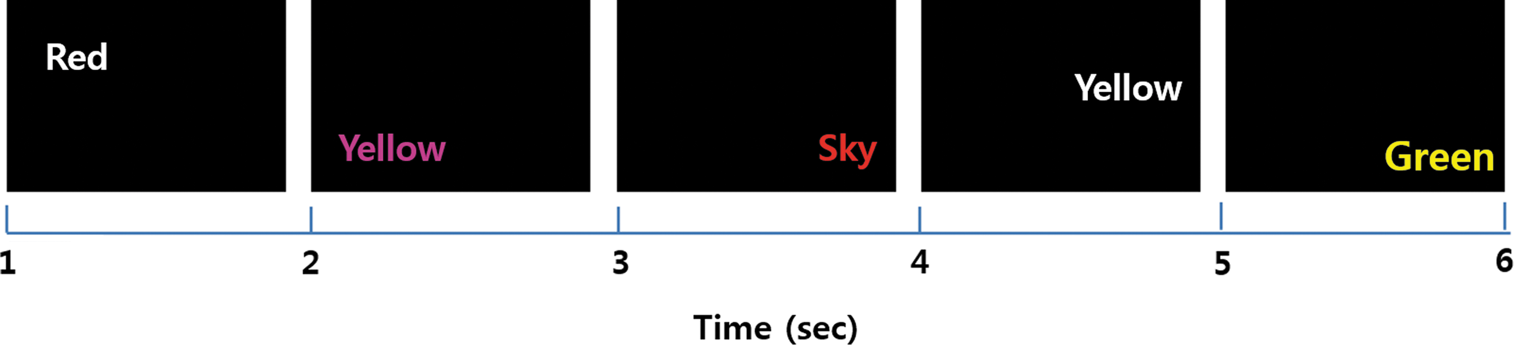
Example of the sequential visual stimuli of CWT across time. CWT, color word test.

Fig. 3.

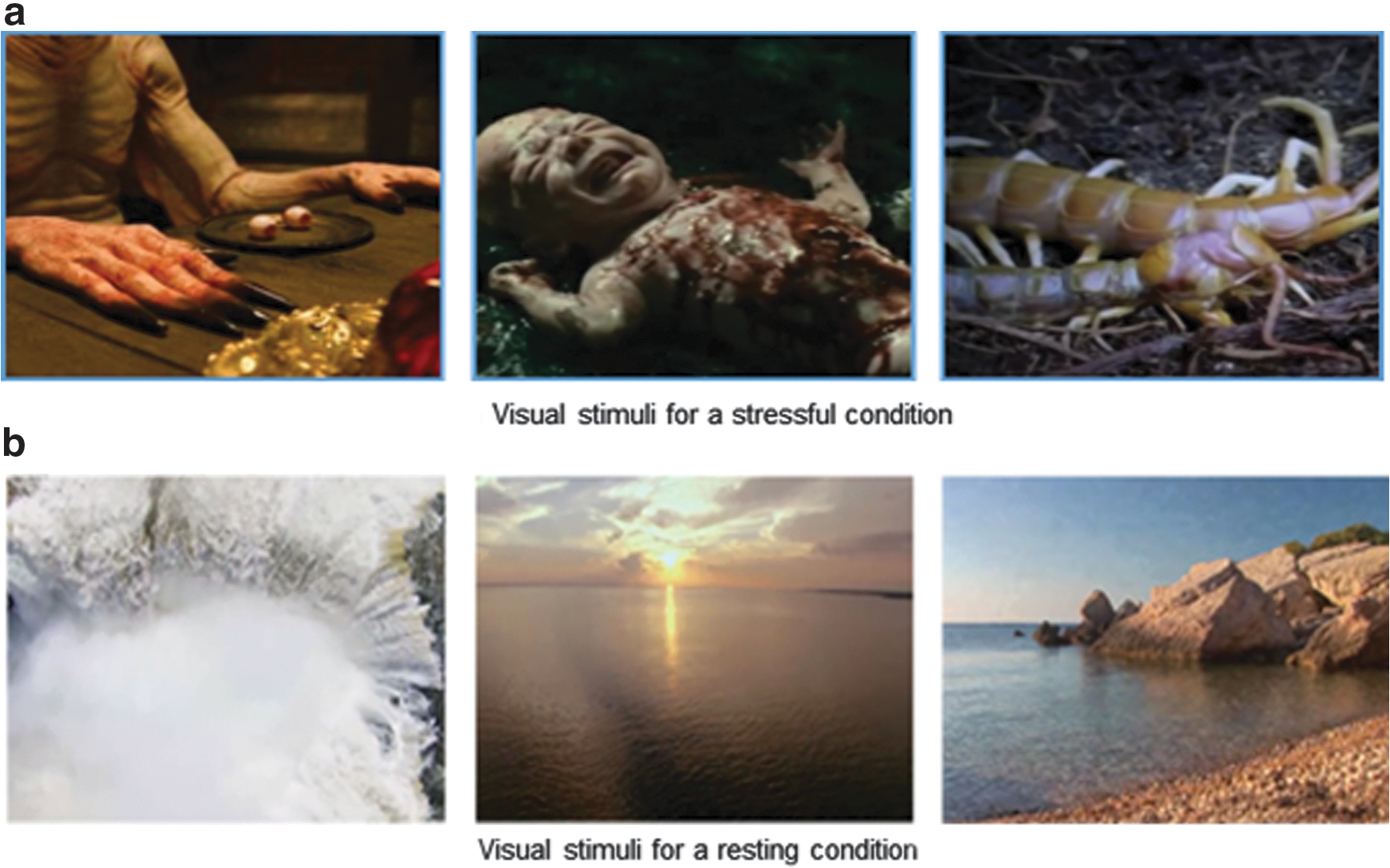
Examples of the visual stimuli to elicit. (a) Visual stimuli for a stressful condition. (b) Visual stimuli for a resting condition.

Table 1.

Procedure of the Stressor Tests

TRIALS	DURATION (MIN.)
Rest session	4
Arithmetic	5
Rest session	4
CWT	5
Rest session	4
Interview	5 (+5 for preparation)
Rest session	4
Visual stimuli	5
Rest session	4
Cold pressor	1
Rest session	4

CWT, color word test.

The details of the stressful experimental protocols are described in Table 2.

Table 2.

Experimental Protocol Descriptions for Case1

PROTOCOLS	DESCRIPTIONS
Arithmetic	Subtract 13 from 1,022 without writing, in which subjects start over when a wrong answer is given.
CWT	On a screen, colored words are shown, and subjects are instructed to say the color of the letters, not the color that the word represents (Fig. 2).
Interview	Subjects prepare an answer to the interview questions for five minutes, and then perform an interview for an additional five minutes.
Visual stimuli	Five video streams are shown to subjects, which trigger a stressful condition (Fig. 3).
Cold pressor	Subjects are instructed to keep their hand in cold water (0°C–4°C) for a minute.

This study was reviewed and approved by the Institutional Review Board at the Korea National Institute for Bioethics.

Case 2- KU Leuven university mental arithmetic task experiments

Thirty healthy subjects were recruited at Maastricht University (27 female; 3 male) using flyers and posters. Inclusion criteria were (a) age 18–35, (b) sufficient command of the Dutch language to understand and give informed consent, and (c) mental competence to understand and follow instructions. Participants were excluded if they previously participated in a study using a mental arithmetic task. In a subsample of nine participants, heart rate was measured during the experimental task using three chest leads like Figure 1b, where sampling frequency was 1000 Hz.

During the experiment, psychosocial stress was induced with a modified version of the Montrèal Imaging Stress Test (MIST), a mental arithmetic task with a psychosocial evaluation component in the form of scripted negative feedback by an experimenter (Pruessner JC, Champagne F, Meaney MJ, Dagher A, 2004). The task consisted of four runs, each divided in six 7-min blocks (30 s rest; 60 s control; 120 s experimental; 30 s rest; 60 s control; 120 s experimental). During the experimental blocks, participants solved mathematical equations under time pressure on a computer, while their performance was visualized as an arrow on a performance bar. The task difficulty was manipulated by a computer algorithm such that participants on average were able to provide the correct answers in time only for 60–70% of the cases. In the current version, participants were always tested in couples, sitting in separate testing rooms. A social defeat component was added by a cover story saying that participants were competing against each other and an arrow indicating the opponent's performance was visible above the performance of the participant. In reality, the opponent's arrow was manipulated by the program to always outperform the participant's and both participants were made to believe that their opponent performed better. During the control blocks, participants solved equations without time limit and performance arrows; the rest blocks existed of passive watching of the task interface.

As basic preprocessing, a 2000-order FIR notch filter was applied to remove the power line noise in the frequency range 48–52 Hz, and an additional 3000-order FIR bandpass filter was applied to keep the frequency components in the range 1.5–150 Hz.

This study was approved by the Ethics Committee Psychology of the Maastricht University. Participants were treated in accordance with American Psychological Association standards. All participants gave written informed consent before the study.

Conventional ECG analysis methods

Conventional ECG features were extracted by the methods shown in Table 3, based on the predefined formulas.¹¹ In addition, long time series of ECG signal, 5 min long, were utilized for the standard HRV parameter analysis, impractical in real-time stress classification.

Table 3.

The Correlation Coefficients Between Short 10-S HRV Parameters and Standard 5-Min HRV Parameters and Their Descriptions⁷

HRV PARAMETERS	CORRELATION COEFFICIENTS	DESCRIPTIONS OF HRV PARAMETERS
HR	0.9321 ^a	Mean average NN intervals
SDNN	0.6203	Standard deviation of NN intervals
RMSSD	0.636	Square root of the mean average of the sum of the square
pNN50	0.6528	Percentage of absolute difference in successive NN values >50 (ms)
LF	0.4156	LF (low frequency), power of range 0.04–0.15 Hz
HF	0.6294	HF (high frequency), power of range 0.15–0.4 Hz
TF	0.5397	TF (total frequency), power of range 0.14–0.4 Hz of the PSD of NN intervals
VLF	0.0357	VLF (very low frequency), power of range 0–0.04 Hz
nLF	0.3869	Proportion of LF to LF+HF of range 0.04–0.4 Hz
nHF	0.3869	Proportion of HF to LF+HF of range 0.04–0.4 Hz
LF/HF	0.1503	Proportion of LF to HF

Kruskal–Wallis test: p > 0.5.

The underscored parameters represent the highly correlated HRV parameters compared to the conventional 5 m HRV parametes (correlation coefficient > 0.6).

HRV, heart rate variability; NN, normal to normal.

To compare with the performance of the proposed deep learning approach, this conventional HRV analysis was conducted as a benchmark method. For HRV experiments, two experimental cases were tested according to the correlation coefficients between standard HRV parameters and 10-s HRV parameters.⁷

The first HRV experiment was a classification experiment using only one parameter (heart rate, the correlation coefficient, >0.9, HRV-1 case), and the second experiment was a classification experiment with four parameters (the correlation coefficient >0.6, HRV-4 case). For HRV-4 case, HR, SDNN, RMSSD, pNN50, and HF parameters satisfied the conditions shown in Table 3.⁷ However, pNN50 was excluded because of abnormal extracted values. Therefore the four parameters underscored in Table 3 (HR, SDNN, RMSSD, and HF) are used as main features, except pNN50 for HRV-4 case.

The spectrogram of ECG signals was also used as a benchmark method. Although frequency analysis has been a popular method to look into the physiological signal, it is also based on predefined basis functions such as sinusoids during the process of Fourier transform. In addition, the physiological signal-like ECG is nonlinear and nonstationary, hard to be generalized with a fixed basis function and deterministic/stationary model.¹²

This study proposes an end-to-end deep learning method to overcome these drawbacks by extracting the features from the input data itself without an unrealistic predefined basis function or model. To evaluate the performance of the proposed approach, the performance of HRV parameters with conventional classifiers was tested (Fig. 4a). In addition, the spectrogram/frequency analysis was also conducted to compare the proposed method with the Fourier-based linear/deterministic analysis. In this spectrogram analysis, the transformed frequency amplitude value using Fourier transform was used as a feature to classifiers, depicted in Figure 4b.

Fig. 4.

Conventional ECG analysis methods. (a) HRV parameter analysis. (b) Spectrogram analysis. HRV, heart rate variability.

The initial setup of the deep learning architecture

As mentioned earlier, most of the conventional data analytics for the stress monitoring using physiological signals required prior knowledge-based feature extraction. The main purpose of this study is to extract hidden feature representations using 1D CNNs by training the whole process from raw signal input to class label outputs in the manner of seamless end-to-end learning.^8,9,13

CNNs, one of the popular deep learning models, were used as a basic unit in the whole learning architecture. CNN models have shown outstanding performance in the field of computer vision, which was developed for processing vision information based on the human optic nerve structure.^8,9 CNNs have two main layers, a convolution layer and a pooling layer, which have the advantage of reducing overall model complexity because the main characteristics of CNNs are sparse weight and parameter sharing.

In this study, a 1D CNN was used to generate the hidden representations of a univariate time series ECG signal. The operation procedure and details of the convolution layer are illustrated in Figure 5a, where the 1D filter is implemented in each channel of the hidden layer. During the learning process of CNNs, the filter coefficients are determined with an optimization learning process using error back propagation according to input signals and output labels.

Fig. 5.

1D Convolution and pooling operations. (a) 1D convolution operation. (b) 1D pooling operation.

Figure 5b illustrates the structure of the pooling layer after the convolution operation. Since the convolution operation produces similar outputs across time, subsampling by taking the maximum or average value in a particular window size makes it possible to reduce the feature dimension. In addition, the patterns of data could be well recognized owing to this subsampling, choosing only one value within the pooling operation window, despite data variations such as placement, scale, and rotation of data.^14,15

In the early stage of this study, the initial setup of the deep learning model was designed by deeply stacking the convolution and pooling operations in three layers (Fig. 6). In this model, three layers of CNNs were built with 50, 30, and 10 channel outputs, respectively. The convolution filter length of the first CNN layer was set as 500 points (0.5-s) to cover the particular shapes of ECG signal empirically. This structure and its parameters were decided and tuned empirically based on the previous studies on designing deep learning models.^16
–18

Fig. 6.

Initial setup empirical deep learning architecture

In addition, batch normalization and dropout layers were included to prevent overfitting, resulting in improved performance. The batch normalization was performed in mini batch units, known to prevent exploding/vanishing of parameters when gradient descent is used.¹⁹ Dropout is a regularization technique to prevent the overfitting problem of the neural network on training data. The term “dropout” refers to dropping out units (both hidden and visible) in the neural network, by which the learning is performed in the form of randomly switching off a certain node. In other words, it has the effect of implementing multiple structures of the neural networks, which can yield performance with their ensemble learning.²⁰ The loss function was the categorical cross entropy and the Adadelta algorithm was used as its optimizer. All learning parameters used the default setting according to the literature (learning-rate = 1.0, decay = 0.0).²¹

After the CNN layers, the fully connected structure such as Multilayer Perceptrons (MLP) was used to derive the final output labels.

After the initial setup of the deep learning model with heuristically defined parameters, its performance was compared with those of the conventional HRV & spectrogram methods. In this benchmark test, the model outperformed the conventional methods as can be seen in Table 4.

Table 4.

The Performance Comparison Between the Initial Setup Empirical Deep Learning Model and Conventional Methods (HRV-1, HRV-4, and Spectrogram)

ACCURACY	HRV-1	HRV-4	SPECTROGRAM	INITIAL SETUP EMPIRICAL DEEP LEARNING MODEL
Case 1	0.6796	0.7105	0.6669	0.7933
Case 2	0.5676	0.6307	0.6069	0.6625

The deep ECGNet

Although the initial setup of the deep model with empirically defined parameters had already outperformed the conventional method, a systemic approach to optimize the parameters while considering the fundamentals of the CNNs algorithm was crucial to maximize the performance of our proposed model.

In our empirical deep learning model, phases of ECG peaks according to a partial segment of ECG signal, was not considered in depth. However, to improve the performance to classify the stressful conditions, the phase of ECG peak should be considered because the referenced ground line is needed to capture the differences of ECG signal characteristics.

Peak detection and alignment algorithms to adjust peaks of signals need an additional preprocessing procedure. However, performing this preprocessing process does not fit the basic idea of deep learning that a feature can be generated by itself to recognize a pattern.

CNNs are known to be the most powerful algorithm in the image recognition area, and have an especially clear and strong advantage to deal with variances of data such as variations in the location of images. For example, in the Mixed National Institute of Standards and Technology handwritten digits recognition problem, CNNs was able to recognize the digits with only a few errors even though placement, scale, and rotation of the digits were changed.²² This was due to the pooling operation, able to extract specific area features by subsampling.^14,15 Inspired by this characteristic of the pooling operation, it was applied to 1D ECG signals.

For 1D time series signal data, the subsampling of the pooling operation with a specific duration is able to overcome the peak phase difference problems, because the features of a signal are inevitably extracted in a given pooling window regardless of the peak point.

Therefore, the model could capture the one cycle feature of a signal without considering any preprocessing if the pooling length was set as one cycle of the ECG signal. As can be seen in Figure 7, six figures display typical ECG patterns of randomly picked 3 ECG signals from the dataset, including P, Q, R, S, and T waves in various length windows. In the figures, only the 0.8-s window case (Fig. 7e) could contain one whole shape of the three signals within a one-segment window. In this figure, the 0.8-s window was matched with the average heart beat duration (0.7849 s) calculated using the ECG dataset from Table 5.

Fig. 7.

Raw ECG signal plots corresponding to segment time windows. (a) 0.1 s window(100-point), (b) 0.2 s window(200-point), (c) 0.4 s window(400-point), (d) 0.5 s window(500-point), (e) 0.8 s window(800-point), and (f) 1.6 s window(1600-point).

Table 5.

Average Heart Rates (Heart Beat Duration)

HEART RATE (SEC, MEAN/STD)	STRESS	RESTING	AVERAGE	TOTAL AVERAGE
Case 1	0.8095/0.1085	0.7944/0.1121	0.8028/0.1104	0.7849/0.1271
Case 2	0.7640/0.1420	0.7467/0.1492	0.7555/0.1458

Based on this, we also assumed that the one-cycle filter length of convolution operation would be effective for the same reason as with the pooling operation. The convolution and pooling operations were set to a one-cycle filter length and pooling length, respectively, which made the CNNs able to capture the ECG characteristics with the whole complete shape information of the signal.

To verify this assumption, various experiments were conducted corresponding to the various convolution filters and pooling lengths. These experimental results are shown in the result section.

Although a CNNs architecture usually uses a fully connected layer to the output,^8,9 an RNN structure with long short-term memory was adopted for the proposed model considering the sequential patterns of the ECG time series. To use an RNN model in the final layer, it is necessary to preserve the sequential time order of the CNNs output representation of the ECG signals.

As shown in Figure 8, the proposed simple model architecture based on the hypothesis was designed to compare it with the initial setup of the deep learning model. This control model has only one CNN stage, which could produce the feature representation with a one-cycle filter length and pooling length, and also has two RNN layers to generate feature vectors using sequential features extracted by CNN stage.

Fig. 8.

The proposed optimal RCNN deep learning architecture: Deep ECGNet. RCNN, recurrent and convolutional neural networks.

To analyze the performance of the entire deep learning architecture, additional comparative architecture models were also constructed in Figure 9.

Fig. 9.

The various deep learning architectures. (a) Intial setup empirical model, (b) General CNNs model, (c) Proposed Deep ECGNet model. CNN, Convolutional Neural Network.

Figure 9a is the initial setup of the deep learning model with RNN layers instead of fully connected layers, Figure 9b is the general deep CNN's model version of the Deep ECGNet, which has the fully connected layers instead of RNN layers, and Figure 9c is the proposed reference control model. The proposed model is denoted as “Deep ECGNet.”

As can be seen in Table 6, the Deep ECGNet requires less hardware resource and has a faster execution time than those of the initial setup of the deep learning model.

Table 6.

The Usage of Resources and Runtimes According to Model Structures

STRUCTURE	3CONVLAYER500PLEN 2RNN^*	3CONVLAYER800PLEN 2RNN^*	1CONVLAYER800PLEN 2FULLYCONNECTED^†	1CONVLAYER800PLEN 2RNN: THE DEEP ECGNET^‡
# of parameters	49,092	49,092	43,724	39,772
Memory usage (byte)	4,752,992	4,550,400	3,802,856	3,805,096
Runtime(sec): Case1	19,782	19,604	16,733	17,714
Runtime(sec): Case2	13,674	13,442	11,291	12,115

See figure 9a.

†

See figure 9b.

‡

See figure 9c.

For each model, comparative experiments, in terms of accuracy, were conducted on both Case 1 and Case 2.

All experiments of our studies were conducted with a five-fold crossvalidation method with 60% training, 20% validation, and 20% test sets, and on a 3.30 GHz Intel Core i5 processor with 64GB of RAM and two NVIDIA TiTAN Xp GPU with Ubuntu Linux v14.04.5. In addition, the scikit-learn v0.18.1 library and the KERAS v2.0.2 were used for conventional classification and deep learning algorithms, respectively.

Results

The main purpose of this study is to classify the stressful and resting states corresponding to the ECG responses to stress eliciting stimuli. This binary classification problem was analyzed using the proposed deep learning methods and conventional methods as benchmark tests.

To evaluate the performance using conventional features, 10 conventional machine learning algorithms were used as classifiers. As shown in Table 7, HRV-1 and HRV-4 yielded an average classification accuracy of 67.96% and 71.05% for Case 1, and of 56.76% and 63.07% for Case 2. The highest classification result for Case 1, 72.90% with HRV-4, was obtained using the Random Forest algorithm, and the highest classification result for Case 2 was 66.64% using the MLP algorithm. As shown in Table 8, the average accuracies using spectrogram features were 58.71% for Case 1 and 54.83% for Case 2, respectively. The maximum accuracy for Case 1, 66.69%, was obtained using the Random Forest algorithm and the maximum accuracy for Case 2 was 60.69% using the Naive Bayes algorithm. In Table 7 and Table 8, the underscored values represent the best performance algorithm for each case.

Table 7.

Conventional Method Results Accuracies–HRV Parameters

	CASE1		CASE2
ALGORITHMS	HRV-1	HRV-4	HRV-1	HRV-4
Nearest neighbors	0.6807	0.7108	0.5646	0.6389
Linear SVM	0.6801	0.6937	0.5660	0.6505
RBF SVM	0.6949	0.7239	0.5583	0.6225
Gaussian process	0.6920	0.7261	0.5597	0.6447
Decision tree	0.6591	0.6875	0.5590	0.6082
Random forest	0.6710	0.7290	0.5708	0.6220
MLP	0.6813	0.7188	0.5757	0.6664
AdaBoost	0.6528	0.6994	0.5715	0.5730
Naive Bayes	0.6926	0.7023	0.5743	0.6288
QDA	0.6915	0.7131	0.5757	0.6521
Average accuracy	0.6796	0.7105	0.5676	0.6307
STD	0.0146	0.0143	0.0069	0.0266

Underscored values represent the best performance algorithm for each case.

Table 8.

Conventional Method Results Accuracies–Spectrogram

ALGORITHMS	CASE 1	CASE 2
Nearest neighbors	0.6259	0.5913
Linear SVM	0.5484	0.57
RBF SVM	0.5484	0.5
Gaussian process	0.5559	0.5
Decision tree	0.5934	0.5344
Random forest	0.6669	0.5363
MLP	0.5484	0.5619
AdaBoost	0.6298	0.5587
Naive bayes	0.6091	0.6069
QDA	0.5448	0.5231
Average accuracy	0.5871	0.5483
STD	0.0441	0.0360

Underscored values represent the best performance algorithm for each case.

Based on the hypothesis, the deep learning architecture experiments were conducted with the assumed optimal convolution filter and pooling size. (Where, the “fLen” means convolution filter length, and “pLen” means pooling operator length.)

In Figure 10, the first 2 results (500fLen3convLayer500pLen and 500fLen3convLayer800pLen) are the initial setups of the deep learning network with different pooling lengths (Fig. 9a). The third result (500fLen800pLen _MLP) is the model having two fully connected layers instead of RNN layers (Fig. 9b). The final result is the proposed Deep ECGNet (Fig. 9c). As can be seen in Figure 10, our proposed Deep ECGNet model (Fig. 9c) showed the best results (85.77% and 73.12%), better than those of the other deep learning architectures.

Fig. 10.

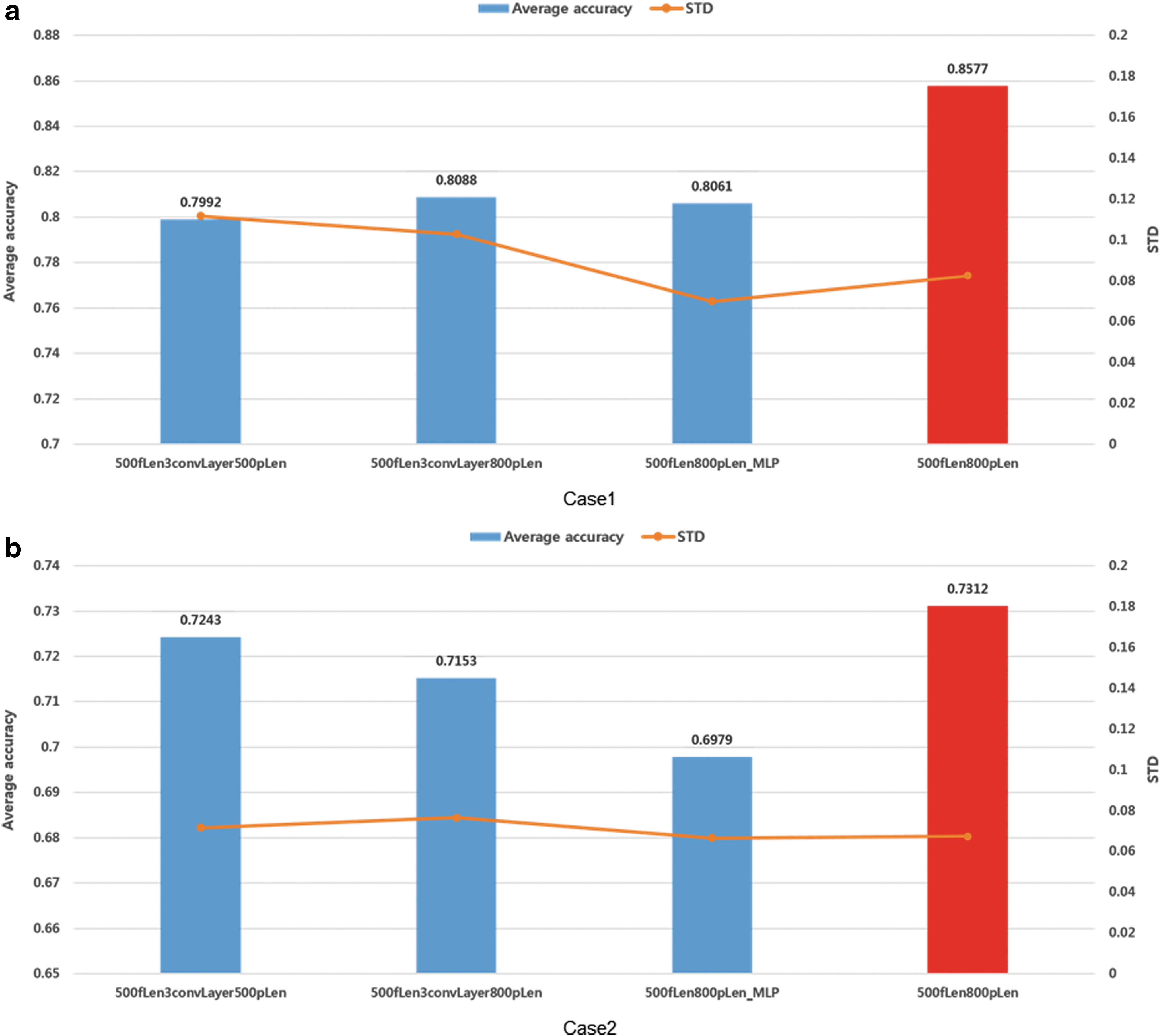
The experimental results corresponding to various deep learning architectures. (a) Case 1 (b) Case 2.

To reduce dimensions of data, a stride size adjustment can be considered in the CNNs algorithm as well as the pooling operation. The stride size in CNNs is the step size of convolution operation from the current to the next convolution operation. Default setting is a unit stride that the convolution operation of every sliding moves in one data point. Therefore, for example, if the stride size is set to 10, it will give the 1/10 sampling effect to data. For reducing the training time, this experiment was conducted because the convolution operation was a dominant factor for running time of the training process. Figure 11 shows the experimental results of this.

Fig. 11.

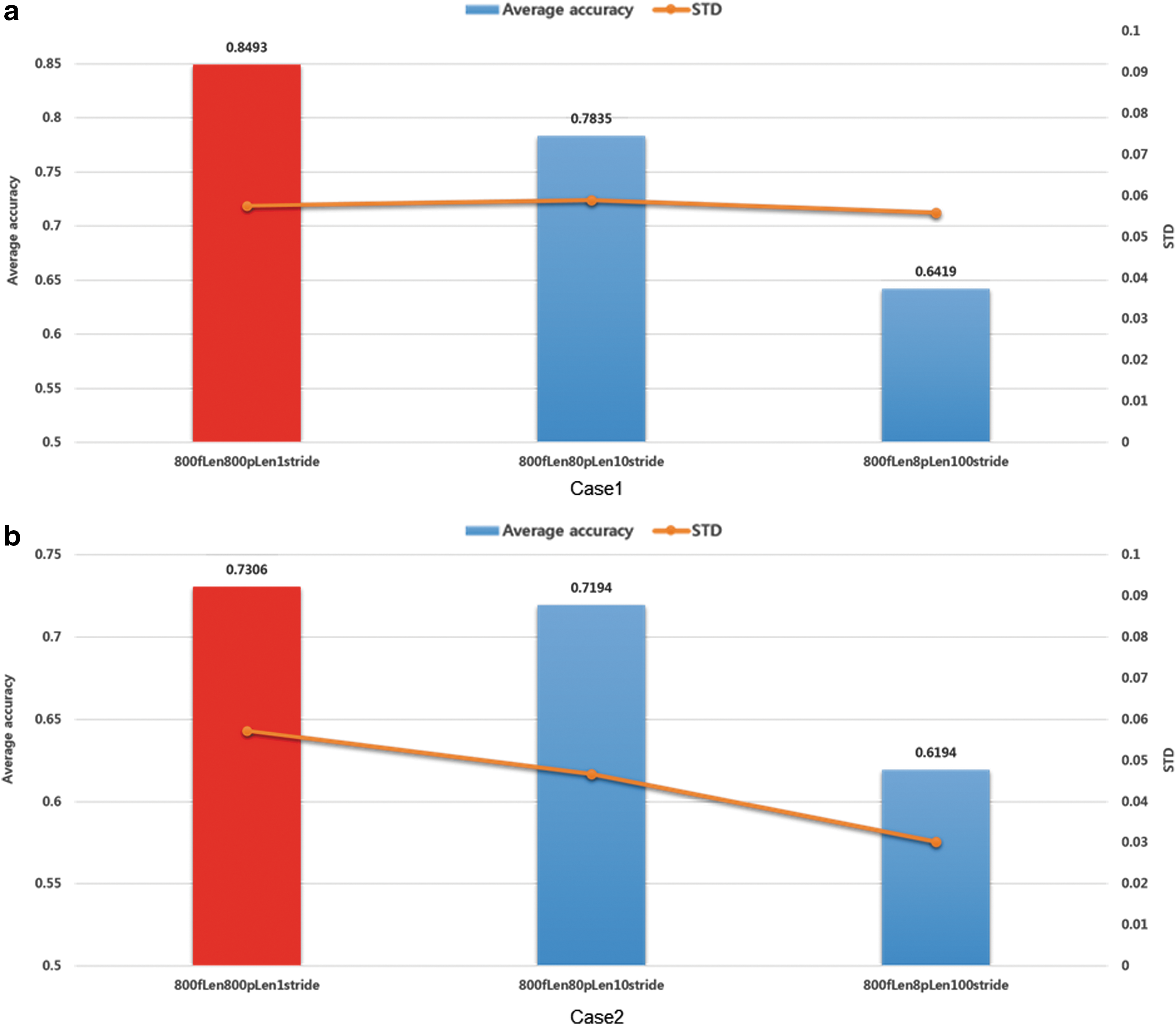
The experimental results corresponding to stride sizes. (a) Case 1 (b) Case 2.

Experimental setups for three cases were made to yield the same sequence feature length after the convolution layers as the same as that of the previous 800-point pooling case. In Figure 11, the first one “800fLen800pLen1stride” was the original model, and the second one “800fLen80pLen10stride” was that having 10-stride and 80-point pooling. The final one “800fLen 8pLen100stride” was that having 100-stride and 8-point pooling. All these three models generated the same-length sequence data after the CNNs stage.

However, as you can see in Figure 11, as the stride size was increased, the accuracy was decreased. This result infers that the amount of information is decreased as stride is increased. In other words, if the stride size is set to 10, the number of features after the convolution operation will be reduced 1/10 compared with that of the unit stride case. Therefore, if the hardware resource and time for training are enough, the unit stride size would be recommendable based on these results. However, longer stride size could be applied in the initial setup of the structural optimization process, because the running time is faster than that of a unit stride case because of the reduced multiplication operations of convolution operation as shown in Table 9.

Table 9.

Runtime Comparison Results According to Stride Sizes

RUNTIME (SEC)	UNIT STRIDE	10-STRIDE	100-STRIDE
Case 1	17,714	11,348	8,597
Case 2	11,136	6,140	5,197

From the constructed optimal recurrent and convolutional neural networks (RCNN) architecture based on the hypothesis about one cycle length for convolution filter length and pooling length and the results in Figure 10, several experiments were also conducted to find the optimal parameters. First of all, optimal pooling length experiments were conducted with fixed convolution filter length. As you can see in the Figures 12 and 13, each fixed convolution filter length was 500-point and 800-point, respectively, because the convolution filter length of the first initial setup of the deep learning model was 500-point, and one-cycle length of ECG signal was 800-point corresponding to Table 5 (average heart beat duration: 0.7849 s, 800-point in 1000 Hz sampling rate). As you can see in the graphs, experimental results showed the best classification accuracies when pooling length was set to 800-point. The only “800fLen400pLen” of Figure 13a Case 1 showed slightly better performance than that of “800fLen800pLen”, but the difference was negligible. Based on these results, the established hypothesis that the optimal pooling operation length was one cycle of ECG signal could be accepted.

Fig. 12.

The pooling length experimental results corresponding to various pooling sizes with fixed 500-point convolution filter length. (For example, where “800conv800pooling” means 800-point convolution filter length and 800-point pooling length.) (a) Case 1 (b) Case 2.

Fig. 13.

The pooling length experimental results corresponding to various pooling sizes with fixed convolution filter length(800-point). (a) Case 1 (b) Case 2.

Similar to the pooling length experiments, convolution filter length experiments were also conducted. For this experiment, the optimal fixed 800-point pooling length based on the results in Figures 12 and 13 were set for all optimal convolution filter experiments. At the beginning of the experiment, the filter lengths were set to 100, 200, 400, 800, and 1600 points in the same manner as the pooling length experiment. However, as you can see in Figure 14, both Case 1 and Case 2 showed the best performances (86.37% and 73.06%) when 400-point and 800-point convolution filters were applied, respectively. So, we added an experiment of 600-point filter length between 400-point and 800-point, and finally, both cases showed the best performances (87.39% and 73.96%) with the 600-point convolution filter.

Fig. 14.

The convolution filter length experimental results corresponding to various convolution filter sizes with fixed pooling length (800-point). (a) Case 1 (b) Case 2.

The reason why it was showing the best result at 600-point is analyzed as follows.

The ECG signal has inherent waveform characteristics shown in Figure 15. Therefore, it is very important to analyze the characteristics of all these P, Q, R, S, and T waveforms.²³ From the inherent characteristics of these ECG P, Q, R, S, and T waveforms, we were able to find out why the 600-point convolution operation showed the best performance. To perform the 800-point pooling operation, the convolution operation must be performed 800 times, moving the convolution filter. Figure 16 shows the data region (purple box) covered by the filter from the start position to the end position of convolution operation according to the convolution filter lengths. For the 400-point filter, there is no interference with the next signal as shown in Figure 16c, but it cannot cover the entire P, Q, R, S, and T (in this case, T-wave) of the ECG signal as shown in Figure 16b. For the 800-point filter, it covers the entire P, Q, R, S, and T regions as shown in Figure 16h. However, there is a large interference with the next signal as shown in Figure 16i. The 600-point filter shows the best performance in Figure 14, the entire P, Q, R, S, and T regions are covered as shown in Figure 16e, and there is a less interference with the next signal as shown in Figure 16f. Therefore, the 600-point convolution filter length was the optimal filter length, and moreover, we were able to find out that this 600-point (0.6 s) filter length was consistent with the normal PQRST ECG wave patterns duration (PR interval + QT duration = 0.57–0.67 s: 570–670 points in 1 KHz sampling rate) from the Figure 15.

Fig. 15.

The ECG curve with its most common waveforms. Important intervals and points of measurement are depicted. ECG interpretation requires knowledge of these waves and intervals.²¹

Fig. 16.

The coverages of convolution operation within ECG heart beat duration (0.8 s) with 0.4 s (a–c), 0.6 s (d–f), 0.8 s (g–i) width convolution filters, respectively. (Where, the red line is the starting point of ECG P-wave, and the purple box is the coverage region of convolution filter). (a) Start position with 400 filter. (b) PQRST position with 400 filter. (c) End position with 400 filter. (d) Start position with 600 filter. (e) PQRST position with 600 filter. (f) End position with 600 filter. (g) Start position with 800 filter. (h) PQRST position with 800 filter. (i) End position with 800 filter. PQRST, ECG wave patterns.

In addition to the results in Figure 16, you can see that the proposed setup of parameters is able to capture the PQRST waveforms with minimum interference in the convolution operation region when 800-pooling is applied regardless of the segment window positions as shown in Figure 17.

Fig. 17.

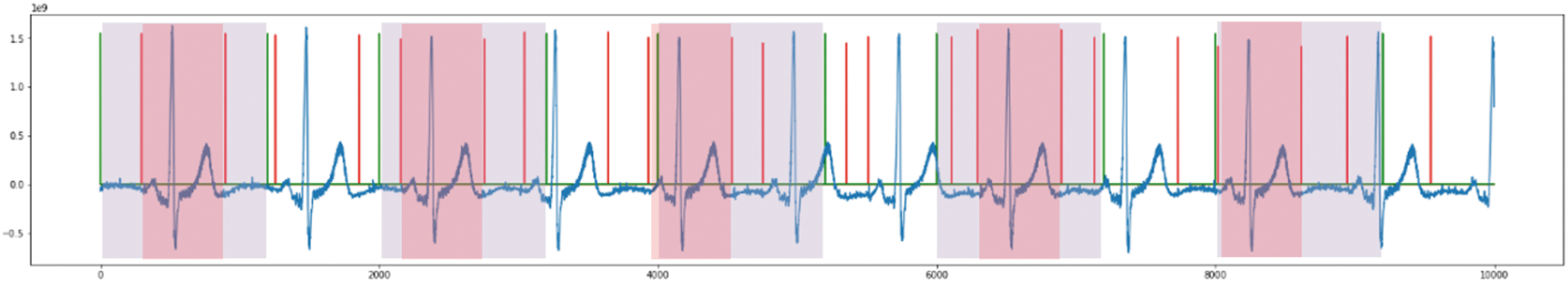
The captured PQRST waveforms in the convolution operation region with 800-pooling (Where, the red box is the PQRST regions of ECG signal and the purple box is the convolution operation region when 800-pooling is applied).

As a result, the specific combination of convolution filter (0.6 s) and pooling (0.8 s) lengths is able to extract characteristics of one ECG waveform regardless of the signal segment window position without any feature engineering methods.

To validate whether the trained convolution layer generates specific feature patterns, we visualized the representation of the hidden layer after convolution and the activation function layer (ReLU) as shown in Figure 18. For the Deep ECGNet, the convolution layer output was set to generate 50 channel feature maps and we could see specific spiky patterns around the starting point of the original ECG P wave (red line) in several channels as shown in Figure 18b–g. This result means that the trained convolution filter worked properly as a kind of masking filter for the P, Q, R, S, and T waveforms of ECG signals.

Fig. 18.

Visualizations for the hidden layer representation examples after convolution & activation function layer (ReLU) (Where, the red line is the starting point of ECG P-wave). (a) The original ECG signal. (b) Hidden representation feature map of Ch.3. (c) Hidden representation feature map of Ch.5. (d) Hidden representation feature map of Ch.13. (e) Hidden representation feature map of Ch.23. (f) Hidden representation feature map of Ch.36. (g) Hidden representation feature map of Ch.43.

Lastly, as shown in Figure 19, it was confirmed that the proposed deep learning framework showed the highest stress determination performance compared with the conventional stress analysis methods. For the proposed optimal RCNN deep learning model, the result showed the highest accuracy of 87.39% for Case 1 and 73.96% for Case 2, respectively. These results indicate the performance improvements of 16.22% for Case 1 and 10.98% for Case 2, respectively, as compared with the HRV-4 method.

Fig. 19.

The final experimental results compared with conventional ECG analysis methods. (a) Case 1 (b) Case 2.

Figure 20 shows the procedure of the feature extraction sequence of the Deep ECGNet. As you can see on the plot in Figure 20, specific overlapping different patterns are observed after the final RNNs stage corresponding to the stress (top left plot) and resting states (top right plot), respectively.

Fig. 20.

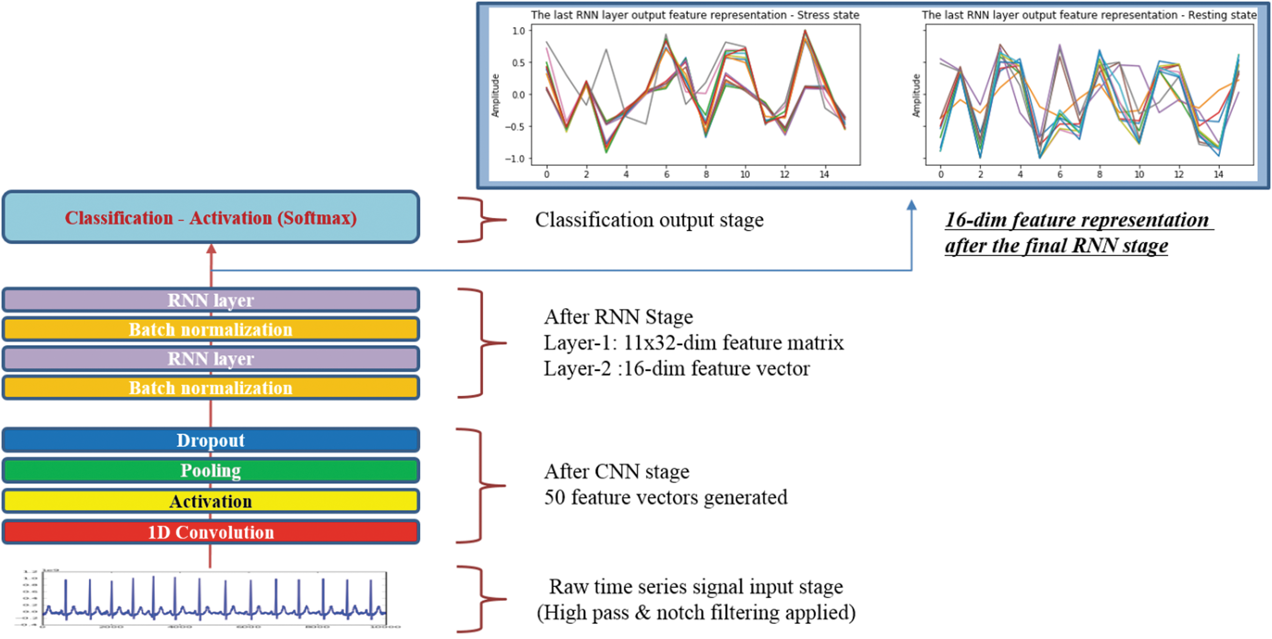
The procedure of the proposed system to generate optimal features.

Discussion & Conclusion

This study proposes an optimal deep learning framework to analyze ECG signals for monitoring mental stress of humans without conventional feature engineering. Another aspect is the theoretical study on how to design the deep learning structure for data with periodicity.

The experimental results demonstrated that the proposed method produced superior performance compared with the conventional methods. In particular, there have been a few number of significant HRV parameters for an ultra short-term 10-s ECG signal according to⁷ the method of using HRV parameters that could only use limited information to estimate the mental stress. In addition, the 10-s short-time window could not provide enough resolution in frequency, lacking sufficient spectral information from the spectrogram features.

On the other hand, the proposed deep learning model could successfully extract the basic characteristics of ECG signals for the determination of the stress conditions through 1-D CNN & RNN stages. Its whole training process could determine proper filter coefficients like a masking filter to extract important features of ECG signals.

Through the various experiments, we proposed the optimal deep learning framework for stress recognition with the optimal convolution filter length and pooling length. The key point is that the proposed model is able to extract key features of the exact one-cycle ECG signal based on the specific durations. This process is a typical designing process of a deep learning model using prior knowledge of data.

Moreover, RNNs were added to extract the final feature using the extracted sequential features from the CNNs' stage. In the RNNs' representation, consistent overlapping patterns across trials could be noticed, that is, the RNNs at the end stage worked properly as a pattern decoder (Fig. 20).

Based on the results, the structure of the network model could be more compact and concise than that of the initial setup of the deeper network. The number of parameters and memory usage were also reduced compared with those of the initial setup of the deeper model. Additionally, the proposed model showed even better performance than that of the previous various methods. This means that a very deep structure is not necessary if we know prior knowledge of given data and could apply it to the model in the aspects of performance and hardware resources.

This study could be applicable to other time series signals with periodicity.

For future works, a multimodal physiological signal deep learning framework for human emotion recognition will be studied using the results from this study.

Footnotes

Acknowledgments

This work was partly supported by Samsung Electronics Semiconductor Division, a National Research Foundation of Korea (NRF) grant funded by the Korea government (MSIP) (No. NRF-2017R1A5A1015596), the Institute for Information & Communications Technology Promotion (R0126-16-1072-SW.StarLab), and a 2017 Research Grant from Kwangwoon University.

Disclosure Statement

No competing financial interests exist.

References

Kreibig

. Automatic nervous system activity in emotion: A review. Biol Psychol, 2010; 84:394–421.

Hjortskov

, Rissén

, Blangsted

, Fallentin

, Lundberg

, Søgaard

. The effect of mental stress on heart rate variability and blood pressure during computer work. Eur J Appl Physiol, 2004; 92:84–89.

Belkic

, Landsbergis

, Peter

, Schnall

, Baker

, Theorell

, Siegrist

, Karasek

. Research findings linking workplace factors for CVD outcomes: Psychosocial factors—review of the empirical data among men. Occup Med, 2000; 15:24–46.

Karthikeyan

, Murugappan

, Yaacob

. Detection of human stress using short-term ECG and HRV signals. J Mech Med Biol, 2013; 13:1350038-1-29.

Task Force of the European Society of Cardiology and the North American Society of Pacing and Electrophysiology. Heart Rate Variability: Standards of measurement, physiological interpretation, and clinical use. Eur Heart J, 1996; 7:1043–1065.

Holly

, Alison

, Carlo

, Egbert

, Carl

, Barbara

, Michele

, Gregg

, Antoine

, Jaime

. Impact of acute mental stress on sympathetic nerve activity and regional blood flow in advanced heart failure. Circulation, 1997; 96:1835–1842.

Baek

, Cho

, Woo

. Reliability of ultra short-term analysis as a surrogate of standard 5-minute analysis of heart rate variability. Telemed J E Health, 2015; 21:404–415.

LeCun

, Bengio

, Hinton

. Deep learning. Nature, 2015; 521:436–444.

LeCun

, Kavukcuoglu

, Farabet

. Convolutional networks and applications in vision. Circuits and Systems (ISCAS), Proceedings of 2010 IEEE International Symposium on. Paris, France: IEEE, 2010.

10.

Lipton

, Berkowitz

, Elkan

. A critical review of recurrent neural networks for sequence learning. arXiv Preprint arXiv, 2015:1506.00019.

11.

Taelman

, Vandeput

, Spaepen

, Van Huffel

. Influence of mental stress on heart rate and heart rate variability. In 4th European Conference of the International Federation for Medical and Biological Engineering. Berlin, Heidelberg: Springer, 2009:1366–1369.

12.

Park

, Plank

, Snider

, Kim

, Huang

, Gepshtein

, Poizner

. EEG gamma band oscillations differentiate the planning of spatially directed movements of the arm versus eye: Multivariate empirical mode decomposition analysis. IEEE Trans Neural Syst Rehabil Eng, 2014; 22:1083–1096.

13.

Shi

, Bai

, Yao

. An end-to-end trainable neural network for image-based sequence recognition and its application to scene text recognition. IEEE Trans Pattern Anal Machine Intell, 2016:39:2298–2304.

14.

LeCun

. Learning invariant feature hierarchies. In Computer Vision–ECCV 2012. Workshops and Demonstrations. Berlin/Heidelberg: Springer, 2012.

15.

LeNet-5, convolutional neural networks. Available at: http://yann.lecun.com/exdb/lenet (last accessed September 15, 2017 ).

16.

Cui

, Chen

. Multi-scale convolutional neural networks for time series classification. arXiv Preprint arXiv, 2016:1603.06995.

17.

Yang

, Nguyen

, San

, Li

, Krishnaswamy

. Deep convolutional neural networks on multichannel time series for human activity recognition. Buenos Aires, Argentina: IJCAI, 2015:3995–4001.

18.

Ranganathan

, Chakraborty

, Panchanathan

. Multimodal emotion recognition using deep learning architectures. In Applications of Computer Vision (WACV), 2016 IEEE Winter Conference. Lake Placid, NY: IEEE, 2016:1–9.

19.

Ioffe

, Szegedy

. Batch normalization: Accelerating deep network training by reducing internal covariate shift. In International Conference on Machine Learning. Lille, France: ICML, 2015:448–456.

20.

Srivastava

, Hinton

, Krizhevsky

, Sutskever

, Salakhutdinov

. Dropout: A simple way to prevent neural networks from overfitting. J Mach Learning Res, 2014; 15:1929–1958.

21.

Zeiler

. ADADELTA: An adaptive learning rate method. arXiv Preprint arXiv, 2012:1212.5701.

22.

Simard

, Steinkraus

, Platt

. Best practices for convolutional neural networks applied to visual document analysis. ICDAR, 2003; 3:958–962.

23.

https://ecgwaves.com/ekg-ecg-interpretation-normal-p-wave-qrs-complex-st-segment-t-wave-j-point (last accessed September 15, 2017 ).