Modeling of Wildlife-Associated Zoonoses: Applications and Caveats

Abstract

Wildlife species are identified as an important source of emerging zoonotic disease. Accordingly, public health programs have attempted to expand in scope to include a greater focus on wildlife and its role in zoonotic disease outbreaks. Zoonotic disease transmission dynamics involving wildlife are complex and nonlinear, presenting a number of challenges. First, empirical characterization of wildlife host species and pathogen systems are often lacking, and insight into one system may have little application to another involving the same host species and pathogen. Pathogen transmission characterization is difficult due to the changing nature of population size and density associated with wildlife hosts. Infectious disease itself may influence wildlife population demographics through compensatory responses that may evolve, such as decreased age to reproduction. Furthermore, wildlife reservoir dynamics can be complex, involving various host species and populations that may vary in their contribution to pathogen transmission and persistence over space and time. Mathematical models can provide an important tool to engage these complex systems, and there is an urgent need for increased computational focus on the coupled dynamics that underlie pathogen spillover at the human–wildlife interface. Often, however, scientists conducting empirical studies on emerging zoonotic disease do not have the necessary skill base to choose, develop, and apply models to evaluate these complex systems. How do modeling frameworks differ and what considerations are important when applying modeling tools to the study of zoonotic disease? Using zoonotic disease examples, we provide an overview of several common approaches and general considerations important in the modeling of wildlife-associated zoonoses.

Introduction

E merging zoonotic disease has been identified as an increasingly important area of concern for both human and animal health. Given that most emerging and re-emerging pathogens originate from wildlife reservoirs (Jones et al. 2008), there has been a growing recognition that wildlife health is intrinsically important to human health. This recognition has motivated the promotion of the “One Health” concept, an idea centered on the view that human, animal, and ecosystem health are linked and dynamically interactive, particularly with regard to emerging zoonotic disease. With this in mind, wildlife health is of interest not only in terms of conservation and wildlife management objectives, but also for public health. Because of this, animals in general and wildlife in particular are being identified as important sentinels for the surveillance of emerging infectious diseases that can threaten human health (Rabinowitz et al. 2005; Halliday et al. 2007). There is an increasing need to identify the coupling points at the human–wildlife interface where zoonotic disease transmission occurs and public and animal health can be threatened.

The process by which a zoonotic pathogen moves (regardless of transmission mode) from an animal host (or environmental reservoir) to a human host is referred to as spillover, and arises from complex bidirectional interactions among people, animals, pathogen communities, and environments, and is a key step in the zoonotic disease emergence process. It is clear, however, that each individual in the human population is not equally at risk for zoonotic pathogen invasion or the onset of human disease epidemics. Further, in terms of other ecological phenomena, the occurrence of pathogen spillover from a wildlife reservoir to a human host is a relatively rare event, the onset of sustained human-to-human transmission being a subset of these rare events. What factors contribute to the successful invasion of a zoonotic pathogen from a wildlife reservoir to a human host? Although a wide array of cultural, socioeconomic, and ecological drivers have been identified as important in the emergence of infectious disease (Bryan et al. 1994; Morse 1995; Alexander and McNutt 2010), we still do not have the capacity to accurately forecast when and where the next pathogen will emerge, particularly for zoonotic diseases involving wildlife hosts. Weak surveillance capacity and concern over the increased emergence of zoonotic infectious disease prompted the U.S. Agency for International Development (USAID), together with their partners, to convene a committee tasked with identifying improved surveillance and outbreak responses to emerging zoonotic diseases (Beatty et al. 2008). This committee found that gaps and weaknesses in infectious disease surveillance were primarily associated with reporting and collaborative breaks between animal health and human health surveillance systems. This decoupling is extensive not only in terms of how we report and monitor infectious disease, but also in how we evaluate outbreaks. The focus is frequently directed at the animal reservoir or human-to-human transmission. The coupled dynamics of pathogen spillover from animals (domestic or wildlife hosts) to humans is rarely engaged.

Zoonotic pathogen emergence, as with all infectious disease, is context-dependent; it is the heterogeneities and interactions of the system in question that will support the successful spread of a pathogen from a wildlife species to human hosts, and determine if the pathogen persists in the human population. In zoonotic disease investigations, we must engage these complexities interactively and include the ecology and behavior of the reservoir host species (one or more), as well as the human population at risk within the environment in which these interactions occur. Without consideration of these system coupling points, we will be limited in our ability to identify the bi-directionality of these interactions and the tipping point where pathogen–host environmental interactions support zoonotic pathogen emergence.

Dynamic models provide important tools to make the intractable elements of infectious disease research tractable. A mathematical model is a description of a system using mathematical concepts and language. Dynamic models are constructed in a manner that allows the elements and the interactions being represented to change as a function of time. The application of dynamic modeling tools allows us to evaluate and identify important elements of the spatial and temporal features of infectious disease emergence (Levin et al. 1997; Diekmann and Heesterbeek 2000). Mathematical models have played a pivotal role in evaluating and identifying important elements of the spatial and temporal factors of disease emergence that influence the occurrence and the management of emerging zoonoses. For example, modeling applications were instrumental in determining our approach and successful management of human-to-human transmission of zoonotic pathogens such as H1N1 “swine flu” (Yang et al. 2009), and sudden acute respiratory syndrome (SARS; Riley et al. 2003). In both cases, models were used to predict how the pathogen would move globally and evaluate the effectiveness of proposed intervention options.

With the recent exponential increases in computational capacity, our modeling toolbox has expanded greatly. Modeling approaches that can support representations of the system under study parameterized with field data are uniquely poised to elucidate the complex process of zoonotic pathogen spillover, and help provide a deeper understanding of the confluence of the conditions necessary for successful invasion into the human host. But which modeling tool is best applied to the system under study, and what considerations arise when looking specifically at zoonotic pathogen transmission involving wildlife?

The challenge of modeling the coupled dynamics of zoonoses

The dynamics of zoonotic pathogen transmission between wildlife hosts and humans can be very complex and extremely variable across systems. Modeling efforts, however, are typically restricted to transmission dynamics in the human host or reservoir hosts, and rarely extend to the coupled dynamics of pathogen transmission in the spillover process (Lloyd-Smith et al. 2009). Clearly this is the most important step in zoonotic disease emergence. It is the continuum of the interaction that results between certain humans and certain animals in certain environments that determines the occurrence and nature of the epidemic. The complexity of these interactions is likely the most critical barrier to understanding spillover dynamics and managing potential zoonotic disease emergence. Modeling of these complex and non-linear interactions between and within host species (disease reservoir or intermediate and human host), pathogen communities, and environmental conditions, requires us to extend our approaches to engage the dynamics of these coupled systems, being aware of the caveats involved.

This review is not meant to provide an exhaustive examination of all modeling platforms available for use in the study of zoonotic disease involving wildlife. Rather, we seek to illustrate the spectrum of options along a continuum that might be used to capture the system under study, and some considerations relevant to the process. Model selection, like the selection of any piece of equipment or protocol in empirical science, should be driven by the nature of the system under study, the questions being asked, and importantly, the data available. Much of the art of science, whether in silico, in vitro, or in vivo, lies in this process.

What modeling tool should be used?

There is often a great divide between scientists conducting empirical studies on emerging zoonotic diseases in wildlife and the skill base necessary to choose, develop, and apply models to evaluate these disease systems. It is important to recognize that all models, however good, are only imitations of reality (Levin et al. 1997), with inherent limitations. Therefore, careful thought is required in selecting a model that best suits the study system, data and assessment needs, and assumptions inherent in each modeling approach. Often, however, the decision regarding model selection is based on what modeling approach we know or whom we know (and what modeling they do), rather than what is most appropriate to the questions and system under evaluation. The sheer complexity of options and often limited knowledge of the various applications can constrain the proper use of the modeling toolbox, particularly with wildlife-associated zoonoses, for which additional complexity can be anticipated. An important step in engaging the full power and potential of modeling is to make the toolbox and its application in zoonotic disease assessment more commonly understood among wildlife and human health scientists. Using two contrasting emerging zoonotic disease examples, we provide an overview of the modeling tools available, and general recommendations for the selection of the right modeling approach in the study and management of emerging zoonotic diseases of wildlife origin. Table 1 defines some of the terms used in the detailed explanation that follows.

Table 1.

Definitions of the Terms Used in the Study

Agent-based models: A class of computational models for simulating the actions and interactions of autonomous agents (both individual or collective entities such as organizations or groups), with the goal of assessing their effects on the system as a whole.

Compartment models: A model in which the population is subdivided into broad subgroups (compartments) and disease states. The flow of disease between these subpopulations and disease states are parameterized, resulting in a dynamic representation of the system.

Critical community size: The minimum size of a closed population within which a pathogen can persist indefinitely.

Dynamic model: A model where a fixed rule will describe the time dependence of a point in a geometric or state space.

Ecological niche modeling (ENM): Models that estimate actual or potential areas of geographic distribution, or sets of favorable habitats, for a given species on the basis of its observed presences and (sometimes) absences, and non-random relationships to global information system (GIS)-based climatic and environmental data.

Fundamental niche: The extent of ecologic/geographic space that can support a species without immigration. This space is often more broad than the realized portion of the space that is actually occupied by a species.

Homogenous mixing: Contact pattern whereby each individual interacts with all other individuals equally.

Heterogeneous mixing: Contact pattern whereby individuals vary their level of interaction with other individuals based on their characteristics.

Patch models: An extension of compartmental models that allows for richer descriptions of geographically-varying characteristics, whereby the geographic area of study is divided into separate patches that are parameterized from detailed data sets, and each patch contains its own independent compartmental model that can interact with proximal patches.

Realized niche: The actual ecologic/geographic space that a species or population of a species occupies. Intraspecific traits (e.g., reproductive rate and dispersal ability), and biological interactions (e.g., competition between taxa), limit the extent of the fundamental niche to this realized space.

Spillover: The process by which a pathogen (regardless of transmission mode) moves from one host or environmental reservoir to another host species.

Stochastic model: A model that can result in a variety of outcomes from the same parameterizations. By representing the effects of chance, these models can represent a wide number of realizations of a complex system.

Threshold population for invasion: Minimum host population size required for a disease to successfully invade a host population.

Variable space: The multi-variate space encompassing the minimum and maximum ranges of environmental/climatic variables in ecological niche modeling.

Emerging Zoonotic Disease Examples

Anthrax

Anthrax is a bacterial zoonosis of wild and domestic herbivores that secondarily infects humans and some predators and scavengers (Hugh-Jones and De Vos 2002). Bacillus anthracis, the causative agent, is a spore-forming, gram-positive bacteria that can survive in soil for long periods of time under certain environmental conditions (Smith et al. 2000; Hugh-Jones and Blackburn 2009). Its transmission is not entirely understood, but it likely involves a combination of soil ingestion of spores (particularly in grazers), and mechanical transmission through necrophagous flies contaminating vegetation with emesis and feces that are then consumed by browsing species (e.g., white-tailed deer; Blackburn et al. 2010), or percutaneous infection from biting flies (Blackburn 2006, 2010). There is limited evidence of inhalation of spores from the environment, but this cannot be ruled out (Turnbull et al. 2008). Livestock and wildlife are likely infected through similar routes of exposure. Naturally-occurring anthrax can be considered an obligate spillover pathogen with no onward direct transmission among susceptible hosts. Infection occurs within a specific geographic area where the environment supports the pathogen and host exposure can occur. It is within this geographic area that the host interaction with the environment will lead to the initial cases. It is unknown if spillover between multiple host species is due to increased cases caused by a primary host, leading to massive environmental contamination with spores from carcasses and associated blowflies, as suggested by Dragon and associates (1999). Likewise, multi-species outbreaks may be the product of multiple individual species' behavior leading to infection through interactions with the environment. With the exception of nefarious releases, anthrax outbreaks in humans are usually caused by direct contact with infected animals, such as that incident to slaughter and meat distribution (Woods et al. 2004). Direct human-to-human transmission is implausible, limiting the spatial extent of outbreaks to the location of the environmental reservoir, with outbreaks associated with environmental conditions that promote epizootics (Blackburn 2010; Fig. 1).

FIG. 1.

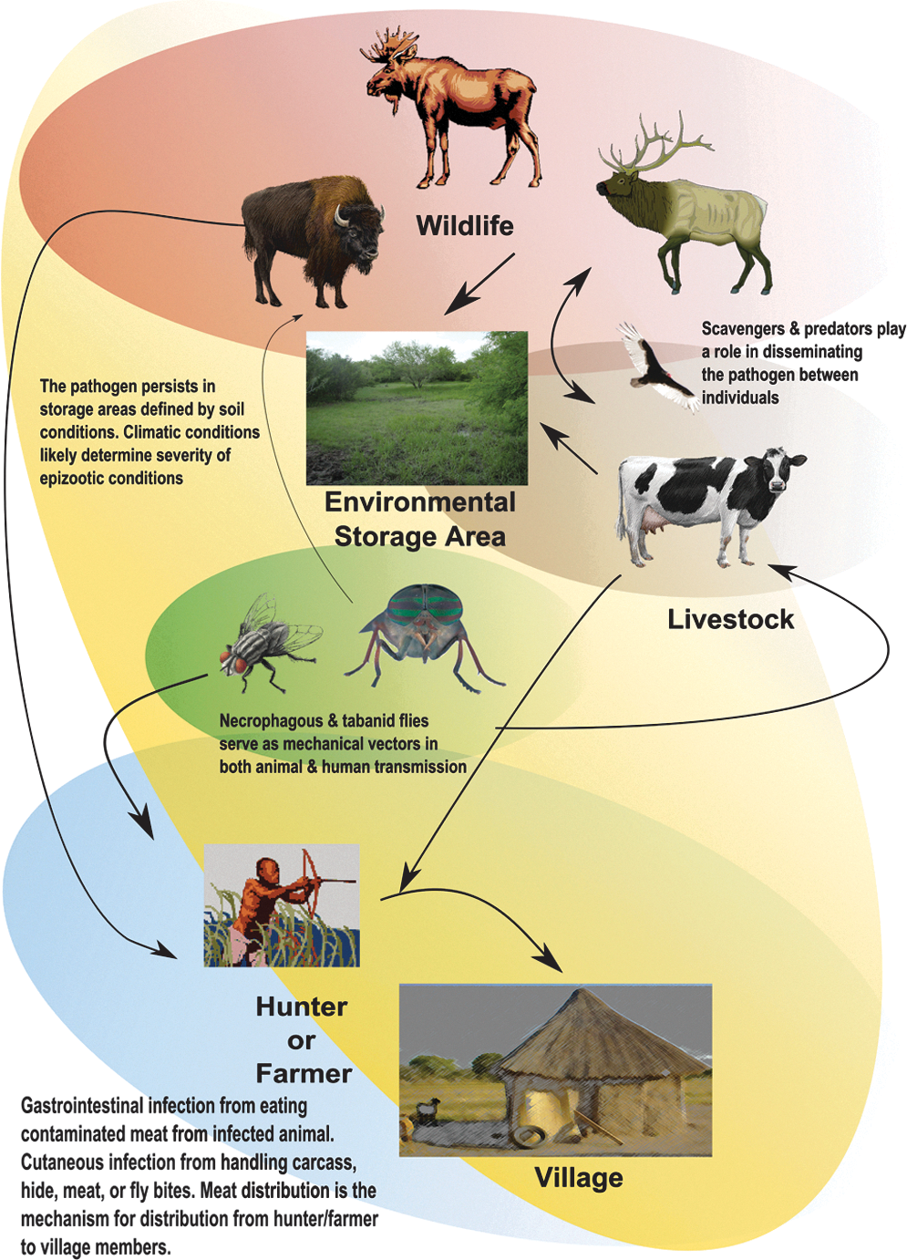
Anthrax is an obligate spillover pathogen for which cases are associated with direct interactions with the environment where the pathogen is sustained. Environmental and seasonal changes associated with bacterial storage areas are the primary drivers of epidemics, with human cases most likely directly linked to animal cases.

Ebola

Ebola hemorrhagic fever is an emerging zoonotic viral disease in West and Central Africa causing severe disease and high mortality in humans. Viral transmission is extremely complex, and both the behavior of individuals and multiple coupling points of transmission between species influence pathogen dynamics. Pathogen transmission to the human host appears to result from direct contact with infected wildlife species through the handling and eating of bush meat (duiker, primates, and bats; Leroy et al. 2009), a culturally-limiting behavior, or ingestion of fruit contaminated with Ebola-infected bat saliva (Leroy et al. 2009). Although the host spectrum and reservoir of infection have not been determined conclusively, three bat species are considered putative virus reservoirs (Leroy et al. 2005). There can be limited onward transmission in humans (e.g., person-to-person transmission), mainly resulting from close contact with blood, secretions, or tissues of infected individuals (Groseth et al. 2007). Public health responses are normally adequate to control and eliminate the outbreak in the human host population. Successful spillover of the pathogen appears to be a complex process involving a number of coupled networks (bat, fruiting trees, gorillas, duikers, and humans), and seasonal drivers (Pinzon et al. 2004), linking the human host to the virus reservoir (Fig. 2).

FIG. 2.

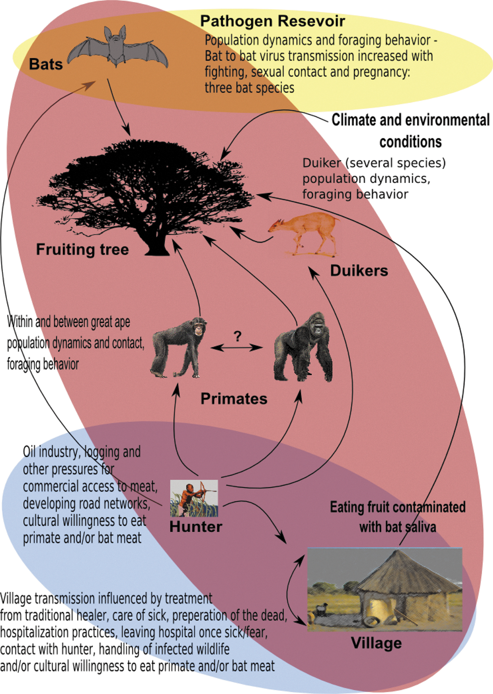
Ebola is an emerging zoonotic disease for which spillover dynamics appear to include up to four coupled systems. Population dynamics and seasonal influences appear to be the primary drivers of the process of pathogen invasion.

Using Ebola, a complex zoonotic pathogen with both spillover and onward transmission in humans, we illustrate schematically (in Figs. 4, 6, and 7) the application of three transmission modeling techniques and the general interpretation of the system that is identified with each approach. We also contrast the application of these techniques using our anthrax example, for which only spillover transmission is identified.

Recognizing Patterns in Disease Outbreaks

Ecological niche modeling

An important first step in understanding disease occurrence is the recognition of the spatial patterns in disease occurrence underlying phenomena important in zoonotic disease transmission. Predictive ecological niche modeling (ENM) is increasingly being used to predict the geographic distribution of multiple zoonotic pathogens and parasites, and to investigate and identify important factors associated with outbreak/case locations (Adjemian et al. 2006; Blackburn et al. 2007; Williams and Peterson 2009), and related ecological conditions (Blackburn 2006; Rogers 2006; Joyner 2010; Mullins et al. 2011). ENM is the process of identifying non-random relationships between known species occurrence locations (here the pathogen/parasite, host, reservoir, or vector), and climatic or environmental variables derived from interpolated ground or remotely sensed satellite data (Blackburn 2010). These data are analyzed through either genetic pattern-matching algorithms, such as the Genetic Algorithm for Rule-set Prediction (GARP) (Stockwell and Peters 1999), or statistical modeling, such as logistic regression (McPherson et al. 2004), discriminant function (Rogers 2006), or probability-based algorithms, such as MaxEnt (Phillips et al. 2006). The goal of such efforts is to model relationships between climatic/environmental conditions and occurrences in variable space, and to apply those to the geography to produce presence/absence maps for the target species being modeled (Blackburn 2010; Fig. 3). ENM has been applied to a wide range of taxa, including disease vectors (Peterson et al. 2002; Randolph et al. 2002; Adjemian et al. 2006; Rogers 2006; Holt et al. 2009), hosts (Peterson et al. 2002; Williams et al. 2008; Williams and Peterson 2009), and pathogens (Ron 2005; Blackburn et al. 2007). Across these examples, ENM-based approaches have been employed to directly map the potential distribution of the target species (host, vector, reservoir, or pathogen) to better understand the disease system. This concept is described in further detail elsewhere (Peterson 2007; Blackburn 2010).

FIG. 3.

In the ecological niche modeling approach, environmental data and disease (pathogen, host, or vector) occurrence data are combined in a niche theory framework to model the multi-variate space where the species is likely to be present. This modeled relationship is then applied to the landscape pixel-by-pixel to identify all regions where the species may be present. Successful models of the species on the known geography can be projected onto novel landscapes or the known landscape in future time periods to evaluate unknown regions or climate-related changes in distribution (NDVI, Normalized Difference Vegetation Index).

Broadly, ENM approaches can be divided into two major groups: presence-only and presence-absence models. In presence-only models (Pearce and Boyce 2006), species occurrence data are provided by the researcher, and absence data (commonly referred to as “background data”) are randomly drawn from the larger study area (Stockwell and Peters 1999), or user-defined subsets of the background (e.g., Phillips et al. 2009). In presence-absence models (Brotons et al. 2004), the user defines the locations on the landscape where the species is known to be present and absent. Across the literature there are strong arguments for both modeling approaches. However, it is not uncommon to develop ENM experiments from idiosyncratic data from a wide range of sources, such as disease reports, historical health records, and ongoing surveillance. In such cases, it is difficult to accurately determine species' absence, so presence-only models may be more appropriate. It is important to determine if such data sets reflect true absence (i.e., where the species is absolutely not present), versus where sampling efforts failed to detect the presence of the species (Anderson 2003). In this latter case, one must consider whether the species is truly absent from some portion of the landscape, or whether issues such as season of sampling effort or sampling technique may exclude individuals from collection/detection (Carlson and Cortés 2003). In the case of infectious diseases, it is also important to consider the sensitivity of diagnostic procedures and laboratory competency. On the one hand, presence-only modeling approaches may capitalize on available known disease occurrence locations from a wide variety of sources. At the same time, such approaches may bias ecological estimates towards presence points (Phillips et al. 2009). Presence-absence modeling approaches may overcome of some of these issues. However, following Brotons and associates (2004), presence/absence models may be most appropriate when confidence in absence locations can be determined. In disease studies, case-control studies or accurate surveillance may be used to provide such estimates of absence.

The ENM process is generally completed in two steps (Fig. 3). First, relationships between species' occurrences and climatic/environmental data are modeled in variable space (i.e., the combination of variable ranges that are available on the selected landscape for modeling). These relationships are captured as either logic strings, called rules in GARP, or direct formulas (such as logistic regression functions). The relationships derived are then applied to the landscape (in a global information system [GIS]), to “project” those relationships onto the geography of the area of interest in the form of binary presence/absence (in GARP), or cumulative probabilities of presence (in MaxEnt). Recently, GARP rules have been used to build and graph climatic envelopes for a specific genetic sub-lineage of Bacillus anthracis in Kazakhstan, compared to models built from larger data sets representing outbreaks regardless of genotype (Mullins et al. 2011). This process also allows the user to project models onto landscapes where occurrence data are unavailable, such as when surveillance or reporting are lacking (Blackburn 2010), or onto the same landscape in future time periods to evaluate the effects of climate change (Holt et al. 2009; Blackburn 2010; Joyner et al. 2010).

It is important to realize that geographic outputs from any ENM experiment are a prediction of the potential presence or absence of the target species. ENM predictions do not provide a measure of pathogen, host, or reservoir population size or density. Also, when selecting an appropriate ENM tool, it is important to realize that the extent of the predicted geographic space will differ relative to the nature of the niche space being estimated (Blackburn 2010). The body of literature related to the application of specific niche concepts to ENM is large and not without conflict. As primers, we refer readers to several key articles on niche definitions as applied to ENM, and issues associated with the differentiation of the fundamental and realized niche (McNyset 2005; Soberón and Nakamura 2009; Blackburn 2010). We also recommend the work of Phillips and associates (2006), for comments on discriminating between the two niche types with presence-only models. Clearly, differences in predictions can have implications for management and outbreak control activities. Over-prediction of the range of a pathogen may not appropriately define key areas at risk, while under-prediction may lead to gaps in surveillance. While it has been suggested that one tool may outperform the other (Elith et al. 2006), it is more appropriate to employ an exploratory approach, in which multiple models are tested and outcomes are evaluated (Peterson et al. 2008), in light of the objectives of the study.

Relative to the two disease examples used here, ENM can be used to define the potential spatial extent of the pathogen (anthrax), or occurrence of disease in a target host (Ebola). While the transmission dynamics of anthrax are not fully understood, there is some consensus on the environmental conditions that support B. anthracis spore survival (Hugh-Jones and Blackburn 2009). ENM has been employed to map the potential distribution of B. anthracis in the contiguous United States (Blackburn et al. 2007), and Kazakhstan (Joyner et al. 2010; Mullins et al. 2011). As an obligate spillover pathogen, these modeling efforts arguably delineate the geographic space associated with spillover, where the pathogen occurs and anthrax epidemics are likely to occur and recur (Blackburn 2010). In contrast, where reservoir host identification is uncertain, ENM can provide insight into the wildlife communities that might be associated and maintain the pathogen in the environment. For example, Peterson and colleagues (Peterson et al. 2004) modeled the potential distribution of filoviruses in Africa, such as Ebola, using human disease case data. These niche-based predictions were then used to delineate the spatial extent of disease occurrence in humans in order to identify potential common taxa that could serve as virus reservoirs for this group of related viruses (Peterson et al. 2004). In this latter case, ENM was used to model the spatial extent of disease transmission to delineate the possible geography where spillover can occur.

Patterns and spatial extents from ENMs can be used to inform animal and public health planning and surveillance strategy. Successful niche-based predictions can identify areas for targeted surveillance that may be at increased risk for disease occurrence (Blackburn 2010). This information can also improve passive surveillance systems by educating regional laboratories and clinics (human and animal) about potential disease risk in an area of interest. Disease control programs may also be informed by ENM outputs. Where vaccination might be applied to control disease, ecological inferences derived from ENM outputs could be used to target vaccine delivery, an often limited and expensive resource (Blackburn et al. 2007; Blackburn 2010). ENM outputs may also be used on a practical level to assist with parameterization of more complex compartmental or agent-based models. Geographic and ecological ranges derived from ENMs can provide variable value limits to constrain parameter estimates in other models.

Modeling Transmission Dynamics

Techniques like ENM can be used to identify spatial patterns associated with the environmental distribution of the pathogen and/or to generate hypotheses about variables/entities necessary for pathogen transmission. In both scenarios, however, understanding and estimating the dynamics of the system require other mathematical models and simulations to be applied, in order to take assessments further and evaluate mechanisms underlying a spillover event, and to develop quantitative predictions of the effectiveness of various control options (Anderson and May 1991; Diekmann and Heesterbeek 2000; Blackburn 2006).

Compartmental models

Traditionally, mathematical epidemiology has relied on compartmental models to describe infectious disease transmission between infected and susceptible hosts (Ross and Hudson 1917; Kermack and McKendrick 1932). While there are many variations, at its core this approach partitions the population into compartments based on disease state (frequently susceptible, exposed, infectious, and recovered, depending on the system), as well as other characteristics (e.g., demographics, location, and disease risk). The compartments are connected by differential equations describing their rates of exchange (e.g., rate of recovery describes proportions of infectious moving to recovered). Each compartment is assumed to be completely homogeneous, thus representing increased heterogeneity requires the inclusion of additional compartments. These compartments add equations representing the system, and require additional parameterization representing the levels of interaction between the different compartments. Once fully parameterized, these systems of equations can be analyzed to learn more about transmission dynamics. An attractive feature of this modeling approach is that it allows one to obtain analytical expressions for a number of interesting parameters, such as the numbers of infected, recovered, and susceptible individuals in a population at a given time. Compartment models can be used to model disease transmission and assess disease control options with various permutations as, for example, West Nile Virus in mosquitoes and birds (Wonham et al. 2004), Rift Valley Fever in mosquitoes and livestock (Gaff et al. 2007), and brucellosis in humans and animals (Zinsstag et al. 2005).

These models can become difficult to work with and solve for very complex zoonotic disease systems as Ebola, where multiple wildlife species are involved. A compartmental modeling approach is illustrated for Ebola in (Fig. 4), with classes of biologically-similar entities involved in disease transmission (bats, apes, and humans) grouped in the same layer (single-colored parallel planes). Note that within each entity class there can be several different compartments (pie charts illustrating the proportion of each disease state) representing different groups (both different species or within species groups). All members inside these compartments are assumed to be homogenous and to randomly mix. The arrows show the interactions between the different groups. While not an entity capable of infection, the green layer containing trees is included to highlight their role in modulating the interactions and opportunities for infections among the species. This also allows for the inclusion of the seasonal effects of rain (or other climatic events) to influence contact rates. As illustrated, the system would require four equations per compartment (13 in this representation), and each arrow represents a dependency between equations that would need to be considered and parameterized. A compartmental modeling approach would soon become intractable when applied to the full-coupled dynamics of Ebola viral transmission (Fig. 5).

FIG. 4.

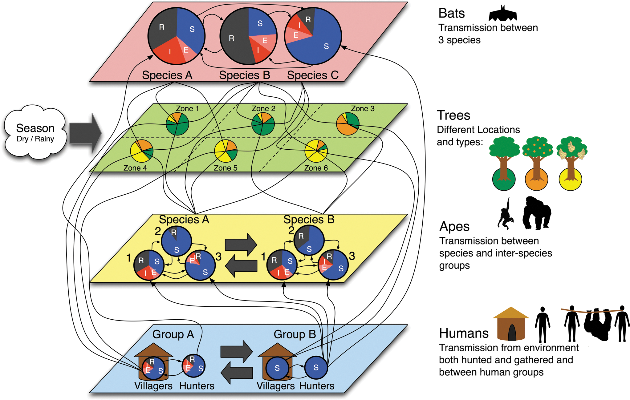
In the compartmental approach, each entity or interaction in Ebola viral transmission must be partitioned into a compartment (S, susceptible; E, exposed; I, infectious; R, recovered). The combination of lines across all layers and compartments necessitates a single equation. Parameterizing and solving these equations becomes difficult, and therefore limits model resolution and complexity.

FIG. 5.

A compartmental model is often used when the average characteristic patterns of the population or group are equivalent to individual level attributes (A). However, when population level patterns are no longer equivalent to individual level detail, and it is the individual level characteristics that are needed to derive key aggregate population level patterns (B), an agent-based model (ABM) will increasingly be required. Thus the more individual characteristics deviate or are suspected to deviate from population level patterns, the more complex the modeling requirements become (arrow at right).

While stochastic approaches (for which random elements can influence the process) are possible when using compartmental models, these models have a specified number of compartments that an individual can move into established a priori. This constrains the ability of the model to capture unexpected combinations of outcomes, and the cascading and interacting nature of events that can result in pathogen spillover from wildlife to humans (Smieszek et al. 2009). Additionally, the level of detail (e.g., resolution) of this approach is determined by its actual structure (and is thus limited by the model builder), making it difficult to incorporate rich data sets consumed and produced by techniques like ENM.

The assumption of homogenous mixing of hosts identified in compartmental models can be problematic when applied to the complex behavior and ecology of most wildlife species and may impact the results, elevating or artificially reducing parameter estimates depending on the true dynamics of the system (Meyers et al. 2005). Notwithstanding these limitations, the simplicity and computational tractability of this approach makes it an attractive choice if aggregate data can adequately represent individual level influences on disease transmission dynamics (Fig. 5). The compartmental modeling approach is capable of approximating the dynamics of many complex real-world systems involving wildlife species with model behavior well understood, as for example, the modeling of West Nile Virus cross-infection between birds and mosquitoes (Wonham et al. 2004).

When population level patterns are no longer equivalent to individual level detail and it is the individual level characteristics that are needed to derive key aggregate population level patterns, a patch or agent-based model (ABM) will increasingly be required. Thus the more individual characteristics deviate or are suspected to deviate from population-level patterns, the more complex the modeling requirements can become (Fig. 6). This increasing individual level resolution increases model complexity, data requirements, and related computational costs. As model complexity grows, there is the additional cost or risk associated with the increasing difficultly of understanding model behavior and relating this discretely to model structure.

FIG. 6.

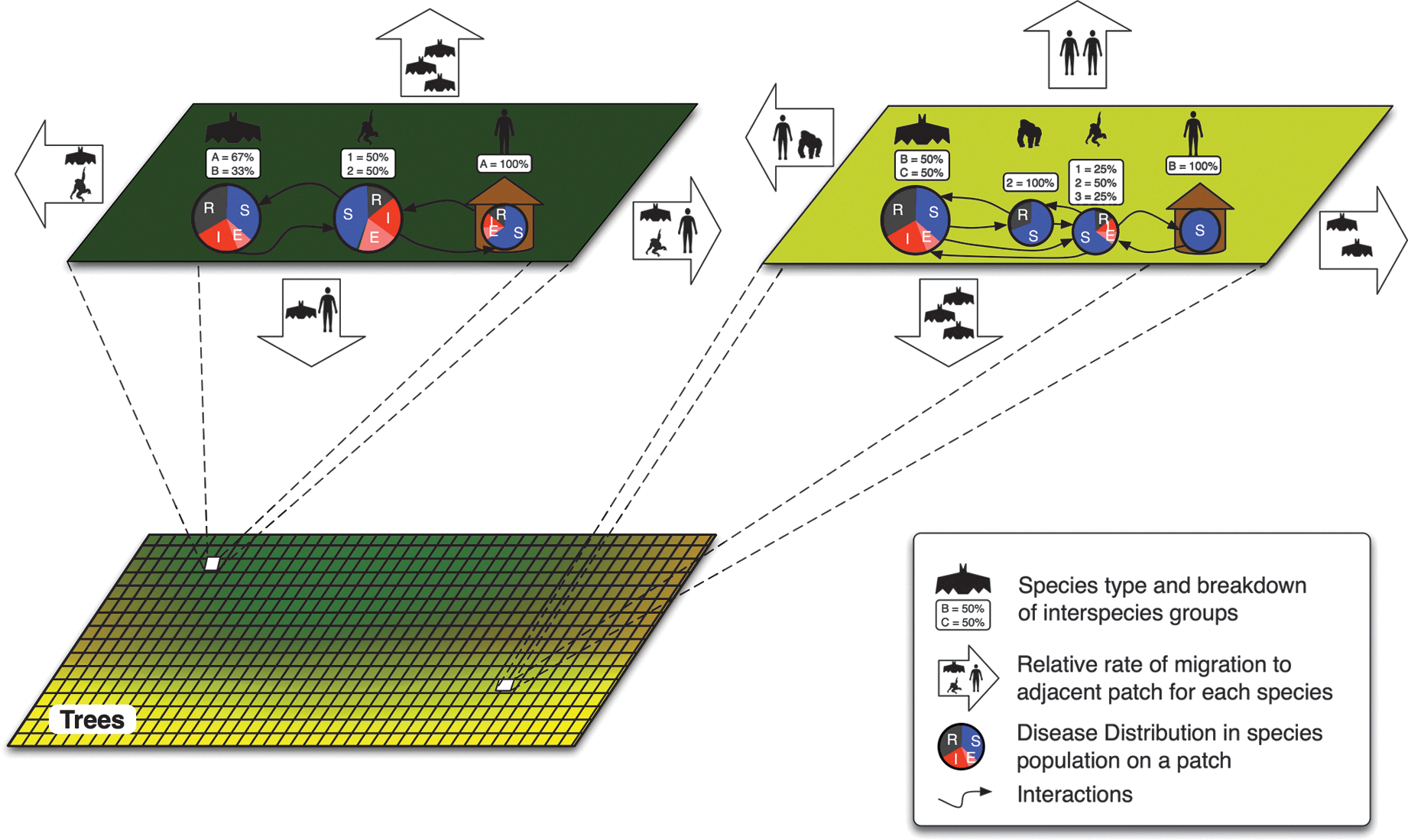
In the patch modeling approach, the environment is divided into patches to capture the heterogeneities from environmental factors. Within each patch a compartmental model, parameterized by these factors, is used to model the populations represented in this area. These compartmental models are also linked to adjacent patches to capture the population movements between the different patches (S, susceptible; E, exposed; I, infectious; R, recovered).

Patch modeling

Patch models, sometimes called metapopulation models, represent an extension of compartmental models that allows for a richer description of the characteristics of wildlife or human populations that can vary by location. Large physical areas are divided into separate patches that are configured with specific values for important characteristics that may vary over larger spatial scales (Riley 2007). Patch models have been applied to a variety of systems for which patch characteristics vary according to environmental-, pathogen-, and host-based heterogeneity, and interactions of the patches are defined by the modeler (Bauer et al. 2009; Tuite et al. 2011). Each patch contains a separate compartmental model that can interact with the surrounding patches in a predetermined manner. The assumption of homogeneity and uniform mixing in each patch persists in this approach, but inclusion of a limited spatial structure allows flexibility to accommodate high levels of heterogeneity (often using data drawn from the real-world to define the patches), yet still maintaining the computational tractability of compartmental models. An additional strength of the patch modeling approach can be seen in spatial structuring of patches, which can accommodate surveillance data that are often collected according to some administrative structure (e.g., states and hospitals). When the system includes wildlife hosts, species behavior or other ecological phenomena can be varied by region/patch (Gourley et al. 2008) to incorporate spatial variations. Patch models have been used successfully in evaluating the dynamics of important zoonoses, such as rabies, hantaviruses, and plague, for which landscape features separate populations into discrete patches, and spatial variations in pathogen and/or host dynamics are observed (McCormack and Allen 2007).

The patch model approach addresses the data resolution limitation of pure compartmental models. The framework of patches facilitates the inclusion of high-resolution data and organizes the interaction network. In Figure 6, in our Ebola example, the concentration of the different tree types (and thus inter-species interaction levels) is illustrated by the color gradient. Two individual patches are enlarged, showing the specific interactions between the entities and their relative levels of migration to adjacent patches. The yellow-green patch on the right (representing a higher concentration of banana trees) shows the interaction between different ape species, which increases the exposure for the currently disease-free group of humans. Accommodating high-resolution data helps make patch modeling more appropriate for capturing the conditions that can lead to spillover by incorporating greater heterogeneity by location. The mathematical framework still relies on coupled equations, which limits its ability to capture certain random effects and heterogeneities that can occur in the real system (Smieszek et al. 2009).

Agent-based modeling

Agent-based models (ABM) differ from compartmental models in that the system allows for individual heterogeneity, and important characteristics are assigned to the individual agents (Gilbert 2008). While there is wide variation, these agents generally represent individual entities in the system (e.g., human and/or wildlife population members and the elements of the environment). The model consists of the agents, the environment where the agents reside, and the rules that govern their dynamics. This basic framework supports the representation of very simple systems to very complex systems, an important flexibility that can be directed at understanding zoonotic disease emergence from wildlife. Agents can be richly described with many different characteristics, and many different classes of agents can be created (Epstein 2009). This synthetic environment provides opportunities for the agents to interact, and explicit inclusion of characteristics that can influence the type of interactions that can occur. The interaction rules define the dynamics of the interactions themselves, both what constitutes an interaction as well as its consequences. To represent more complex systems, the environments can be more richly detailed, as for example with the inclusion of detailed GIS-derived data (Kennedy et al. 2009). Interaction rules can be made to depend on characteristics of the environment and the agents themselves. For instance, the addition of age to an agent can correspondingly change how that agent moves over the environment, as well as change the agent's behavior (where a wildlife host seeks and how it obtains food in the system, territorial defense, reproduction, dominance interactions, immigration, and emigration). This induces a change in the interactions with others of the same or different species, humans in the system, and thus the potential for pathogen exposure and spillover (Fig. 7).

FIG. 7.

In an agent-based approach, individual behaviors and interactions can be represented across multiple coupled networks. These interactions can induce changes in the entities, which can, in turn, change which entities they interact with, and the nature of the interactions themselves.

ABMs can accommodate very complex dynamics since the interaction rules of each agent can depend on the current state of other dynamic processes (i.e., disease state of the agent, characteristics of the environment, or behaviors of the other agents). This allows infrequent events, such as pathogen spillover, to cascade through the different webs of interactions represented in the model, mirroring the often complex non-linear dynamics of zoonotic disease emergence. By capturing these cascades, the model can better elucidate the causative events rather than simply statistically correlate the behaviors of groups with a triggering event. This is a crucial difference and one that makes this representation most appealing in the study of zoonotic disease emergence. Individual-based network models for studying epidemics may qualitatively change the kind of scientific questions that one can study, and the scale of inquiry from cellular to population dynamics (Segovia-Juarez et al. 2004; Billari 2006; Young et al. 2008; Epstein 2009). In addition, this approach requires a procedural approach to representing the system, which forces a more explicit description of all elements of the model.

While ABM models offer an appealing mechanism for evaluating individual level attributes, behavior, and social networks in zoonotic pathogen transmission dynamics, it is often true that aggregate population information is more than adequate to answer the question posed, and inclusion of individual level detail in is not necessary. For example, anthrax transmission dynamics may be adequately captured with the compartmental approach.

ABM or patch approaches might provide an important hypothesis-testing tool for addressing incompletely understood transmission dynamics, by allowing a simulated exploration of conditions that have not been empirically assessed or tested. For example, ABMs might provide insight into the role of vectors in anthrax transmission, such as necrophagous fly contamination of vegetation (Blackburn 2010), and biting fly abundance (Blackburn 2006). Likewise, ABMs may be useful for testing hypotheses about host interactions that lead to inter-specific anthrax spillover. For example, Dragon and associates (Dragon et al. 1999) suggested that moose cases identified late in a wood bison epizootic were likely the product of mass contamination from a high number of bison cases. An ABM approach that studies both species might be useful for studying these interactions.

Caveats Associated with Zoonoses Involving Wildlife

The role of domestic animals in emerging zoonoses is generally better understood than that of wildlife, and is certainly more suitable for controlled studies, whereas essential data for wildlife may be lacking. When emerging zoonoses involve wildlife alone (Ebola), or are due to domestic animal spillover dynamics (anthrax), the complexity of the system increases dramatically. In most cases, high-resolution detail regarding relevant local ecological, behavioral, and demographic data are not available for single or multiple wildlife species involved in putative or known transmission dynamics (e.g., bats, duiker, gorillas, chimps for Ebola). There is the increasing, yet unfortunate, recognition that the characterization of a species and pathogen can vary substantially by location, and understanding the host and/or pathogen in one system may lead to little or erroneous insight into another system where the same pathogen and host occur (Proffitt et al. 2011).

Modeling of pathogen transmission in wildlife-associated zoonotic disease is also influenced by how transmission scales with population size and density of a particular species (one or more McCallum et al. 2001), attributes are expected to change in wildlife populations both spatially and temporally (Hudson et al. 2002). The assumption of homogenous mixing (e.g., patch and compartmental models) can be particularly problematic where wildlife hosts are involved, as complex spatial and social structuring of host populations (e.g., territoriality, dominance, breeding behavior, and social system) often occurs (Lloyd-Smith et al. 2005). Infectious disease itself can in turn influence and modify population dynamics in wildlife systems. As an example, reproductive compensation has been identified in the Tasmanian devil (Sarcophilus harrisii) as an apparent compensatory response to disease-driven population declines associated with devil facial tumor disease. Diseased mothers also had greater numbers of female offspring than uninfected mothers, increasing the spectrum of host demographic responses to infectious disease (Lachish et al. 2009).

Reservoir dynamics in wildlife populations can also be complex, involving various host species and populations, the characterization of which may change both temporally and spatially (Haydon et al. 2002). These variations can be extreme where a species may act as a primary reservoir or maintenance host in a particular system, but a non-maintenance host involved in pathogen spillover in another. Such is the case with brucellosis in elk (Cervus elaphus), acting as a primary maintenance host in the greater Yellowstone area (Cross et al. 2010), while the same animal in Spain serves as a species involved in pathogen transmission only when it is unable to maintain the pathogen in the absence of domestic livestock (Serrano et al. 2011). Often there is simply insufficient knowledge about the specific role of the species in maintaining the pathogen in the system (e.g., African buffalo [Syncerus kaffer] and brucellosis; Alexander et al. 2012). The potential for multiple unknown alternate host species presents a particular challenge in characterizing these complex systems (e.g., Ebola, Feldmann et al. 2004; Marburg virus, Swanepoel et al. 2007; and Mycobacterium mungi, Alexander et al. 2010).

Human culture and behavior can influence the risk of exposure to wildlife-associated zoonoses (Alexander and McNutt 2010). For example, use of bush meat (meat originating from wildlife), and the risk of human exposure to bush meat–associated pathogens (e.g., brucellosis and Ebola), will vary among communities and families based on traditions that influence meat preferences by species, processing practices, and distribution of animal meat and products among family members and elders (Alexander et al. 2012). These cultural drivers of zoonotic pathogen exposure and invasion may be critical to model structure and to capture pathogen spillover dynamics at the human–wildlife interface.

Management of zoonoses in wildlife is another area of complexity, given sufficient economic or public health interest in pursuing eradication, or more commonly, control. Host population thresholds for pathogen invasion (threshold population for invasion), and persistence (critical community size), are central to disease control actions such as culling and vaccination. However, these thresholds are difficult to apply in wildlife populations, and do not account for sources of population demographic heterogeneity, such as seasonal births and compensatory reproduction as discussed above. In many cases, disease eradication is often impossible, and control may not be effective when derived from such threshold targets (Lloyd-Smith et al. 2005). Control activities such as vaccination or culling may also have unintended negative effects on the host population and pathogen transmission dynamics, as seen with badger culling for tuberculosis control. In this instance, disruption of badger social groups in response to culling not only increased dispersal rates, but infected badgers also dispersed further than uninfected badgers (Pope et al. 2007).

Conclusions

The decision on the specific class of models to apply to a particular zoonotic disease outbreak involving wildlife will depend on the following criteria: (1) the computational resources needed to execute the models and analyze the data produced by the models; (2) the scale and resolution of empirical data to calibrate and initialize model parameters; (3) the time needed to construct the models; (4) the time needed for model execution, testing, and analysis; (5) the kinds of analysis one is interested in; and (6) the complexity and characteristics of the system under study. Where mathematical, algorithmic, and software expertise limits appropriate model application, scientists must seek out the appropriate collaborations to secure the necessary expertise. Not all modeling tools are the same, and it is important that the right tool is used for the right problem. A lack of knowledge should not be a barrier to the appropriate use of the modeling toolbox for zoonotic disease investigations. It is important to identify and incorporate the system complexity inherent and fundamental to the cascade of events that result in zoonotic disease invasions involving wildlife hosts (Lloyd-Smith et al. 2009).

Mathematical models have been used as an important tool in our war against zoonotic disease. There is an increasing need for these techniques to be more broadly understood by wildlife and human health researchers who are not modelers. Effective management of zoonotic disease threats will require the active collaboration of wildlife and animal health professionals with public health specialists, both empiricists and theoreticians. This will assist in addressing knowledge gaps and operational barriers that currently impede the successful surveillance and management of emerging zoonotic diseases.

Summary

• Mathematical models are important tools in the study of zoonotic disease, but there is a need for increased computational focus on the coupled dynamics of human and wildlife systems that underlie the process of zoonotic disease emergence, and incorporation of heterogeneities inherent in these systems.

• Ecological niche modeling can be an important first step to understanding the geographic potential of a disease, either directly through modeling the pathogen (e.g., Bacillus anthracis), or the system (e.g., Ebola). Niche-based predictions can be used to inform other modeling approaches, and to describe the multivariate space where zoonoses and spillover events are most likely to occur. Projecting onto unknown landscapes or future time periods allows modelers to speculate about broader geographies or climate change.

• Compartmental models of disease transmission can help map out the parameter space of the problem, and provide estimates of the drivers of spillover events and possible outcomes following spillover.

• Patch models incorporate high-resolution data sources that vary by location into a compartmental framework, thus providing an opportunity to find specific combinations of conditions that can lead to spillover.

• Agent-based models accommodate high-resolution data down to the individual level, and incorporate stochasticity in a way that can more clearly elucidate the roles of the different conditions that lead to spillover.

• Increased model complexity and level of data resolution do not ensure higher-quality or more credible results.

• The more individual characteristics deviate or are suspected to deviate from population level patterns, the more complex the modeling requirements become, and the greater the need to incorporate these individual level attributes in modeling approaches.

Footnotes

Acknowledgments

This work was partially supported by National Science Fund (NSF) HSD grant SES-0729441, National Institutes of Health MIDAS project 2U01GM070694-7, NSF PetaApps grant OCI-0904844, DTRA15 R&D grant HDTRA1-0901-0017, DTRA CNIMS grant HDTRA1-07-C-0113, NSF CNH 114953, and NSF grant CNS-0845700.

Author Disclosure Statement

No competing financial interests exist.

References

Adjemian

, Girvetz

, Beckett

et al. Analysis of Genetic Algorithm for Rule-Set Production (GARP) modeling approach for predicting distributions of fleas implicated as vectors of plague, Yersinia pestis, in California. J Med Entomol, 2006; 43:93–103.

Alexander

, Blackburn

, Pesapane

et al. Buffalo, bush meat and the zoonotic threat of brucellosis in Botswana. PLoS One, 2012; 7:e23842.

Alexander

, Laver

, Michel

et al. The emergence of a previously unidentified Mycobacterium tuberculosis complex pathogen, M. mungi, sp nov. at the human-wildlife interface. Emerg Infect Dis, 2010; 16:1296–1299.

Alexander

, McNutt

. Human behavior influences infectious disease emergence at the human-animal interface. Front Ecol Environ, 2010.

Anderson

, May

. Infectious Diseases of Humans: Dynamics and Control. New York: Oxford, 1991; 757.

Anderson

. Real vs. artefactual absences in species distributions: tests for Oryzomys albigularis (Rodentia: Muridae) in Venezuela. J Biogeography, 2003; 30:591–605.

Bauer

, Beauchemin

CAA

, Perelson

. Agent-based modeling of host-pathogen systems: The successes and challenges. Information Sci, 2009; 179:1379–1389.

Beatty

, Scott

, Tsai

. Achieving sustainable global capacity for surveillance and response to emerging diseases of zoonotic origin: workshop report. Natl Academy Press, 2008.

Billari

. Agent-based computational modelling: applications in demography, social, economic and environmental sciences. Physica Verlag, 2006.

10.

Blackburn

, Curtis

, Hadfield

et al. Confirmation of Bacillus anthracis from flesh-eating flies collected during a West Texas anthrax season. J Wildlife Dis, 2010; 46:918.

11.

Blackburn

. Evaluating the spatial ecology of anthrax in North America: Examining epidemiological components across multiple geographic scales using a GIS-based approach. Department of Geography and Anthropology. Baton Rouge: Louisiana State University, 2006; 141.

12.

Blackburn

. Integrating geographic information systems and ecological niche modeling into disease ecology: a case study of Bacillus anthracis in the United States and Mexico. Emerging and Endemic Pathogens: Advances in Surveillance, Detection, and Identification. O'Connell

, Sulakvelidze

, Bakanidze

. New York: Springer, 2010; 59–88.

13.

Blackburn

, McNyset

, Curtis

et al. Modeling the geographic distribution of Bacillus anthracis, the causative agent of anthrax disease, for the contiguous United States using predictive ecologic niche modeling. Am J Trop Med Hyg, 2007; 77:1103.

14.

Brotons

, Thuiller

, Araújo

, Hirzel

. Presence-absence versus presence-only modelling methods for predicting bird habitat suitability. Ecography, 2004; 27:437–448.

15.

Bryan

, Pinner

, Berkelman

. Emerging infectious diseases in the United States: improved surveillance, a requisite for prevention. Ann NY Acad Sci, 1994; 740:346–361.

16.

Carlson

, Cortés

. Gillnet selectivity of small coastal sharks off the southeastern United States. Fisheries Res, 2003; 60:405–414.

17.

Cross

, Cole

, Dobson

et al. Probable causes of increasing brucellosis in free-ranging elk of the Greater Yellowstone Ecosystem. Ecological Appl, 2010; 20:278–288.

18.

Diekmann

, Heesterbeek

. Mathematical Epidemiology of Infectious Diseases. Chichester: John Wiley and Sons, 2000.

19.

Dragon

, Elkin

, Nishi

et al. A review of anthrax in Canada and implications for research on the disease in northern bison. J Appl Microbiol, 1999; 87:208–213.

20.

Elith

, Graham

, Anderson

et al. Novel methods improve prediction of species' distributions from occurrence data. Ecography, 2006; 29:129–151.

21.

Epstein

. Modelling to contain pandemics. Nature, 2009; 460:687–687.

22.

Feldmann

, Wahl-Jensen

, Jones

et al. Ebola virus ecology: a continuing mystery. Trends Microbiol, 2004; 12:433–437.

23.

Gaff

, Hartley

, Leahy

. An epidemiological model of Rift Valley fever. Electronic J Differential Equations, 2007; 2007:1–12.

24.

Gilbert

. Agent-Based Models. Thousand Oaks, CA: Sage Publications, 2008.

25.

Gourley

, Liu

, Wu

. Spatiotemporal patterns of disease spread: Interaction of physiological structure, spatial movements, disease progression and human intervention. Structured Population Models Biol Epidemiol, 2008; 165–208.

26.

Groseth

, Feldmann

, Strong

. The ecology of Ebola virus. Trends Microbiol, 2007; 15:408–416.

27.

Halliday

JEB

, Meredith

, Knobel

et al. A framework for evaluating animals as sentinels for infectious disease surveillance. J Royal Soc Interface, 2007; 4:973.

28.

Haydon

, Cleaveland

, Taylor

et al. Identifying reservoirs of infection: a conceptual and practical challenge. Emerg Infect Dis, 2002; 8:1468–1473.

29.

Holt

, Salkeld

, Fritz

et al. Spatial analysis of plague in California: niche modeling predictions of the current distribution and potential response to climate change. International J Health Geographics, 2009; 8:38.

30.

Hudson

, Rizzoli

, Grenfell

et al. Ecology of Wildlife Diseases. Oxford: Oxford University Press, 2002.

31.

Hugh-Jones

, Blackburn

. The ecology of Bacillus anthracis. Mol Aspects Med, 2009; 30:356–367.

32.

Hugh-Jones

, De Vos

. Anthrax and wildlife. Revue scientifique et technique (International Office of Epizootics), 2002; 21:359.

33.

Jones

, Patel

, Levy

et al. Global trends in emerging infectious diseases. Nature, 2008; 451:990–993.

34.

Joyner

. Ecological niche modeling of a zoonosis: a case study using anthrax and climate change in Kazakhstan geography. Gainesville: University of Florida, 2010; 150.

35.

Joyner

, Lukhnova

, Pazilov

et al. Modeling the potential distribution of Bacillus anthracis under multiple climate change scenarios for Kazakhstan. PloS One, 2010; 5:e9596.

36.

Kennedy

, Lane

, Arifin

SMN

et al. A GIS aware agent-based model of pathogen transmission. Int J Intelligent Control Syst, 2009; 14:51–61.

37.

Kermack

, McKendrick

. Contributions to the mathematical theory of epidemics. II. The problem of endemicity. Proc Royal Soc Lond Series A, 1932; 138:55.

38.

Lachish

, McCallum

, Jones

. Demography, disease and the devil: life and history changes in a disease-affected population of Tasmanian devils (Sarcophilus harrisii) J Animal Ecol, 2009; 78:427–436.

39.

Leroy

, Epelboin

, Mondonge

et al. Human Ebola outbreak resulting from direct exposure to fruit bats in Luebo, Democratic Republic of Congo, 2007. Vector-Borne Zoonotic Dis, 2009; 9:723–728.

40.

Leroy

, Kumulungui

, Pourrut

et al. Fruit bats as reservoirs of Ebola virus. Nature, 2005; 438:575–576.

41.

Levin

, Grenfell

, Hastings

et al. Mathematical and computational challenges in population biology and ecosystems science. Science, 1997; 275:334.

42.

Lloyd-Smith

, Cross

, Briggs

et al.

Should we expect population thresholds for wildlife disease?

Trends Ecol Evolution, 2005; 20:511–519.

43.

Lloyd-Smith

, George

, Pepin

et al. Epidemic dynamics at the human-animal interface. Science, 2009; 326:1362.

44.

McCormack

, Allen

LJS

. Multi-patch deterministic and stochastic models for wildlife diseases. J Biological Dynamics, 2007; 1:63–85.

45.

McNyset

. Use of ecological niche modelling to predict distributions of freshwater fish species in Kansas. Ecol Freshwater Fish, 2005; 14:243–255.

46.

McPherson

, Jetz

, Rogers

. The effects of species' range sizes on the accuracy of distribution models: ecological phenomenon or statistical artefact? J Applied Ecol, 2004; 41:811–823.

47.

Meyers

, Pourbohloul

, Newman

MEJ

et al. Network theory and SARS: predicting outbreak diversity. J Theoretical Biol, 2005; 232:71–81.

48.

Morse

. Factors in the emergence of infectious diseases. Emerg Infect Dis, 1995; 1:7–15.

49.

Mullins

, Lukhnova

, Aikimbayev

et al. Ecological niche modelling of the Bacillus anthracis A1. a sub-lineage in Kazakhstan. BMC Ecol, 2011; 11:32.

50.

Pearce

, Boyce

. Modelling distribution and abundance with presence-only data. J Appl Ecol, 2006; 43:405–412.

51.

Peterson

, Bauer

, Mills

. Ecologic and geographic distribution of filovirus disease. Emerg Infect Dis, 2004; 10:40–47.

52.

Peterson

. Ecological niche modelling and understanding the geography of disease transmission. Vet Ital, 2007; 43:393–400.

53.

Peterson

, Papes

, Soberón

. Rethinking receiver operating characteristic analysis applications in ecological niche modeling. Ecological Modelling, 2008; 213:63–72.

54.

Peterson

, Sánchez-Cordero

, Beard

et al. Ecologic niche modeling and potential reservoirs for Chagas disease, Mexico. Emerg Infect Dis, 2002; 8:662.

55.

Peterson

, Carroll

, Mills

et al. Potential mammalian filovirus reservoirs. Emerg Infect Dis, 2004; 10:2073–2081.

56.

Phillips

, Anderson

, Schapire

. Maximum entropy modeling of species geographic distributions. Ecological Modelling, 2006; 190:231–259.

57.

Phillips

, Dudík

, Elith

et al. Sample selection bias and presence-only distribution models: implications for background and pseudo-absence data. Ecological Applic, 2009; 19:181–197.

58.

Pinzon

, Wilson

, Tucker

et al. Trigger events: enviroclimatic coupling of Ebola hemorrhagic fever outbreaks. Am J Tropi Med Hyg, 2004; 71:664.

59.

Pope

, Butlin

, Wilson

et al. Genetic evidence that culling increases badger movement: implications for the spread of bovine tuberculosis. Molec Ecol, 2007; 16:4919–4929.

60.

Proffitt

, Gude

, Hamlin

et al. Elk distribution and spatial overlap with livestock during the brucellosis transmission risk period. J Appl Ecol, 2011; 48:471–478.

61.

Rabinowitz

, Gordon

, Holmes

et al. Animals as sentinels of human environmental health hazards: an evidence-based analysis. EcoHealth, 2005; 2:26–37.

62.

Randolph

, Chemini

, Furlanello

et al. The ecology of tick-borne infections in wildlife reservoirs. Ecol Wildlife Dis, 2002; 119–138.

63.

Remsen

, Good

. Misuse of data from mist-net captures to assess relative abundance in bird populations. Auk, 1996; 381–398.

64.

Riley

, Fraser

, Donnelly

et al. Transmission dynamics of the etiological agent of SARS in Hong Kong: impact of public health interventions. Science, 2003; 300:1961.

65.

Riley

. Large-scale spatial-transmission models of infectious disease. Science, 2007; 316:1298.

66.

Rogers

. Models for vectors and vector-borne diseases. Adv Parasitol, 2006; 62:1–35.

67.

Ron

. Predicting the distribution of the amphibian pathogen Batrachochytrium dendrobatidis in the New World 1. Biotropica, 2005; 37:209–221.

68.

Ross

, Hudson

. An application of the theory of probabilities to the study of a priori pathometry. Part II. Proc Roy Soc London Series A, 1917; 93:212.

69.

Segovia-Juarez

, Ganguli

, Kirschner

. Identifying control mechanisms of granuloma formation during M. tuberculosis infection using an agent-based model. J Theoretical Biol, 2004; 231:357–376.

70.

Serrano

, Cross

, Beneria

et al. Decreasing prevalence of brucellosis in red deer through efforts to control disease in livestock. Epidemiol Infect, 2011; 1:1–5.

71.

Smieszek

, Fiebig

, Scholz

. Models of epidemics: when contact repetition and clustering should be included. Theor Biol Med Model, 2009; 6:11.

72.

Smith

, DeVos

, Bryden

et al. Bacillus anthracis diversity in Kruger National Park. J Clin Microbiol, 2000; 38:3780.

73.

Soberón

, Nakamura

. Niches and distributional areas: concepts, methods, and assumptions. Proc Natl Acad Sci, 2009; 106:19644–19650.

74.

Stockwell

, Peters

. The GARP modelling system: problems and solutions to automated spatial prediction. Int J Geographical Information Sci, 1999; 13:143–158.

75.

Swanepoel

, Smit

, Rollin

et al. Studies of reservoir hosts for Marburg virus. Emerg Infect Dis, 2007; 13:1847.

76.

Tuite

, Tien

, Eisenberg

et al. Cholera epidemic in Haiti, 2010: Using a transmission model to explain spatial spread of disease and identify optimal control interventions. Ann Intern Med, 2011; 154:593.

77.

Turnbull

, Böhm

, George

, Chizyuka

. Guidelines for the Surveillance and Control of Anthrax in Humans and Animals, 4th. WHO: Geneva, 2008; 219.

78.

Williams

, Fasina

, Peterson

. Predictable ecology and geography of avian influenza (H5N1) transmission in Nigeria and West Africa. Transact Roy Soc Trop Med Hyg, 2008; 102:471–479.

79.

Williams

, Peterson

. Ecology and geography of avian influenza (HPAI H 5 N 1) transmission in the Middle East and northeastern Africa. Int J Health Geographics, 2009; 8:47.

80.

Wonham

, de-Camino-Beck

, Lewis

. An epidemiological model for West Nile virus: invasion analysis and control applications. Proc Roy Soc Lond Series B, 2004; 271:501.

81.

Woods

, Ospanov

, Myrzabekov

et al. Risk factors for human anthrax among contacts of anthrax-infected livestock in Kazakhstan. Am J Trop Med Hyg, 2004; 71:48.

82.

Yang

, Sugimoto

, Halloran

et al. The transmissibility and control of pandemic influenza A (H1N1) virus. Science, 2009; 326:729.

83.

Young

, Stark

, Kirschner

. Systems biology of persistent infection: tuberculosis as a case study. Nat Rev Microbiol, 2008; 6:520–528.

84.

Zinsstag

, Roth

, Orkhon

et al. A model of animal-human brucellosis transmission in Mongolia. Prevent Vet Med, 2005; 69:77–95.