Looking Forward by Looking Back: Using Historical Calibration to Improve Forecasts of Human Disease Vector Distributions

Abstract

Arthropod disease vectors, most notably mosquitoes, ticks, tsetse flies, and sandflies, are strongly influenced by environmental conditions and responsible for the vast majority of global vector-borne human diseases. The most widely used statistical models to predict future vector distributions model species niches and project the models forward under future climate scenarios. Although these methods address variations in vector distributions through space, their capacity to predict changing distributions through time is far less certain. Here, we review modeling methods used to validate and forecast future distributions of arthropod vectors under the effects of climate change and outline the uses or limitations of these techniques. We then suggest a validation approach specific to temporal extrapolation models that is gaining momentum in macroecological modeling and has great potential for epidemiological modeling of disease vectors. We performed systematic searches in the Web of Science, ScienceDirect, and Google Scholar to identify peer-reviewed English journal articles that model arthropod disease vector distributions under future environment scenarios. We included studies published up to and including June, 2014. We identified 29 relevant articles for our review. The majority of these studies predicted current species niches and projected the models forward under future climate scenarios without temporal validation. Historically calibrated forecast models improve predictions of changing vector distributions by tracking known shifts through recently observed time periods. With accelerating climate change, accurate predictions of shifts in disease vectors are crucial to target vector control interventions where needs are greatest.

Introduction

Rising concerns over environmental changes and their potential effects on disease prevalence require more extensive exploration of statistical modeling methods that can accurately predict future disease vector distributions (Mills et al. 2010, Tabachnick 2010). Satellite-based remote sensing and statistical geographic information tools continue to evolve at an extraordinary pace, providing continuous measurements of environmental factors at progressively finer spatial and temporal resolutions (Hay et al. 2000). As a result, increasingly accurate spatial models are being created using present-day data and are projected into future time periods to predict disease vector distributions under climate change scenarios (e.g., Tonnang et al. 2010). Although many of these models appear accurate across space, their predictions are often highly divergent through time (Araujo et al. 2005b, Pearson et al. 2006, Kharouba et al. 2009, Braunisch et al. 2013). The “temporal transferability” of these models—their ability to predict independent events through time correctly—is highly uncertain (Araujo and Guisan 2006).

The failure of the space-for-time assumption (Blois et al. 2013) imposes strong limits on the reliability of spatial models for temporal prediction. For example, nine modeling techniques used to forecast four South African plant species' distributions in 2030 predicted between a 92% loss to a 322% gain, but all models successfully described the current spatial distributions of these species (Pearson et al. 2006). Furthermore, environmental factors that correlate positively with species' distributions spatially may show the opposite relationship temporally. For example, models of Canadian butterfly species' richness showed a positive association with human population density spatially but a negative association temporally (White and Kerr 2006). Species distribution modeling methods range from logistic regression to highly specialized machine-learning techniques (Elith and Leathwick 2009), all of which have proven useful under different circumstances. Strong tests of model accuracy are critical to forecasting how changing environmental circumstances will alter the distributions of disease vectors through time.

Accurately projecting distributions of human disease vectors, such as those transmitting malaria, Lyme disease, dengue, and trypanosomiasis, is crucial because of their human health impacts and the related economic consequences of misdirected management interventions. Yet, predictions of future vector distributions often conflict. For example, models of Anopheles mosquito distributions, the vectors of the malaria parasite, across the Caribbean did not predict northern range expansions into the Gulf coastal region under warming climates by 2080, contradicting previous studies which predicted future expansions of malaria by as early as 2050 (Fuller et al. 2012a). Conflicting results of future vector distributions mislead control programs and practices that already pose substantial financial challenges for many developing countries (Martens et al. 1999, World Health Organization 2008). Technological advances are unlikely to permit predictions of future species distributions to be tested unambiguously; the definitive, but impractical, method for testing such models is to wait to compare predictions to actual events (Rastetter 1996, Algar et al. 2009). This does not mean that forecasting future species distributions and validating these methods lacks rigor. It does, however, underscore the need for strong validation methods to increase confidence that such models are reliable (Botkin et al. 2007).

There are extensive parallels between macroecological models, which predict species distributions over broad areas (e.g., regions and continents; see Brown and Maurer 1989, Kerr et al. 2007), and epidemiological models needed to predict changing vector distributions across comparable modeled areas. Both may use correlative and mechanistic methods for projecting changing species distributions (for a comparison of these two methods in vector modeling under future climates, see Fischer et al. 2014). Correlative models can include general linear models or use machine-learning techniques, such as maxent (Phillips et al. 2006), techniques from the Biomod modeling package, such as random forest analyses (Thuiller 2003), and genetic algorithms for rule-set production (Stockwell and Peters 1999) to relate species occurrence records to environmental factors and determine the area the species actually occupies (i.e., realized niche). Mechanistic models, or stochastic models coupled with habitat suitability or population models, use lab- and field-based measures of physiological traits (e.g., behavior, temperature tolerances, energy turnover) to determine all potential areas where the species may persist (i.e., fundamental niche) (Kearney and Porter 2009). Temporal macroecological models often seek to forecast future species distributions for the purposes of conservation (Trejo et al. 2011), invasive species (Sobek-Swant et al. 2012), or agriculture (Ureta et al. 2012); their forecasting and validation methods show considerable overlap with those predicting changing disease risk. Satellite remote-sensing tools provide a common array of baseline measurements for both fields that are revolutionizing statistical modeling in epidemiology (Hay et al. 2000) and macroecology (Kerr and Ostrovsky 2003) by improving detection of spatial and temporal variation in the biophysical determinants of species distributions. Consequent syntheses of techniques from both disciplines has led to the emergence of “eco-epidemiology,” “landscape epidemiology” (Pavlovsky 1966, Kitron 1998, Peterson 2006, Reisen 2010), “medical geography” (Meade and Earickson 2000), and “disease macroecology” (Keith et al. 2012).

In attempting to predict changes in species distributions through time, predictive models commonly share a straightforward approach. Generally, these models: (1) Use current environmental conditions to predict current disease vector distributions, (2) test the accuracy of the model by evaluating its fit to current spatial observations, and (3) project the model to a future time period by substituting anticipated environmental observations into the spatial model. Spatial validation, which improves confidence in model fit in the current time period, does not imply temporal reliability. To ensure the latter, analyses must be multitemporal (Kharouba et al. 2009). A validation technique that accounts for time (or historical calibration) is needed. Using this approach, models are constructed with observations from different time periods. These models are then projected either backward or forward into a time period with independent vector data to test their capacity to predict changing distributions through time. Historical calibration is likely the minimum requirement to establish confidence that these models can be used to forecast changes in vector distributions accurately (e.g., Kharouba et al. 2009, Rapacciuolo et al. 2014). This approach provides spatiotemporal tests of model reliability, rather than spatial tests followed by risky reliance on space-for-time assumptions.

Here, we review the critical field of forecasting future disease vector distributions under changing climate. First, we discuss the different methods used to validate the spatial models of present-day vector distributions. Next, we assess how these spatial models are projected into future time periods under different climatic scenarios. We then introduce the framework we call historical calibration for validation that is specific to temporal extrapolations in macroecology and may increase accuracy of forecasting models in epidemiology. While we focus on disease vectors that directly affect human health for this review, the assessment of the forecast and validation approaches can be applied across spatial scales and broadly among many focal species and hosts, such as livestock (e.g., for advances in forecast modeling of Culicoides midges and the bluetongue virus in livestock, see Acevedo et al. 2010 and Guichard et al. 2014).

Materials and Methods

We performed systematic searches in three databases for peer-reviewed literature: Web of Science (http://thomsonreuters.com/thomson-reuters-web-of-science), ScienceDirect (www-sciencedirect-com.web.bisu.edu.cn/), and Google Scholar (http://scholar.google.com). We restricted the search to English journal papers. We included studies published up to and including June, 2014. Each search varied depending on the search engine input options, but combined the following three sets of inputs: The first set used “either/or” for the projection methods “forecast*,” “climate scenario*,” “projection,” or “future”; the second set used “either/or” for the model types “correlative,” “mechanistic,” or “model”; the third set used “either/or” for the vector species “mosquito*,” “tsetse*,” “tick*,” or “sandfly*.” While the term “forecast” generally refers to predicting forward through time, relative to a baseline period (e.g., using historical data to predict present-day conditions) (Elith and Leathwick 2009), this review only examines papers forecasting future events. The initial searches yielded a total of 1082 papers. Studies were included if they predicted future vector distributions under changing climate or changing nonclimatic factors (e.g., land use). Therefore, we excluded studies that modeled disease cases instead of the arthropod vector itself (e.g., Naish et al. 2013). We included studies using future climate scenarios (e.g., general circulation models, or GCMs) and environmental changes proposed by the study (e.g., incremental increases in temperature). Both correlative and mechanistic models were included. Because the focus of this review is forecasting arthropod vectors that transmit diseases to humans, we excluded models of vectors that solely attack nonhumans, such as livestock. We also excluded nonarthropod vectors, such as rodents. On the basis of these inclusion and exclusion criteria, only 29 studies remained relevant as primary literature in the final review.

Results and Discussion

Validating spatial models

First, it is important to distinguish between model fit—whether a model's predictions reasonably match data available within an observed time period—and true model validation—determining whether the parameters of a model are causally linked with the biological response, which it predicts accurately. The former is the domain of approaches such as the “split data” approach. The latter truly tests model predictions, rather than model fit. However, true model validation is more challenging because it requires independent disease vector data to test models' generality or temporal transferability (i.e., data not used in model training and that are spatially or temporally independent). All too frequently, such data do not exist. While the validation methods reviewed were limited by inevitable autocorrelation issues or data availability, and occasionally were not described at all, these 29 studies generally included strong validation techniques, which are categorized and described below.

The most common test of model fit we observed in these studies is a variation of the “split-data” approach (see Table 1). This approach is a subset of cross-validation, which divides datasets into two parts—training data used to calibrate the model and testing data to evaluate its predictive accuracy. The “split-data” approach randomly splits the original data into training and testing data (e.g., 70% of occurrence data are used for training the model, and the remaining 30% are used for testing). The “split-data” approach is a cross-validation method; thus, it tests model fit, not the model's temporal transferability.

Table 1.

Different Approaches to Validation of Forecast Models for Arthropod Disease Vectors with Environmental Change

	Validation approach				Forecast approach
Reference	Data Splitting	Independent Validation	Validation with disease cases	Validation approach not specified	General circulation model	Environmental changes proposed by study	Project quantity of change in environ-mental variable
Correlative models
Beebe et al. 2009	X				X
Brownstein et al. 2005		X			X
Cross and Hyams 1996				X		X
Drake and Beier 2014	X				X
Estrada-Pena and Venzal 2007	X					X
Feria-Arroyo et al. 2014	X				X
Fischer et al. 2011	X				X
Fuller et al. 2012a	X				X
Fuller et al. 2012b	X						X
Galvez et al. 2011			X		X
Garza et al. 2014	X				X
Gonzalez et al. 2010	X				X
Gonzalez et al. 2014	X				X
Hongoh et al. 2012	X				X
Levine et al. 2004	X				X
Moo-Llanes et al. 2013	X				X
Peterson and Shaw 2003	X				X
Roiz et al. 2011				X	X
Schafer and Lundstrom 2009				X	X
Tonnang et al. 2010		X				X
Mechanistic models
Caminade et al. 2012	X				X
Erickson et al. 2012		X			X
Kolivras 2010			X		X
Medlock et al. 2006				X		X
Messina et al. 2012		X			X
Morin and Comrie 2010		X			X
Ogden et al. 2006		X			X
Ogden et al. 2008		X			X
Yamana and Eltahir 2013		X			X

The “split-data” approach is limited by autocorrelation between calibration and validation data sets (Araujo et al. 2005a). Modeling methods assume the modeled occurrences are independent and thus suitable for model validation, but this is not the case when the data used to calibrate and validate the model are collected from the same modeled region. For example, the spatial models of Anopheles mosquitoes in the Caribbean were validated by randomly selecting 36 points from the original 350-point data set, which were then treated as “independent test points” (Fuller et al. 2012a). Yet, randomly selected subsets of the original data set do not become independent because the environmental determinants of species distributions are strongly autocorrelated with the data used for model calibration.

This issue was shown when model validation using independent versus nonindependent data found the latter consistently resulted in higher estimations of model accuracy (Araujo et al. 2005a). The use of independently collected vector test data from the same modeled area in different time periods (e.g., Ogden et al. 2008) does not correct this issue but only introduces the risk of temporal autocorrelation due to possible lack of independence between data points adjacent through time (Araujo et al. 2005a, Rapacciuolo et al. 2014). Therefore, species distribution models may sometimes perform no better than random models, but they predict spatial distributions accurately purely because of underlying spatial or spatiotemporal autocorrelation in predictor variables (Bahn and McGill 2013). It then becomes possible to fit environmental factors to almost any spatially autocorrelated species distribution, making it difficult to determine whether a distribution arises because the vector responds biologically to that factor or because both the species distribution and environmental factors share a similar autocorrelative structure. Species distributions, including those of disease vectors like mosquitoes, depend strongly on environmental factors that are highly autocorrelated both spatially and temporally (e.g., Duncombe et al. 2013). As a consequence, any other variable that shows similar underlying spatial autocorrelative structure may appear, spuriously, as a causal variable in a model.

Validation efforts that limit spatial and temporal autocorrelation by drawing model testing data from different areas and/or times are more likely to be effective (Araujo et al. 2005a, Botkin et al. 2007). Developing statistical techniques to measure spatial autocorrelation explicitly can also increase confidence that the model is predicting accurately and capturing critical biological processes (Kerr et al. 2011). Unraveling the relative roles of purely spatial variables, purely environmental causes, and the overlapping contributions of space and time may require additional statistical analyses, such as variance decomposition (Legendre and Legendre 1998). Moran's I or Geary's c are also useful for evaluating the strength of spatial autocorrelation in datasets used in these models (see Dormann et al. 2007).

In the absence of independent data, many studies we assembled were forced to rely on area under the receiver operating characteristic (AUC) as a surrogate for model validation, with models considered validated if they received high AUC values for their training and testing data (e.g., Moo-Llanes et al. 2013, Garza et al. 2014, Gonzalez et al. 2014). However, AUC tests model fit and does not perform true model validation. The AUC's measure of a statistical model's fit is derived from presence–absence species data, and this method can overestimate model accuracy (for details on these problems, see Lobo et al. 2008). The true skill statistic (TSS), however, is threshold-dependent (i.e., uses continuous probabilities of presence) and appears to provide more reliable tests of model fit than AUC (Allouche et al. 2006). Ideally, multiple test statistics should be used to assess model performance (Elith and Leathwick 2009); methods such as AUC and TSS should be used to assess model fit, whereas model tests of spatial and temporal transferability using independent observations should be used to test those models more strongly.

A second method of validation is the use of independent data (i.e., data not used for model training or tests of model fit), and it is the ideal validation approach for predictive models to test the model's transferability to independent events (Araujo and Guisan 2006, Botkin et al. 2007). Independent data sets can come from a geographically distinct area (Fielding and Haworth 1995, Randin et al. 2006), or from a different time period (Araujo et al. 2005a). For instance, Anopheles mosquito occurrence records collected between 1930 and 1940 from northeastern Brazil were used to validate present-day spatial models of these mosquito species in sub-Saharan Africa (Tonnang et al. 2010). Yet, correlative disease vector forecast models rarely use temporally independent data for model validation (e.g., Brownstein et al. 2005), usually due to data scarcity.

We found that studies using mechanistic models to predict changing disease vector distributions were more likely to employ independent field observations for validation, with six of the nine mechanistic model studies using this approach (Table 1). Studies employing correlative models (e.g., Beebe et al. 2009, Drake and Beier 2014) did so more rarely. Another variation of independent validation involved comparison of the study's spatial models with predicted suitability maps from other sources from that same time period. For example, the Tsetse Ecological Distribution model (see Fig. 1), used to predict the sleeping sickness vector Glossina morsitans in Kenya, was validated by comparing it to a combination of tsetse fly habitat suitability maps from other sources (DeVisser et al. 2010, Messina et al. 2012). However, agreement between the model's output and available tsetse habitat suitability maps is low, likely due to variation in how each map was constructed and what each map represents (e.g., maps of historical ranges, species distribution models, etc.).

FIG. 1.

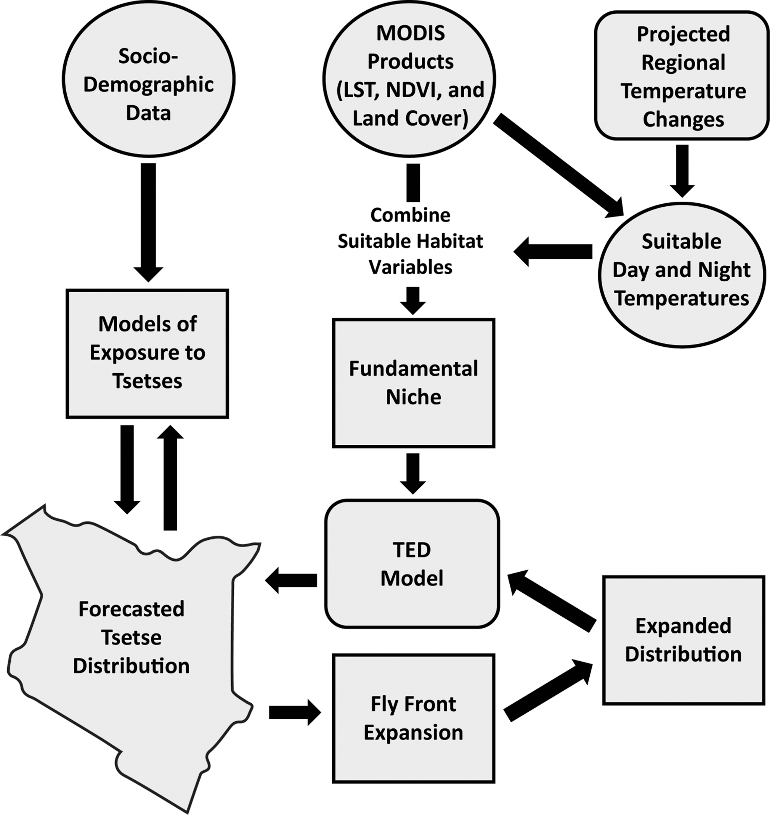
The African Trypanosomiasis Forecasting System (ATcast) modeling outline. Incorporated in this modeling framework is the Tsetse Ecological Distribution (TED) Model, which accounts for spatio-temporal dispersal dynamics of tsetse fly distributions, among various other climatic and nonclimatic factors. Projected regional temperature changes are calculated using the Regional Atmospheric Modeling System (RAMS). MODIS, Moderate Resolution Imaging Spectroradiometer; LST, land surface temperature; NDVI, Normalized Difference Vegetation Index. (Adapted from Messina et al. 2012.)

Many of the studies we reviewed claimed insufficient data for validation (e.g., Martens et al. 1999, Levine et al. 2004, Estrada-Pena and Venzal 2007, Gonzalez et al. 2010, Tonnang et al. 2010, Messina et al. 2012). While mechanistic modeling of disease vectors is one way to counter this problem, independent occurrence data are still needed to validate the models. Paleoecological observations have value for model validation for some species (Martinez-Meyer and Peterson 2006, Willis and Birks 2006, Roberts and Hamann 2012), but their potential for arthropod vectors is limited because some specimens are rarely preserved and because environmental conditions at the time of their preservation can be too uncertain to provide insight into present-day environmental dependence (Borkent and Grimaldi 2004). This also reveals the added challenge of modeling most emerging vector species (e.g., mosquitoes carrying West Nile virus; e.g., Yoo 2014), especially with the historical calibration approach: Historical records will be largely lacking for places of concern. For these cases, historical calibration might not be possible until sufficient vector records have been collected.

A third validation approach was the comparison of occurrence data of arthropod vectors with the locations of infected reservoir species, and it holds significant promise (Table 1). For example, models of phlebotomine sand flies were validated using disease case data on leishmaniasis, for which dogs are a reservoir (Galvez et al. 2011). Leishmaniasis case data were collected from veterinary clinics scattered across 32 villages in Madrid. The number of dogs infected with leishmaniasis, and the locations of the clinic in which they were diagnosed, were recorded. Their locations were then geocoded into a map layer and compared with the map of phlebotomine sand fly vectors and disease presence and predicted phlebotomine distributions were found to be strongly related.

Although the presence of a disease suggests the nearby presence of the vector that transmits it, such as leishmaniasis in dogs carried by the phlebotomine fly, areas where the disease is detectable are commonly subsets of a vector's geographical distributions (Kulkarni et al. 2010). Furthermore, disease cases may be aggregated around the health centers where they were diagnosed and recorded, offering biased measurements of the geographical distribution of disease incidence and, consequently, vector distributions. For example, the human African trypanosomiasis (HAT) vector G. morsitans still inhabits many regions of Tanzania, but HAT is now mainly found in the western and northern regions of the country (Matemba et al. 2010, Malele 2011).

Projecting vector distributions into the future

Studies we reviewed projected future changes in disease vector distributions by substituting future environmental changes into their current spatial models in one of three ways—using GCMs, adding a constant increment of environmental change uniformly throughout the region of interest, or extrapolating recent environmental trends linearly into the future (see Table 1). First, 24 of the 29 papers we reviewed used GCMs to model climate on the basis of its underlying physical processes and used these models to predict geographical variation in future climates under different emissions scenarios. For instance, Lyme disease risk in North America was predicted by modeling Ixodes scapularis tick distributions with current climate data and tick occurrence records and then projecting the current spatial model to 2020, 2050, and 2080 using GCMs in combination with emissions scenarios (Brownstein et al. 2005). While GCMs are believed to remain the most advanced tools available for future projections of climate change (Randall et al. 2007), their outputs still fail to address changes in biological processes through time when the GCMs are projected from only one spatial model.

Second, the use of constant environmental increments set by the study, such as the input of 2°C, 0.1°C, or 4°C increases in temperature combined with 10% increases or decreases in seasonal rainfall across Africa to predict future Anopheles mosquito distributions (Tonnang et al. 2010), assumes that the spatial environmental patterns will remain constant through the modeled period. Retaining constant spatial trends in environmental factors using this approach will lead to discontinuities in predicted vector distributions if modeled environmental differences exceed thresholds of tolerance among vector species in some areas. For this reason, detailed knowledge of the vector's ecology is imperative to these modeling approaches. Information on temperature thresholds for survival is gathered through field observations, such as for the Asian tiger mosquito, Aedes albopictus (Fischer et al. 2014). Upper and lower critical temperatures can also be tested in laboratory settings and then incorporated in future climate scenarios. However, results for survival thresholds can vary substantially between field and laboratory conditions. Because ecological complexity, such as short-term temperature fluctuations, can affect results of survival thresholds in the field, both field and laboratory results should be taken into account when modeling geographic limitations (e.g., Brady et al. 2013). While such measurements are likely to correlate with species' realized thermal niche limits beyond laboratory confines, species' capacities for behavioral thermoregulation are variables among species and among environments (Sunday et al. 2014).

Third, extrapolating from recent environmental trends by adding a constant change increment (e.g., +1°C) is an improvement to setting theoretical increments because its future projections are grounded on observed trends through time. For example, change in irrigated cropland in Sudan and Upper Egypt was first calculated between 2001 and 2009 and then extrapolated to 2050 to predict future Anopheles arabiensis mosquito distributions (Fuller et al. 2012b). However, this method assumes these trends will only continue linearly.

Determining which projection method is most realistic will remain uncertain because the future is uncertain, but ensemble forecasting is a promising solution to increasing forecast robustness (Araujo and New 2007). Multiple model outputs are analyzed for their range of projections. Forecast models derived from different future scenarios are combined using consensus methods to produce outputs and are predicted to be more accurate than forecasts from single models (Forester et al. 2013). Ensemble forecasts can and are already being used in epidemiological forecast models. For instance, projections of Ae. albopictus in Europe used 10 regional climate models and achieved climate projections consistent with the Intergovernmental Panel on Climate Change (IPCC) projections and future hot spots consistent with other published studies (Caminade et al. 2012). But regardless of the method used to project future environmental change, a forecast model will lack credibility unless the magnitude of species' temporal response to environmental change can be approximated.

Each of the projection modeling frameworks we reviewed requires the space-for-time assumption (Pearson et al. 2006, Fisher et al. 2010). That is, observed spatial environmental gradients within the species' current range are assumed to be identical to how it would respond to the temporal environmental changes of similar magnitude. Models are then extrapolated to spatial and temporal domains different from those in which the models were trained (Dobrowski et al. 2011, Kerr et al. 2011). However, spatially accurate models may not be temporally transferrable. Slight differences in the current distributions of species predicted by different models become magnified when those distributions are then projected into future climate scenarios, resulting in a variety of predicted range sizes for the same species and region and increasing projection uncertainty (Kharouba et al. 2009).

If species distributions are at or near equilibrium with environmental conditions (i.e., the current areas where the population is found represent the full possible extent of the population's distribution), it is more likely that models will correctly predict their distributions through time (Botkin et al. 2007, Broennimann and Guisan 2008, Elith and Leathwick 2009, Araujo and Peterson 2012, Pagel and Schurr 2012, Sax et al. 2013, Wenger et al. 2013). Yet, disease vectors are often likened to invasive species in their ability to spread rapidly into new environments through human transport and changes in land use and climate, and equilibrium assumptions are likely to be unreliable (Crowl et al. 2008, Fuller et al. 2012b). The equilibrium assumption may mislead predictions over broad areas, depending on species' traits (e.g., dispersal), so species' capacities to colonize previously unoccupied areas may affect reliability of model predictions (Araujo and Pearson 2005, Leroux et al. 2013).

Understanding dispersal limitations can be crucial. For example, correlative modeling of the potential spread of Ae. albopictus to higher altitudes in the Alps was assessed by relating presences and absences of the mosquito to high-resolution (200-meter) land surface temperature data (Roiz et al. 2011). A temperature gradient–based model was created to fill the no-data areas and, combined with threshold conditions governing egg and adult overwintering survival, the models agreed with previous studies' results of annual and January mean temperature as the most crucial to mosquito dispersal. The authors did not discuss their validation method but do admit that model validation with empirical observations is needed and that they will validate with independent field data as they conduct new vector collections in the coming years. Mechanistic modeling of G. morsitans tsetse flies in Kenya, for example, considers both environmental factors and fly dispersal abilities (Messina et al. 2012). The modeling framework accounts for fly dispersal by setting a “fly front” (i.e., tsetse population movement as a whole, instead of individual tsetse movement rates), where interactions between tsetse distributions and predicted environmentally suitable areas would be considered tsetse presence. The end result consists of 250-meter spatial and 16-day temporal resolution presence–absence tsetse maps (see Fig. 1), validated with tsetse habitat suitability maps from other sources. A cost analysis estimates that if such a predictive modeling system is implemented it will, over an 8-year tsetse management campaign, save Kenya's control programs over $19 million or approximately 58% of normal tsetse control expenditures (McCord et al. 2012).

Historical calibration

A validation method in macroecology that relies on historical calibration of model predictions (Kharouba et al. 2009) is achieving general acceptance in conservation and global change research (Rapacciuolo et al. 2014; described in Fig. 2). We found no studies that have yet used this framework for predicting changing vector distributions through time, so we describe its utility by drawing on examples from macroecological and global change research. The key benefit of this framework is to evaluate the reliability of the space-for-time assumption and provide a direct test of whether spatial models are temporally transferrable in the context of a natural, or pseudo-, experiment (Kerr et al. 2007).

FIG. 2.

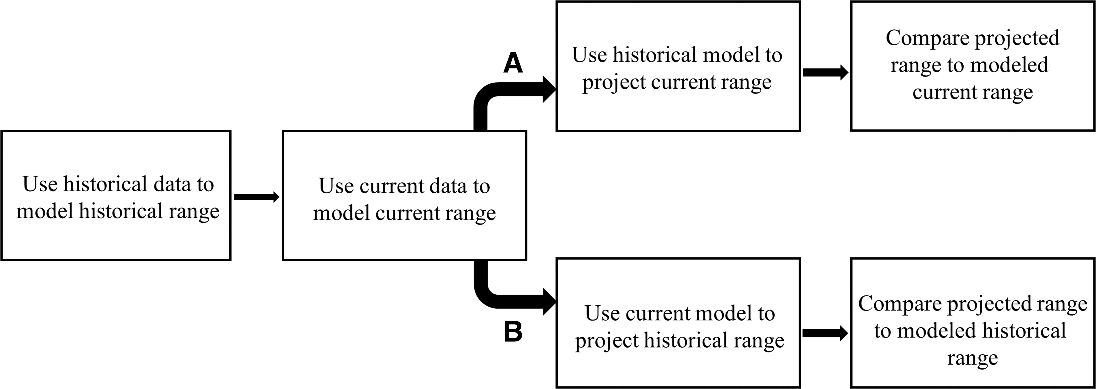
Methodology applied when using historical species occurrence data to validate species niche models through time (adapted from Kharouba et al. 2009), where models can be forecasted (A), hindcasted (B), or both.

Historically calibrated distribution models employ the usual tests of model fit, based on cross-validation and statistical accuracy assessment (e.g., AUC and TSS). However, predictions of how a species' distribution will change through time are tested through a period during which such changes can be observed directly. For example, butterfly distributions across Canada were examined in a historical period (1900–1930; Kharouba et al. 2009). Each of these species' range responses to subsequent climate change was tested by substituting observed climate measures from 1960 to 1990 into this historical model and predicting how their ranges should have changed if historical relationships between climate and species' occurrences remained constant. Predictions for the latter time period (1960–1990) could then be tested in two ways. The first involves recalculating model accuracy statistics based on new occurrence points from that latter time period. The second involves constructing new models from latter observations for comparison with historical model predictions. Predictions of butterfly species distribution changes over the 20th century across Canada were strongly correlated with observed changes in those distributions. These studies assume that species do not adapt to novel environmental conditions through the observed or anticipated time periods. While that assumption appeared reasonable for butterflies in Canada, which often have one generation per year, uncertainties regarding disease vectors' potential to adapt to new environments (particularly since many breed extremely rapidly in far less seasonal environments than Canada) are substantial (Fischer et al. 2014).

The use of multitemporal species observations and environmental data reduces the uncertainty imposed by the space-for-time assumption. Minimally, using historical data to test (or validate) model predictions through time will reveal clear violations of the assumption, such as instances when models appear spatially accurate but predict nonsensically through time (e.g., Pearson et al. 2006). Yet, predicting future conditions will always require this assumption: Changes observed recently will continue to reflect changes anticipated through the future period that is being modeled. Both forecasting (Fig. 2A) and backcasting (or hindcasting; Fig. 2B) can provide some measure of historical calibration for model predictions. These historical calibration methods are finding increased application, especially in conjunction with advancing measures of species' dispersal capacities, population growth, and even species' particular behavioral thermoregulatory strategies under continuously varying environmental changes (e.g., Monahan and Tingley 2012, Sunday et al. 2012, Leroux et al. 2013, Sunday et al. 2014). Opportunities to use this framework to gain biological insights into vector responses to global change appear substantial, particularly given the increasing availability of historical species observations.

Advanced modeling techniques, rapidly evolving satellite remote-sensing tools, and increased vector surveillance provide the tools necessary for building historically calibrated vector models. For instance, forecast models of Anopheles mosquitoes are advancing with both mechanistic (e.g., Yamana and Eltahir 2013) and correlative (e.g., Tonnang et al. 2010) approaches at macroscales. Satellite-borne remote-sensing data sources, such as the Moderate Resolution Imaging Spectroradiometer (MODIS; https://lpdaac.usgs.gov/products/modis_products_table/modis_overview) are increasingly accessible and provide high resolution (up to 250 meters for MODIS), near-real time measurements of both climate and land use changes over very broad areas (see Fig. 3). Occurrence records for vectors, like Anopheles mosquitoes, are also increasingly accessible through online sources, such as the Global Biodiversity Information Facility (www.gbif.org), Malaria Atlas Project (www.map.ox.ac.uk), and IRMapper (www.irmapper.com), and primary research publications also provide large assemblages of these observations. Nevertheless, occurrence records for many species remain difficult to find (noted in several studies here: Estrada-Pena and Venzal 2007, Gonzalez et al. 2010, Messina et al. 2012), and predicting changes in associated disease risk will remain proportionately more difficult (and interventions harder to implement) while this problem persists.

FIG. 3.

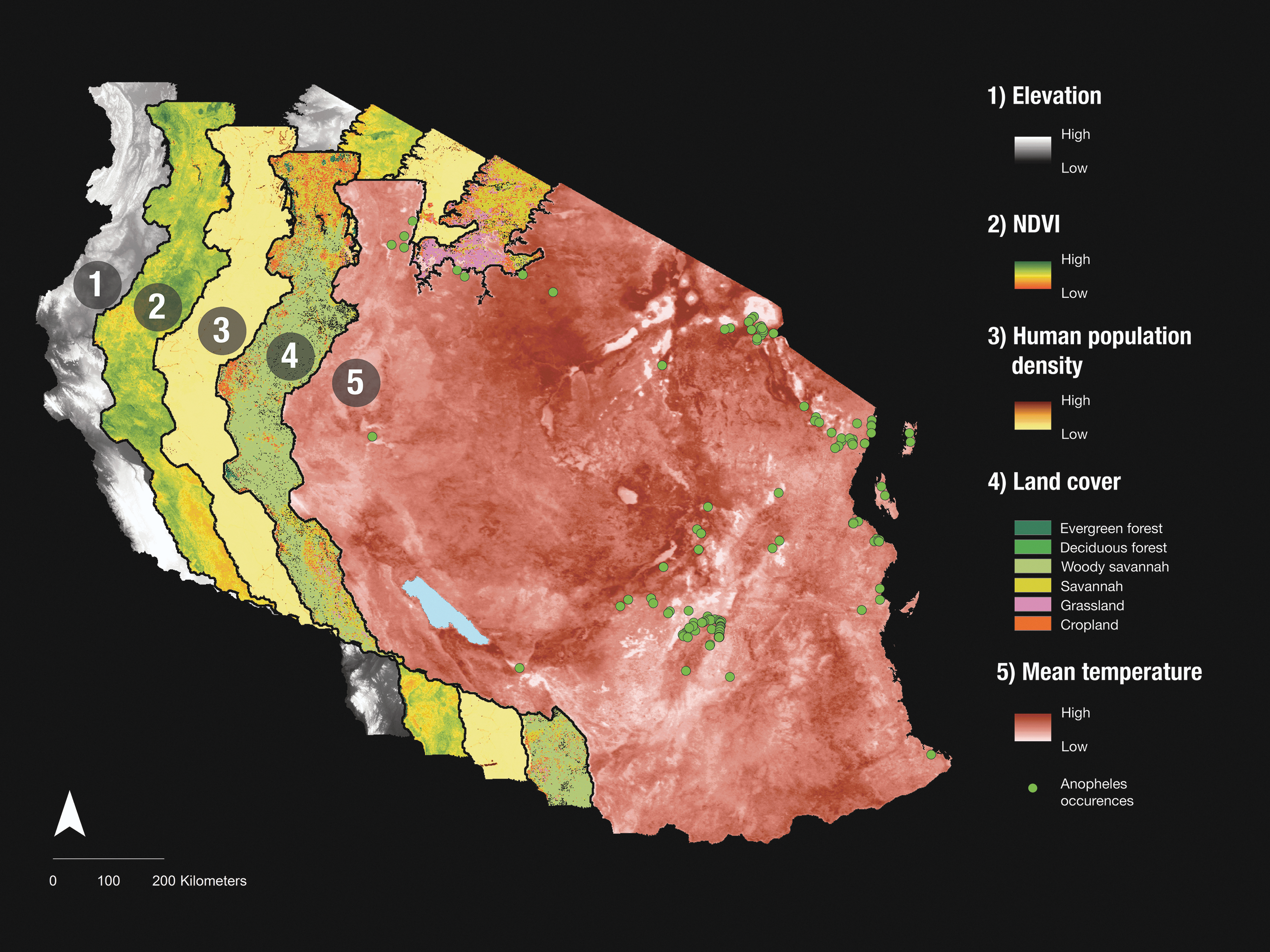
Different satellite imagery layers for mainland Tanzania in 2001 from the Shuttle Radar Topography Mission (SRTM, elevation) and Moderate Resolution Imaging Spectroradiometer (MODIS) used in conjunction with Anopheles mosquito occurrence records for predictive modeling. These satellite data can often be acquired for multiple years and even in areas where environmental data sampling is sparse.

Although historical calibration of species distribution models does not eliminate shortcomings intrinsic to predicting an uncertain future, it reduces or resolves more challenges than it creates. This historical calibration and testing framework reduces the risk that spatial autocorrelation may create misleading fits between environmental predictors and species distributions, but it cannot eliminate potential impacts of autocorrelation, which exists temporally as well as spatially. Yet, a key benefit is a direct test of the temporal transferability of a species distribution model that might otherwise provide only a snapshot of a species' reliance on environmental conditions over broad areas. When accompanied by more reliable projection methods, like ensemble forecasting, historically calibrated forecast models increasingly address the current dilemma of determining predictive model accuracy over areas where vector range changes have actually been tracked through time.

Conclusions

Validation through historical calibration is increasingly used for macroecological and global change research and could be adapted readily for epidemiological models forecasting disease vector distributions. Tests of model transferability, used with other statistical tests of model fit, will increase confidence in model predictions both spatially and temporally. Availability of reliable species observations over broad areas and at different times is a significant impediment here, as it has been for macroecological and global change research. Increased and consistent disease vector occurrence data collections are urgently needed. Forecasting disease vector distributions is further complicated by inadvertent or careless introductions of vectors into new areas (Sutherst 2004, Fischer et al. 2014). For example, chikungunya was recently found in St. Maarten in December of 2013, the first recorded instance of local transmission of the disease in the Western Hemisphere (Centers for Disease Control and Prevention 2014). Despite continuous improvements in techniques that assess how vector species' distributions and abundances depend on environmental conditions, predicting their future distributions will remain a challenging endeavor. Nevertheless, interdisciplinary opportunities to improve biological understanding of how and when vector species will respond to environmental changes could improve prospects for successful interventions to reduce their impacts on human health. Historical validation is one such opportunity.

Footnotes

Acknowledgments

We thank Andrew Plowright, Alana Taylor-Pindar, Laura Coristine, and the two anonymous reviewers for their helpful edits with the manuscript. E.S.A. acknowledges the Natural Sciences and Engineering Research Council of Canada (NSERC) for support, and J.T.K. is grateful for NSERC Discovery Grant support and to the University Research Chairs program at the University of Ottawa.

Author Disclosure Statement

No competing financial interests exist.

References

Acevedo

, Ruiz-Fons

, Estrada

, Marquez

, et al. A broad assessment of factors determining Culicoides imicola abundance: Modelling the present and forecasting its future in climate change scenarios. Plos One, 2010; 5:e14236.

Algar

, Kharouba

, Young

, Kerr

. Predicting the future of species diversity: Macroecological theory, climate change, and direct tests of alternative forecasting methods. Ecography, 2009; 32:22–33.

Allouche

, Tsoar

, Kadmon

. Assessing the accuracy of species distribution models: Prevalence, kappa and the true skill statistic (TSS). J Appl Ecol, 2006; 43:1223–1232.

Araujo

, Guisan

. Five (or so) challenges for species distribution modelling. J Biogeogr, 2006; 33:1677–1688.

Araujo

, New

. Ensemble forecasting of species distributions. Trends Ecol Evol, 2007; 22:42–47.

Araujo

, Pearson

. Equilibrium of species' distributions with climate. Ecography, 2005; 28:693–695.

Araujo

, Peterson

. Uses and misuses of bioclimatic envelope modeling. Ecology, 2012; 93:1527–1539.

Araujo

, Pearson

, Thuiller

, Erhard

. Validation of species-climate impact models under climate change. Global Change Biol, 2005a; 11:1504–1513.

Araujo

, Whittaker

, Ladle

, Erhard

. Reducing uncertainty in projections of extinction risk from climate change. Global Ecol Biogeogr, 2005b; 14:529–538.

10.

Bahn

, McGill

. Testing the predictive performance of distribution models. Oikos, 2013; 122:321–331.

11.

Beebe

, Cooper

, Mottram

, Sweeney

. Australia's dengue risk driven by human adaptation to climate change. Plos Negl Trop Dis, 2009; 3:9.

12.

Blois

, Williams

, Fitzpatrick

, Jackson

, et al. Space can substitute for time in predicting climate-change effects on biodiversity. Proc Natl Acad Sci USA, 2013; 110:9374–9379.

13.

Borkent

, Grimaldi

. The earliest fossil mosquito (Diptera: Culicidae), in mid-Cretaceous Burmese amber. Ann Entomol Soc Am, 2004; 97:882–888.

14.

Botkin

, Saxe

, Araujo

, Betts

, et al. Forecasting the effects of global warming on biodiversity. Bioscience, 2007; 57:227–236.

15.

Brady

, Johansson

, Guerra

, Bhatt

, et al. Modelling adult Aedes aegypti and Aedes albopictus survival at different temperatures in laboratory and field settings. Parasites Vectors, 2013; 6:351.

16.

Braunisch

, Coppes

, Arlettaz

, Suchant

, et al. Selecting from correlated climate variables: A major source of uncertainty for predicting species distributions under climate change. Ecography, 2013; 36:971–983.

17.

Broennimann

, Guisan

. Predicting current and future biological invasions: Both native and invaded ranges matter. Biol Lett, 2008; 4:585–589.

18.

Brown

, Maurer

. Macroecology—The division of food and space among species on continents. Science, 1989; 243:1145–1150.

19.

Brownstein

, Holford

, Fish

. Effect of climate change on Lyme disease risk in North America. EcoHealth, 2005; 2:38–46.

20.

Caminade

, Medlock

, Ducheyne

, McIntyre

, et al. Suitability of European climate for the Asian tiger mosquito Aedes albopictus: Recent trends and future scenarios. J R Soc Interface, 2012; 9:2708–2717.

21.

Centers for Disease Control and Prevention. Chikungunya in the Caribbean. CDC: Centers for Disease Control and Prevention, 2014.

22.

Cross

, Hyams

. The potential effect of global warming on the geographic and seasonal distribution of Phlebotomus papatasi in Southwest Asia. Environ Health Perspect, 1996; 104:724–727.

23.

Crowl

, Crist

, Parmenter

, Belovsky

, et al. The spread of invasive species and infectious disease as drivers of ecosystem change. Front Ecol Environ, 2008; 6:238–246.

24.

DeVisser

, Messina

, Moore

, Lusch

, et al. A dynamic species distribution model of Glossina subgenus Morsitans: The identification of tsetse reservoirs and refugia. Ecosphere. Ecosphere: Ecological Society of America, 2010.

25.

Dobrowski

, Thorne

, Greenberg

, Safford

, et al. Modeling plant ranges over 75 years of climate change in California, USA: Temporal transferability and species traits. Ecol Monogr, 2011; 81:241–257.

26.

Dormann

. Promising the future? Global change projections of species distributions. Basic Appl Ecol, 2007; 8:387–397.

27.

Drake

, Beier

. Ecological niche and potential distribution of Anopheles arabiensis in Africa in 2050. Malaria J, 2014; 13:213.

28.

Duncombe

, Clements

, Davis

, Hu

, et al. Spatiotemporal patterns of Aedes aegypti populations in Cairns, Australia: Assessing drivers of dengue transmission. Trop Med Int Health, 2013; 18:839–849.

29.

Elith

, Leathwick

. Species distribution models: Ecological explanation and prediction across space and time. Ann Rev Ecol Evol Systematics, 2009: 40:677–697.

30.

Erickson

, Hayhoe

, Presley

, Allen

LJS

, et al. Potential impacts of climate change on the ecology of dengue and its mosquito vector the Asian tiger mosquito (Aedes albopictus). Environ Res Lett, 2012; 7:6.

31.

Estrada-Pena

, Venzal

. Climate niches of tick species in the Mediterranean region: Modeling of occurrence data, distributional constraints, and impact of climate change. J Med Entomol, 2007; 44:1130–1138.

32.

Feria-Arroyo

, Castro-Arellano

, Gordilo-Perez

, Cavazos

, et al. Implications of climate change on the distribution of the tick vector Ixodes scapularis and risk for Lyme disease in the Texas-Mexico transboundary region. Parasit Vectors, 2014; 7:199.

33.

Fielding

, Haworth

. Testing the generality of bird-habitat models. Conserv Biol, 1995; 9:1466–1481.

34.

Fischer

, Thomas

, Niemitz

, Reineking

, et al. Projection of climatic suitability for Aedes albopictus Skuse (Culicidae) in Europe under climate change conditions. Global Planet Change, 2011; 78:54–64.

35.

Fischer

, Thomas

, Neteler

, Tjaden

, et al. Climatic suitability of Aedes albopictus in Europe referring to climate change projections: Comparison of mechanistic and correlative niche modelling approaches. Eurosurveillance, 2014; 19:34–46.

36.

Fisher

JAD

, Frank

, Leggett

. Dynamic macroecology on ecological time-scales. Global Ecol Biogeogr, 2010; 19:1–15.

37.

Forester

, DeChaine

, Bunn

. Integrating ensemble species distribution modelling and statistical phylogeography to inform projections of climate change impacts on species distributions. Divers Distrib, 2013; 19:1480–1495.

38.

Fuller

, Ahumada

, Quinones

, Herrera

, et al. Near-present and future distribution of Anopheles albimanus in Mesoamerica and the Caribbean Basin modeled with climate and topographic data. Int J Health Geo, 2012a; 11:12.

39.

Fuller

, Parenti

, Hassan

, Beier

. Linking land cover and species distribution models to project potential ranges of malaria vectors: An example using Anopheles arabiensis in Sudan and Upper Egypt. Malaria J, 2012b; 11:11.

40.

Galvez

, Descalzo

, Guerrero

, Miro

, et al. Mapping the current distribution and predicted spread of the leishmaniasis sand fly vector in the Madrid eegion (Spain) based on environmental variables and expected climate change. Vector Borne Zoonotic Dis, 2011; 11:799–806.

41.

Garza

, Feria Arroyo

, Casillas

, Sanchez-Cordero

, et al. Projected future distributions of vectors of Trypanosoma cruzi in North America under climate change scenarios. PLoS Negl Trop Dis, 2014; 8:e2818.

42.

Gonzalez

, Wang

, Strutz

, Gonzalez-Salazar

, et al. Climate change and risk of leishmaniasis in North America: Predictions from ecological niche models of vector and reservoir species. Plos Negl Trop Dis, 2010; 4:16.

43.

Gonzalez

, Paz

, Ferro

. Predicted altitudinal shifts and reduced spatial distribution of Leishmania infantum vector species under climate change scenarios in Colombia. Acta Trop, 2014; 129:83–90.

44.

Guichard

, Guis

HLN

, Tran

, Garros

, et al. Worldwide niche and future potential distribution of Culicoides imicola, a major vector of bluetongue and African horse sickness virus. PloS One, 2014; 9:e112491.

45.

Hay

, Randolph

, Rogers

. Remote Sensing and Geographical Information Systems in Epidemiology. Elsevier, 2000; 47:1–367.

46.

Hongoh

, Berrang-Ford

, Scott

, Lindsay

. Expanding geographical distribution of the mosquito, Culex pipiens, in Canada under climate change. Appl Geogr, 2012; 33:53–62.

47.

Kearney

, Porter

. Mechanistic niche modelling: Combining physiological and spatial data to predict species' ranges. Ecol Lett, 2009; 12:334–350.

48.

Keith

, Webb

, Bohning-Gaese

, Connolly

, et al. What is macroecology?. Biol Lett, 2012; 8:904–906.

49.

Kerr

, Ostrovsky

. From space to species: Ecological applications for remote sensing. Trends Ecol Evol, 2003; 18:299–305.

50.

Kerr

, Kharouba

, Currie

. The macroecological contribution to global change solutions. Science, 2007; 316:1581–1584.

51.

Kerr

, Kulkarni

, Algar

. Integrating theory and predictive modeling for conservation research. In: Drew

, Wiersma

, Huettmann

, eds. Predictive Species and Habitat Modeling in Landscape Ecology. New York: Springer, 2011:9–28.

52.

Kharouba

, Algar

, Kerr

. Historically calibrated predictions of butterfly species' range shift using global change as a pseudo-experiment. Ecology, 2009; 90:2213–2222.

53.

Kitron

. Landscape ecology and epidemiology of vector-borne diseases: Tools for spatial analysis. J Med Entomol, 1998; 35:435–445.

54.

Kolivras

. Changes in dengue risk potential in Hawaii, USA, due to climate variability and change. Clim Res, 2010; 42:1–11.

55.

Kulkarni

, Desrochers

, Kerr

. High resolution niche models of malaria vectors in northern Tanzania: A new capacity to predict malaria risk?. PloS One, 2010; 5:e9396.

56.

Legendre

, Legendre

LFJ

. Numerical Ecology. Amsterdam: Elsevier Science, 1998.

57.

Leroux

, Larrivee

, Boucher-Lalonde

, Hurford

, et al. Mechanistic models for the spatial spread of species under climate change. Ecol Appl, 2013; 23:815–828.

58.

Levine

, Peterson

, Benedict

. Geographic and ecologic distributions of the Anopheles gambiae complex predicted using a genetic algorithm. Am J Trop Med Hyg, 2004; 70:105–109.

59.

Lobo

, Jimenez-Valverde

, Real

. AUC: A misleading measure of the performance of predictive distribution models. Global Ecol Biogeogr, 2008; 17:145–151.

60.

Malele

. Fifty years of tsetse control in Tanzania: Challenges and prospects for the future. Tanzania J Health Res, 2011; 13.

61.

Martens

, Kovats

, Nijhof

, de Vries

, et al. Climate change and future populations at risk of malaria. Global Environ Change, 1999; 9:S89–S107.

62.

Martinez-Meyer

, Peterson

. Conservatism of ecological niche characteristics in North American plant species over the Pleistocene-to-Recent transition. J Biogeogr, 2006; 33:1779–1789.

63.

Matemba

, Fevre

, Kibona

, Picozzi

, et al. Quantifying the burden of Rhodesiense sleeping sickness in Urambo District, Tanzania. PloS Negl Trop Dis, 2010; 4:10.

64.

McCord

, Messina

, Campbell

, Grady

. Tsetse fly control in Kenya's spatially and temporally dynamic control reservoirs: A cost analysis. Appl Geogr, 2012; 34:189–204.

65.

Meade

, Earickson

. Medical Geography. New York: Guilford Press, 2000:501.

66.

Medlock

, Avenell

, Barrass

, Leach

. Analysis of the potential for survival and seasonal activity of Aedes albopictus (Diptera: Culicidae) in the United Kingdom. J Vector Ecol, 2006; 31:292–304.

67.

Messina

, Moore

, DeVisser

, McCord

, et al. Climate change and risk projection: Dynamic spatial models of tsetse and African trypanosomiasis in Kenya. Ann Assoc of Am Geographers, 2012; 102:1038–1048.

68.

Mills

, Gage

, Khan

. Potential influence of climate change on vector-borne and zoonotic diseases: A review and proposed research plan. Environ Health Perspect, 2010; 118:1507–1514.

69.

Monahan

, Tingley

. Niche tracking and rapid establishment of distributional equilibrium in the house sparrow show potential responsiveness of species to climate change. PloS One, 2012; 7:e42097.

70.

Moo-Llanes

, Ibarra-Cerdena

, Rebollar-Tellez

, Ibanez-Bernal

, et al. Current and future niche of North and Central American sand flies (Diptera: Psychodidae) in climate change scenarios. PloS Negl Trop Dis, 2013; 7:e2421.

71.

Morin

, Comrie

. Modeled response of the West Nile virus vector Culex quinquefasciatus to changing climate using the dynamic mosquito simulation model. Int J Biometeorol, 2010; 54:517–529.

72.

Naish

, Mengerson

, Hu

, Tong

. Forecasting the future risk of Barmah Forest virus disease under climate change scenarios in Queensland, Australia. PloS One, 2013; 8:e62843.

73.

Ogden

, Maarouf

, Barker

, Bigras-Poulin

, et al. Climate change and the potential for range expansion of the Lyme disease vector Ixodes scapularis in Canada. Int J Parasitol, 2006; 36:63–70.

74.

Ogden

, St-Onge

, Barker

, Brazeau

, et al. Risk maps for range expansion of the Lyme disease vector, Ixodes scapularis, in Canada now and with climate change. Int J Health Geo, 2008; 7:15.

75.

Pagel

, Schurr

. Forecasting species ranges by statistical estimation of ecological niches and spatial population dynamics. Global Ecol Biogeogr, 2012; 21:293–304.

76.

Pavlovsky

. Natural Nidality of Transmissible Diseases: With Species Reference to the Landscape Epidemiology of Zooanthroponoses. Champaign, IL: University of Illinois Press, 1966.

77.

Pearson

, Thuiller

, Araujo

, Martinez-Meyer

, et al. Model-based uncertainty in species range prediction. J Biogeogr, 2006; 33:1704–1711.

78.

Peterson

. Ecologic niche modeling and spatial patterns of disease transmission. Emerg Infect Dis, 2006; 12:1822–1826.

79.

Peterson

, Shaw

. Lutzomyia vectors for cutaneous leishmaniasis in Southern Brazil: Ecological niche models, predicted geographic distributions, and climate change effects. Int J Parasitol, 2003; 33:919–931.

80.

Phillips

, Anderson

, Schapire

. Maximum entropy modeling of species geographic distributions. Ecol Model, 2006; 190:231–259.

81.

Randall

, Wood

, Bony

, Colman

, et al. Climate Change 2007: The Physical Science Basis. Contribution of Working Group I to the Fourth Assessment Report of the Intergovernmental Panel on Climate Change. Climate Models and Their Evaluation. United Kingdom: Cambridge University Press, 2007:589–662.

82.

Randin

, Dirnboeck

, Dullinger

, Zimmermann

, et al. Are niche-based species distribution models transferable in space?. J Biogeogr, 2006; 33:1689–1703.

83.

Rapacciuolo

, Roy

, Gillings

, Purvis

. Temporal validation plots: Quantifying how well correlative species distribution models predict species' range changes over time. Methods Ecol Evol, 2014; 5:407–420.

84.

Rastetter

. Validating models of ecosystem response to global change. Bioscience, 1996; 46:190–198.

85.

Reisen

. Landscape epidemiology of vector-borne diseases. Annu Rev Entomol, 2010; 55:461–483.

86.

Roberts

, Hamann

. Method selection for species distribution modelling: are temporally or spatially independent evaluations necessary?. Ecography, 2012; 35:792–802.

87.

Roiz

, Neteler

, Castellani

, Arnoldi

, et al. Climatic factors driving invasion of the tiger mosquito (Aedes albopictus) into new areas of Trentino, northern Italy. PloS One, 2011; 6:e14800.

88.

Sax

, Early

, Bellemare

. Niche syndromes, species extinction risks, and management under climate change. Trends Ecol Evol, 2013; 28:517–523.

89.

Schafer

, Lundstrom

. The present distribution and predicted geographic expansion of the floodwater mosquito Aedes sticticus in Sweden. J Vector Ecol, 2009; 34:141–147.

90.

Sobek-Swant

, Kluza

, Cuddington

, Lyons

. Potential distribution of emerald ash borer: What can we learn from ecological niche models using Maxent and GARP?. For Ecol Manage, 2012; 281:23–31.

91.

Stockwell

, Peters

. The GARP modelling system: Problems and solutions to automated spatial prediction. Int J Geogr Information Sci, 1999; 13:143–158.

92.

Sunday

, Bates

, Dulvy

. Thermal tolerance and the global redistribution of animals. Nature Climate Change, 2012; 2:686–690.

93.

Sunday

, Bates

, Kearney

, Colwell

, et al. Thermal-safety margins and the necessity of thermoregulatory behavior across latitude and elevation. Proc Natl Acad Sci USA, 2014; 111:5610–5615.

94.

Sutherst

. Global change and human vulnerability to vector-borne diseases. Clin Microbiol Rev, 2004; 17:136–173.

95.

Tabachnick

. Challenges in predicting climate and environmental effects on vector-borne disease episystems in a changing world. J Exp Biol, 2010; 213:946–954.

96.

Thuiller

. BIOMOD—optimizing predictions of species distributions and projecting potential future shifts under global change. Global Change Biol, 2003; 9:1353–1362.

97.

Tonnang

HEZ

, Kangalawe

RYM

, Yanda

. Predicting and mapping malaria under climate change scenarios: The potential redistribution of malaria vectors in Africa. Malaria J, 2010; 9:111.

98.

Trejo

, Martinez-Meyer

, Calixto-Perez

, Sanchez-Colon

, et al. Analysis of the effects of climate change on plant communities and mammals in Mexico. Atmosfera, 2011; 24:1–14.

99.

Ureta

, Martinez-Meyer

, Perales

, Alvarez-Buylla

. Projecting the effects of climate change on the distribution of maize races and their wild relatives in Mexico. Global Change Biol, 2012; 18:1073–1082.

100.

Wenger

, Som

, Dauwalter

, Isaak

, et al. Probabilistic accounting of uncertainty in forecasts of species distributions under climate change. Global Change Biol, 2013; 19:3343–3354.

101.

White

, Kerr

. Contrasting spatial and temporal global change impacts on butterfly species richness during the 20th century. Ecography, 2006; 29:908–918.

102.

Willis

, Birks

HJB

. What is natural? The need for a long-term perspective in biodiversity conservation. Science, 2006; 314:1261–1265.

103.

World Health Organization. World Health Report 2008.. 2008:1–190.

104.

Yamana

, Eltahir

EAB

. Projected impacts of climate change on environmental suitability for malaria transmission in West Africa. Environ Health Perspect, 2013; 121:1179–1186.

105.

Yoo

. Site-specific prediction of West Nile virus mosquito abundance in Greater Toronto Area using generalized linear mixed models. Int J Geogr Information Sci, 2014; 28:296–313.