Two Introductions of Lyme Disease into Connecticut: A Geospatial Analysis of Human Cases from 1984 to 2012

Abstract

Lyme disease has become the most prevalent vector-borne disease in the United States and results in morbidity in humans, especially children. We used historical case distributions to explain vector-borne disease introductions and subsequent geographic expansion in the absence of disease vector data. We used geographic information system analysis of publicly available Connecticut Department of Public Health case data from 1984, 1985, and 1991 to 2012 for the 169 towns in Connecticut to identify the yearly clusters of Lyme disease cases. Our analysis identified the spatial and temporal origins of two separate introductions of Lyme disease into Connecticut and identified the subsequent direction and rate of spread. We defined both epidemic clusters of cases using significant long-term spatial autocorrelation. The incidence-weighted geographic mean analysis indicates a northern trend of geographic expansion for both epidemic clusters. In eastern Connecticut, as the epidemic progressed, the yearly shift in the geographic mean (rate of epidemic expansion) decreased each year until spatial equilibrium was reached in 2007. The equilibrium indicates a transition from epidemic Lyme disease spread to stable endemic transmission, and we associate this with a reduction in incidence. In western Connecticut, the parabolic distribution of the yearly geographic mean indicates that following the establishment of Lyme disease (1988) the epidemic quickly expanded northward and established equilibrium in 2009.

Introduction

Lyme disease was first identified in 1975 when researchers investigated a cluster of juvenile arthritis cases in close proximity to the coastal town of Lyme, Connecticut (Steere et al. 1978, Steere 1997). Symptoms included a distinctive bull's-eye rash (erythema migrans), flu-like symptoms (fatigue, headaches, joint and muscle pain, and fever), and, if untreated, neurologic, cardiac, or articular complications (Steere et al. 1977, 1979). In North America, Lyme disease results from infection by the spirochete bacterium Borrelia burgdorferi and is transmitted throughout the eastern United States by the black-legged tick Ixodes scapularis (Lastavica et al. 1989, Stafford et al. 1998, Falco et al. 1999). Lyme disease is the most common vector-borne disease in the United States of America and has spread throughout Connecticut. Case distributions within the state are not consistent with a single introduction of the disease in Lyme, Connecticut. Understanding the origins and subsequent spread of Lyme disease is important for predicting risk and future disease spread. These predictions are particularly important in light of global climate change and the increasing number of northern cases in previously uninfected areas.

Typically the use of human case data to track disease progression is inconsistent because of problems associated with sensitivity (misreporting/misdiagnosis of cases), reporting fatigue, changes in case definition, and changes in surveillance techniques. These problems create variation around the true data and may obscure data trends. However, previous studies have shown the value of using human surveillance data to model spatial trends in vector-borne and zoonotic diseases (White et al. 1991, Kitron and Kazmierczak 1997, Glavanakov et al. 2001, Childs et al. 2007). Kitron and Kazmierczak generated a map delineating counties with the highest risk for Lyme disease according to the correlation between tick distribution and human case distribution by county of exposure (Kitron and Kazmierczak 1997). Glavanakov et al. (2001) estimated a regional correlation distance from Lyme disease human incidence reported by New York State counties from 1988 to 1996 using spatial autocorrelation methods. Connecticut has long-term datasets (Petersen et al. 1989) describing Lyme disease case distribution in 1984 and 1985, and the Connecticut Department of Public Health has historical Lyme disease records throughout the state from 1991 to 2012. However, Ertel et al. (2012) detailed potential problems with using the long-term datasets due to changes of surveillance methods.

Eisen et al. (2012) assessed potential reasons for the continued lack of success and control of Lyme disease in the northeastern United States. This study describes the spatial-temporal patterns of Lyme disease from 1984 to 2012 using human case reports in the state of Connecticut with a specific focus on how both eastern and western Connecticut have experienced Lyme disease epidemics (Fig. 1). Two spatially and temporally separate disease introductions are identified. The two epidemics have similar characteristics such as a northern direction of spread, rate of expansion, and trends in normalized incidence after the epidemic wave passes.

FIG. 1.

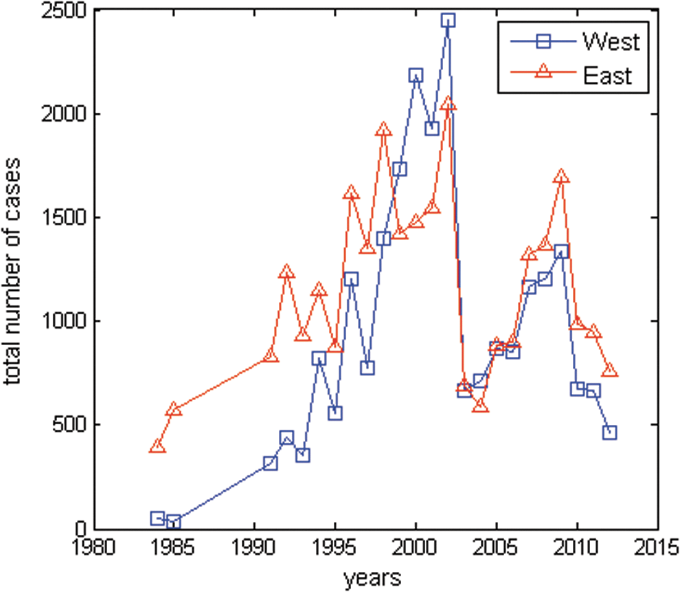
Yearly Lyme disease cases in eastern and western Connecticut. The total number of yearly Lyme disease cases in 91 eastern and 78 western towns in Connecticut for 1984, 1985, and 1991–2012. Yearly fluctuations in total Lyme disease cases are influenced by the reporting method, but the trends in yearly cases remain consistent with high case numbers during the epidemic phase and a transition to lower numbers during the endemic phase.

Materials and Methods

Case report data

Connecticut has conducted active Lyme disease surveillance since 1984; federally mandated reporting started in 1987, when a physician-based surveillance system was established. The surveillance system has undergone changes to improve the reporting quality, especially during 1998–2007 when Lyme disease was added to the list of significant laboratory findings (Ertel et al. 2007). All Lyme disease cases used in this study were selected according to the 1987 case report definition (Centers for Disease Control and Prevention [CDC] 1997). Due to reporting inconsistencies in earlier data, this research only used cases from 1984 and 1985 collected by Peterson et al. (1989) and 1991–2012 from the Connecticut Department of Public Health website (www.ct.gov/dph/cwp/view.asp?a=3136&q=399694). The data are tracking the human cases instead of pathogen or vectors.

Normalized incidence was calculated as the number of Lyme disease cases reported each year divided by the town population and normalized to 10,000 people. Rates were computed each year for all 169 towns in Connecticut, and geographic mean centers were identified according to incidence rates and locations.

Spatial analysis

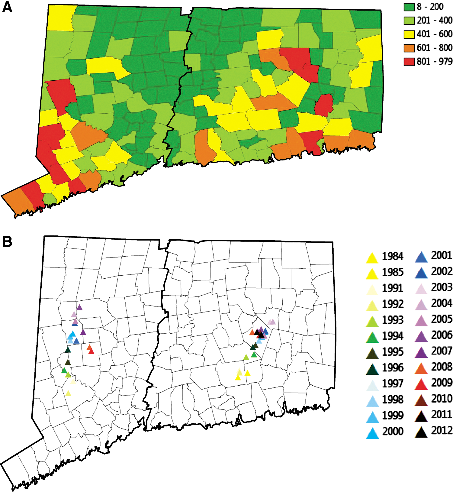
After visualizing the yearly incidence for all the towns in Connecticut using ArcGIS 10 (the 24 yearly maps are not shown), and examining the total cases per town from 1984, 1985, and 1991–2012 (Fig. 2A), two disease clusters or epidemic clusters were apparent. After defining the clustered cases in eastern and western Connecticut, Global Moran's I values (p<0.05, Z>2.90 with Bonferroni correction) were used to test for significant spatial autocorrelation of the cases. Geographic structuring of the yearly cases indicates that townships with similar incidence of Lyme disease are more closely related than townships more distant. Global Moran's I values (Boots and Tiefelasdorf 2000) calculated by MATLAB (2009a) using inverse of distance between towns as weights and incidence rate in each town as data, are shown in Table 1.

FIG. 2.

(A) The total number of cases in Connecticut in 1984, 1985, 1991–2012. Human cases cluster in eastern and western Connecticut with few cases between the two clusters. The greatest number of cases is in the most populated areas, although the geographic distribution of cases and highest incidence is on the northern edge of the expanding epidemic. (B) The yearly incidence-weighted geographic means. The geographic means computed using Equations (1) and (2) for 1984, 1985, and 1991–2012 are represented by colors. Geographic expansion of the Lyme disease clusters is visualized by the distance between and direction of the yearly means. Only the geographic means with significant Global Moran's I values are shown.

Table 1.

Global Moran's I Test for Spatial Autocorrelation or Spatial Structure of Yearly Lyme Disease Cases In Connecticut ^a

	Western		Eastern
Year	Morans I	Z-score	Morans I	Z-score
1984	0.0013	0.9867	0.1064	9.6238
1985	−0.0135	−0.0360	0.0954	8.7286
1991	0.0510	4.4220	0.1226	10.9532
1992	0.1148	8.8212	0.1754	15.2698
1993	0.0621	5.1839	0.1077	9.7258
1994	0.0826	6.5964	0.1024	9.2905
1995	0.0881	6.9762	0.1277	11.3621
1996	0.0969	7.5835	0.1305	11.5888
1997	0.0874	6.9270	0.1142	10.2622
1998	0.0901	7.1137	0.1522	13.3666
1999	0.0738	5.9934	0.1667	14.5529
2000	0.0709	5.7929	0.1816	15.7678
2001	0.0791	6.3582	0.1641	14.3396
2002	0.0699	5.7311	0.2109	18.1712
2003	0.0738	5.9963	0.1932	16.7192
2004	0.0913	7.2048	0.1162	10.4360
2005	0.0941	7.3954	0.1593	13.9412
2006	0.0927	7.3034	0.1711	14.9127
2007	0.1153	8.8523	0.1581	13.8468
2008	0.0424	3.8184	0.1096	9.8815
2009	0.0470	4.1351	0.1603	14.0263
2010	−0.0031	0.6822	0.1342	11.8966
2011	0.0163	2.0208	0.1286	11.4351
2012	−0.0014	0.7971	0.1423	12.5571

Significant (p<0.05, Z<2.90 with Bonferonni correction) Z-distribution values are in italic and boldface for clarity.

The formula for calculating Global Moran's I values is: \documentclass{aastex}\usepackage{amsbsy}\usepackage{amsfonts}\usepackage{amssymb}\usepackage{bm}\usepackage{mathrsfs}\usepackage{pifont}\usepackage{stmaryrd}\usepackage{textcomp}\usepackage{portland, xspace}\usepackage{amsmath, amsxtra}\pagestyle{empty}\DeclareMathSizes{10}{9}{7}{6}\begin{document} \begin{align*}I = \frac { N } { { \mathop \sum \limits_ { i = 1} ^N \mathop \sum \limits_ { j = 1 } ^N } \omega_ { ij } } \frac { \mathop \sum \limits_ { i = 1 } ^N \mathop \sum \limits_ { j = 1 } ^N \omega_ { ij } ( W_i - { {\overline W} } ) ( W_j - {\overline W} ) } { \mathop \sum \limits_ { i = 1 } ^N { ( W_i - { \overline W } ) ^2 } } ,\end{align*} \end{document}

where d_ij is the distance between town i and j, ω_ij =1/d_ij , representing the weight between town i and j, W_i (W_j ) is the incidence rate in town i (j), \documentclass{aastex}\usepackage{amsbsy}\usepackage{amsfonts}\usepackage{amssymb}\usepackage{bm}\usepackage{mathrsfs}\usepackage{pifont}\usepackage{stmaryrd}\usepackage{textcomp}\usepackage{portland, xspace}\usepackage{amsmath, amsxtra}\pagestyle{empty}\DeclareMathSizes{10}{9}{7}{6}\begin{document}$${\overline W}$$ \end{document} is the mean of W, and N is the number of towns in western or eastern Connecticut. To examine the movement of Lyme disease, statistically defined incidence-weighted geographic mean of the yearly cluster were calculated using the following equations: \documentclass{aastex}\usepackage{amsbsy}\usepackage{amsfonts}\usepackage{amssymb}\usepackage{bm}\usepackage{mathrsfs}\usepackage{pifont}\usepackage{stmaryrd}\usepackage{textcomp}\usepackage{portland, xspace}\usepackage{amsmath, amsxtra}\pagestyle{empty}\DeclareMathSizes{10}{9}{7}{6}\begin{document} \begin{align*} {\overline X} = { \mathop \sum \limits_ { j = 1 } ^N } \frac { W_jX_j } { N } \tag { 1 } \end{align*} \end{document} \documentclass{aastex}\usepackage{amsbsy}\usepackage{amsfonts}\usepackage{amssymb}\usepackage{bm}\usepackage{mathrsfs}\usepackage{pifont}\usepackage{stmaryrd}\usepackage{textcomp}\usepackage{portland, xspace}\usepackage{amsmath, amsxtra}\pagestyle{empty}\DeclareMathSizes{10}{9}{7}{6}\begin{document} \begin{align*} {\overline Y} = { \mathop \sum \limits_ { j = 1 } ^N } \frac { W_jY_j } { N } \tag { 2 } ,\end{align*} \end{document}

where X_j is the longitude for town j and Y_j was the latitude for town j. The yearly geographic mean represents the cluster of the case distribution in each year. Geographic means were calculated using MATLAB (2009a).

To estimate the rate and direction of spread of Lyme disease, the geographic origin was defined as the first spatially significant geographic mean identified by the earliest annual report of Lyme disease cases collected at the township level (Table 1). The latitude and longitude of each geographic mean were then plotted versus time from 1984 to 2012. The model parameters were determined using polynomial fitting for both latitude and longitude of the geographic mean centers. Second-order polynomials resulted in highest correlation values (R ²).

Results

Mapping the total number of cases per town for 1984, 1985, and 1991–2012 showed a high number of cases in eastern and western Connecticut and fewer total cases in the area between the two introductions (Fig. 2A). The map for yearly geographic mean centers showed only one significant cluster of normalized Lyme incidence in 1984 and 1985 centered in East Haddam, in eastern Connecticut. Global Moran's I values confirmed spatial autocorrelation of these clusters but no significant spatial structure in western Connecticut until 1991, when another cluster formed centered in Newtown (Table 1). After establishment, the yearly incidence remained significantly spatially autocorrelated in both eastern and western Connecticut until 2012 and 2009, respectively, indicating two significant clusters of cases. We analyzed the weighted geographic mean of only the significant yearly clusters using normalized Lyme disease incidence to account for differences between town population sizes, and indicated a northern direction and a parabolic geographic rate of range expansion for the two epidemics (Figs. 2B and 3A).

FIG. 3.

(A) The latitude of yearly epidemic geographic means. The latitude for eastern and western clusters computed using Equation (1) for 1984, 1985, and 1991–2012. Only the years with significant spatial autocorrelations are plotted. The slope of the parabola in the earlier years indicates rapid northern geographic expansion until the epidemic encompasses the entire area and reaches equilibrium, at which point the geographic means shift toward the center of the eastern and western areas. This halt in the expansion and the accompanying decline in incidence indicates a transition from epidemic to endemic Lyme disease transmission. (B) The longitude of yearly epidemic geographic mean centers. The longitude of eastern and western clusters computed using Equation (2) for 1984, 1985, and 1991–2012. Only the years with significant spatial autocorrelations are plotted. The red line represents fitting curve and the red triangles represent the coordinates for the eastern Connecticut. The blue line represents the fitting curve and the blue squares represent the coordinates for the western Connecticut. The lack of east and west geographic expansion is indicated by little distance between the means.

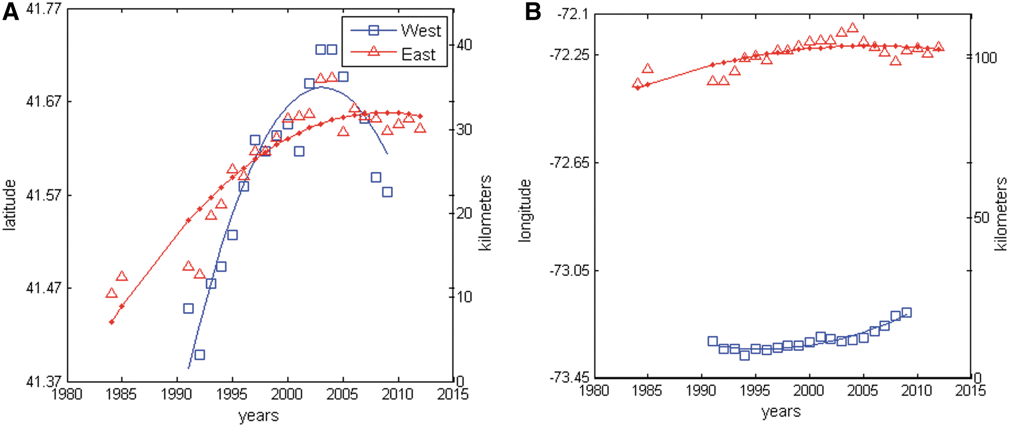
Despite two separate introductions, the yearly fluctuations in number of Lyme disease cases are similar in both parts of the state (Fig. 1). Yearly Lyme disease cases generally increased until 2002, at which point they began to decline. However, in 2004 cases started to increase again in both areas until 2009. The fluctuating number of yearly cases did not change the rate of spread as measured by the shifts in yearly weighted geographic means of Lyme disease incidence (Fig. 2B). After establishment, increased Lyme disease incidence at the spreading edge of the epidemic pulled both geographic means northward, although the majority of cases remained in the south where the higher population density resides (Fig. 3A). With few cases in central Connecticut there was little east or west spread in the yearly geographic means (Fig. 3B).

In the eastern Connecticut region, as the epidemic progressed, the yearly shift in geographic mean (rate of epidemic expansion) decreased each year until 2007, at which point the epidemic had encompassed the entire eastern portion of the state and reached equilibrium. The equilibrium correlates to a transition from spread of Lyme disease epidemic to stable endemic transmission and correlates to a reduction in human cases compared to the epidemic phase. The rate of geographic expansion fits a second order polynomial with latitude=−0.0004t ²+0.0189t+41.4147, R ²=0.8414 and longitude=−0.0003t ²+0.0151t −72.3871 (t=1, 2, 8,…., 29), R ²=0.5998 (Fig. 3A, B).

Similarly, in western Connecticut, the parabolic shape of the yearly geographic means indicates that the epidemic quickly spread northward after establishment in the south (Fig. 3A). However, the steep curve indicates a more rapid spread than in the east, and cases had spread throughout western Connecticut by 2003. After the epidemic spread to all of western Connecticut, the total number of yearly cases declined, the geographic mean shifted back to the south, and the case distribution was no longer significantly spatially correlated. Therefore, the equilibrium shifted back toward the center of the western region as the epidemic transitioned to endemic transmission. The rate of geographic expansion fits second order polynomials with latitude=−0.0021t ²+0.0539t+41.3316, R ²=0.8510 and longitude=0.0007t ² − 0.0077t − 73.3209 (t=1,2,3,…19), R ²=0.8998 (Fig. 3A, B).

Discussion

This analysis of Lyme disease case data in Connecticut revealed strong spatial structuring of two disease clusters, indicating two spatially and temporally independent foci of origin and a recent shift from rapid epidemic Lyme disease spread throughout the state to lower and more stable endemic transmission. Lyme disease has spread uncontrolled throughout the state, and understanding the spatial and temporal spread may aid in predicting current and future risks to guide interventions and mitigation strategies.

In 1977, Lyme disease was first identified in Lyme, Connecticut (Steere et al. 1978) and firmly established before the 1984 survey determined significant spatial clustering around East Haddam. In contrast, the western Connecticut cluster did not become spatially autocorrelated until 1991, and the cluster centered in Newtown. The original sources of I. scapularis for both Connecticut epidemic clusters are likely white-tailed deer introduced from a refuge on Long Island after their extermination from the mainland during the 19^th century (Halls 1984). Prior to 1984, I. scapularis was abundant only in the region of Lyme, Connecticut (Wallis et al. 1978, Petersen et al. 1989), and these likely arrived from deer swimming in the Long Island Sound (Halls 1984). In contrast, the western Connecticut epidemic likely originated during the 1980s from the expanding Lyme disease epidemic in Westchester County, New York, which is immediately adjacent to Newtown, Connecticut (Williams et al. 1986, White et al. 1991). Furthermore, white-tailed deer examined in western Connecticut for the presence of I. scapularis or antibodies to B. burgdorferi yielded negative results prior to 1988 (Anderson and Magnarelli 1980, White et al. 1991).

Two separate introductions of Lyme disease explain the case distribution and rapid spread throughout the state better than a single introduction in the eastern half of the state because the Connecticut River running north to south through central Connecticut separates the eastern and western clusters. Peterson et al. (1989) hypothesized the river stopped the spread of deer and the disease east and west. Furthermore, this physical barrier was previously shown to impede the easterly spread of diseases such as raccoon rabies to townships lying west of the river (Lucey et al. 2002, Smith et al. 2002, 2005). For Lyme disease to appear in an area, three elements are necessary: Lyme disease bacteria (Borrelia), ticks that transmit the disease (I. scapularis), and mammalian hosts for the pathogen and ticks (such as mice and deer) (Turney et al. 2014). The river may impede the spread of mice and small mammals, which are alternative hosts.

The yearly case distributions also indicate a northward expansion during the epidemic phase, which is characterized by high incidence and geographic expansion. The large population in southeastern Connecticut obscured the expansion of the disease north in previous studies because the majority of cases remain in the more populated areas. However, by using the weighted geographic mean analysis with incidence data, various population sizes of each town are accounted. The end of the epidemic phase is characterized by a decreasing rate of spread indicated by the movement of the weighted geographic mean and a reversion of the geographic mean toward the middle of the state. During the endemic phase, the number of Lyme disease cases is more proportional to the population. Therefore, more cases are reported in the more heavily populated southern areas of the state. In western Connecticut where the epidemic was more recent, the geographic rate of expansion was greater as indicated by the steeper slope. In contrast, in eastern Connecticut, the epidemic was slower and more stable due to establishment of Lyme disease from an earlier introduction in Connecticut. The epidemic to endemic transition was observed in both the eastern and western epidemics.

All surveillance activity is subject to human variation and reporting bias, as well as other factors such as changing case definitions and fluctuations in reporting of a novel condition or during an epidemic, rather than after the transition to endemic disease transmission. Throughout this study, the data were gathered using passive surveillance, active surveillance, enhanced laboratory, and mandatory laboratory surveillance by the Connecticut Department of Public Health. The reporting requirements and methods greatly influenced the number of cases reported each year (Connecticut Health Department 2005). However, the geographic distribution of the cases and the trend in weighted geographic means remained consistent in both eastern and western Connecticut during the epidemics and transitions to endemic transmission. Therefore, spatial analysis of epidemiological data for vector-borne zoonosis, such as Lyme disease, provides valuable insights into underlying processes of disease spread such as disease vector distributions and normalized incidence of epidemic versus endemic transmission. Last, spatial and temporal risk analysis based on epidemic expansion rates can help predict current and future risk. In at risk areas, prompt recognition and treatment of the disease and prevention measures, such as personal protection, habitat manipulation, and vector control can be implemented to reduce the hazard.

Conclusions

Historical case records were used to identify two geographically and temporally distinct introductions of Lyme disease into Connecticut. The two introductions have high statistical clustering and a uniform direction and rate of spread until equilibriums were established in both eastern and western Connecticut. This study confirms the importance of the Connecitcut River dividing the state and the introductions from Long Island. Furthermore, the results demonstrate Lyme disease spread rapidly throughout the state during an epidemic phase of high incidence and then transitioned to an endemic phase in recent years, which is characterized by a lower incidence.

Footnotes

Acknowledgments

Funding and support had no influence on the findings or the investigators. This research was funded by US Department of Agriculture (USDA), the Agricultural Research Service with Specific Cooperative Agreement 58-5430-1-0356. The funding agency had no input in study design and conduct of the study; collection, management, analysis, and interpretation of the data; preparation, review, or approval of the manuscript; or decision to submit the manuscript for publication. The Lyme disease case data are publically available either in the publication of (Petersen et al. ) or on the Connecticut Department of Public Health (CDPH) website. As such, Lee W. Cohnstaedt, PhD, at the USDA Agricultural Research Service had full access to all the data in the study and takes responsibility for the integrity of the data and the accuracy of the data analysis. The data were analyzed by Ling Xue and Caterina Scoligo, PhD, at Kansas State University and Lee W. Cohnstaedt. The manuscript was written and reviewed by Ling Xue, Caterina Scoligo, David S. McVey, PhD, Rebecca Boone, and Lee W. Cohnstaedt.

Author Disclosure Statement

No competing financial interests exist.

References

Anderson

, Magnarelli

. Vertebrate host relationships and distribution of ixodid ticks (Acari: Ixodidae) in Connecticut, USA. J Med Entomol, 1980; 17:314–323.

Boots

, Tiefelasdorf

. Global and local spatial correlation in bounded regular tessellations. J Geograph Syst, 2000; 2:319–348.

Centers for Disease Control and Prevention (CDC). Case definitions for infectious conditions under public health surveillance. MMWR Morb Mortal Wkly Rep, 1997; 46:20–21.

Childs

, Krebs

, Real

, Gordon

. Animal-based national surveillance for zoonotic disease: Quality, limitations, and implications of a model system for monitoring rabies. Prev Vet Med, 2007; 78:246–261.

Connecticut Health Department. Lyme Disease—Connecticut. Connecticut Epidemiologist, 2005; 26:13–14.

Eisen

, Piesman

, Zielinski-Gutierrez

, Eisen

. What do we need to know about disease ecology to prevent Lyme disease in the northeastern United States?. J Med Entomol, 2012; 49:11–22.

Ertel

, Gacek

, Nelson

, Cartter

. Lyme disease—Connecticut. Connecticut Epidemiologist, 2007; 28:5–8.

Ertel

, Nelson

, Cartter

. Effect of surveillance method on reported characteristics of Lyme disease, Connecticut, 1996–2007. Emerg Infect Dis, 2012; 18:242–247.

Falco

, McKenna

, Daniels

, Nadelman

, et al. Temporal relation between Ixodes scapularis abundance and risk for Lyme disease associated with erythema migrans. Am J Epidemiol, 1999; 149:771–776.

10.

Glavanakov

, White

, Caraco

, Lapenis

, et al. Lyme disease in New York State: Spatial pattern at a regional scale. Am J Trop Med Hyg, 2001; 65:538–545.

11.

Halls

. White-Tailed Deer: Ecology and Management. Harrisburg, PA: Stackpole Books, 1984.

12.

Kitron

, Kazmierczak

. Spatial analysis of the distribution of Lyme disease in Wisconsin. Am J Epidemiol, 1997; 145:558–566.

13.

Lastavica

, Wilson

, Berardi

, Spielman

, et al. Rapid emergence of a focal epidemic of Lyme disease in coastal Massachusetts. N Engl J Med, 1989; 320:133–137.

14.

Lucey

, Russell

, Smith

, Wilson

, et al. Spatiotemporal analysis of epizootic raccoon rabies propagation in Connecticut, 1991–1995. Vector Borne Zoonotic Dis, 2002; 2:77–86.

15.

Petersen

, Sweeney

, Checko

, Magnarelli

, et al. Epidemiological and clinical features of 1,149 persons with Lyme disease identified by laboratory-based surveillance in Connecticut. Yale J Biol Med, 1989; 62:253–262.

16.

Smith

, Lucey

, Waller

, Childs

, et al. Predicting the spatial dynamics of rabies epidemics on heterogeneous landscapes. Proc Natl Acad Sci USA, 2002; 99:3668–3672.

17.

Smith

, Waller

, Russell

, Childs

, et al. Assessing the role of long-distance translocation and spatial heterogeneity in the raccoon rabies epidemic in Connecticut. Prev Vet Med, 2005; 71:225–240.

18.

Stafford

, Cartter

, Magnarelli

, Ertel

, et al. Temporal correlations between tick abundance and prevalence of ticks infected with Borrelia burgdorferi and increasing incidence of Lyme disease. J Clin Microbiol, 1998; 36:1240–1244.

19.

Steere

. Diagnosis and treatment of Lyme arthritis. Med Clin North Am, 1997; 81:179–194.

20.

Steere

, Malawista

, Snydman

, Shope

, et al. Lyme Arthritis: An epidemic of oligoarticular arthritis in children and adults in three Connecticut communities. Arthritis Rheum, 1977; 20:7–17.

21.

Steere

, Broderick

, Malawista

. Erythema chronicum migrans and Lyme arthritis: Epidemiologic evidence for a tick vector. Am J Epidemiol, 1978; 108:312–321.

22.

Steere

, Gibofsky

, Patarroyo

, Winchester

, et al. Chronic Lyme arthritis. Clinical and immunogenetic differentiation from rheumatoid arthritis. Ann Intern Med, 1979; 90:896–901.

23.

Turney

, Gonzalez

, Millien

. The negative relationship between mammal host diversity and Lyme disease incidence strengthens through time. 2014; 95:3244–3250.

24.

Wallis

, Brown

, Kloter

, Main

Jr . Erythema chronicum migrans and Lyme arthritis: Field study of ticks. Am J Epidemiol, 1978; 108:322–327.

25.

White

, Chang

, Benach

, Bosler

, et al. The geographic spread and temporal increase of the Lyme disease epidemic. JAMA, 1991; 266:1230–1236.

26.

Williams

, Curran

, Lee

, Sousa

. Lyme disease: Epidemiologic characteristics of an outbreak in Westchester County, NY. Am J Public Health, 1986; 76:62–65.