Measurement of Striatal and Extrastriatal Dopamine D 1 Receptor Binding Potential With [ 11 C]NNC 112 in Humans: Validation and Reproducibility

Human subjects

We report here the results of six consecutive weekly experiments. Six healthy volunteers participated in this study (age 33 ± 9 years, range 23 to 45 years; these and subsequent values given as means ± SD; five men and one woman). All subjects were scanned twice on the same day to evaluate the reproducibility of the outcome measures. The study was approved by the Columbia Presbyterian Medical Center Institutional Review Board, and subjects provided written informed consent after receiving an explanation of the study. The absence of pregnancy and medical, neurological, and psychiatric history (including alcohol and drug abuse) was assessed by history, review of systems, physical examination, routine blood tests including pregnancy test, urine toxicology, and electrocardiography.

Radiochemistry

[¹¹C]NNC 112 was prepared by N-methylation of the precursor using [¹¹C]methyltriflate as previously described (Halldin et al., 1998). Specific radioactivity at the time of injection was 1,255 ± 355 Ci/mmol (n = 12, range from 883 to 2,195 Ci/mmol). Injected dose was 15.0 ± 2.3 mCi (n = 12, range from 11.8 to 18.2 mCi).

Positron emission tomography protocol

Subject preparation included placement of arterial and venous catheters, fiducial markers, and polyurethane head immobilizer. An arterial catheter was inserted in the radial artery after completion of the Allen test and infiltration of the skin with 1% lidocaine. A venous catheter was inserted in a forearm vein on the opposite side. Four fiducial markers filled with ¹¹C (∼3 μCi/marker at the time of injection) were glued on the subject's head. Head movement minimization was achieved with a polyurethane head immobilizer system (Soule Medical, FL, U.S.A.) molded around the head of the subject. This system provides better restraint than a thermoplastic mask (unpublished data). The PET imaging was performed with the ECAT EXACT 47 (Siemens/CTI, Knoxville, TN, U.S.A.; 47 slices covering an axial field of view of 16.2 cm, axial sampling of 3.375 mm, three-dimensional mode in-plane and axial resolution of 6.0 and 4.6 mm full width at half-maximum at the center of the field of view, respectively) (Wienhard et al., 1992). A 10-minute transmission scan was obtained before radiotracer injection. [¹¹C]NNC 112 was injected intravenously over 45 seconds. Emission data were collected in the three-dimensional mode for 120 minutes as 21 successive frames of increasing duration (3 × 20 s, 3 × 1 min, 3 × 2 min, 2 × 5 min, 10 × 10 min). Images were reconstructed to a 128 × 128 matrix (pixel size of 2.5 × 2.5 mm²). Reconstruction was performed with attenuation correction using the transmission data and a Sheppe 0.5 filter (cutoff 0.5 cycle/projection rays). Subjects were allowed to rest outside of the camera for 15 to 30 minutes between the two injections.

Input function measurement

After radiotracer injection, arterial samples were collected every 5 seconds with an automated sampling system for the first 2 minutes (Graham and Lewellen, 1993) and manually thereafter at longer intervals. A total of 31 samples were obtained per experiment. After centrifugation (10 minutes at 1,800 g), plasma was collected in 200-μL aliquots and counted in a gamma counter (Wallac 1480 Wizard 3M Automatic Gamma Counter). Gamma counter efficiency was calibrated at regular intervals with the PET camera using an ¹⁸F solution. In addition, a long-lived source (²²Na) was counted with each set of samples to control for between-run variance in counting efficiency.

Six selected samples (collected at 2, 8, 16, 30, 50, and 70 minutes) were further processed by protein precipitation using acetonitrile followed by high-pressure liquid chromatography to measure the fraction of plasma activity representing unmetabolized parent compound. Plasma samples (0.5 mL) were added to 0.7 mL of acetonitrile in a centrifuge tube. After mixing, the samples were centrifuged at 14,000 rpm for 3.5 minutes. The acetonitrile solution was separated and analyzed by high-pressure liquid chromatography. The system consisted of a Waters 510 isocratic pump, a Rheodyne injector with a 2-mL loop, a Phenomenex C18 ODS column (10-μm particle size, 250 × 4.6 mm, stainless steel), and a gamma detection system (Bioscan Flow Count unit). The column was eluted with a solvent mixture of acetonitrile/0.1 mol/L aqueous ammonium formate (30:70) at a flow rate of 2.5 mL/min. Five fractions collected over 12 minutes were counted. A standard [¹¹C]NNC 112 solution was processed with each experiment. Parent eluted with fractions 3 and 4. For each sample, the fraction parent was estimated by the ratio of decay-corrected activity in collections 3 and 4 to that in the total collection.

A biexponential function was fitted to the six measured fractions parent and used to interpolate values between and after the measurements. The smallest exponential of the fraction parent curve, λ_par, was constrained to the difference between λ_cer, the terminal rate of washout of cerebellar activity, and λ_tot, the smallest elimination rate constant of the total plasma (Abi-Dargham et al., 1999). The input function was calculated by the product of total counts and interpolated fraction parent at each time. The measured input function values [C_a(t); μCi/mL) were fitted to a sum of three exponentials, and the fitted values were used as input to the kinetic and graphical analyses. The clearance of the parent compound (C_L; L/h) was calculated as the ratio of the injected dose to the area under the curve of the input function (Abi-Dargham et al., 1994).

For the determination of the plasma free fraction (f₁), triplicate 200-μL aliquots of plasma collected before injection were mixed with radiotracer, pipetted into ultrafiltration units (Centrifree, Amicon, Danvers, MA, U.S.A.), and centrifuged at room temperature (20 minutes at 4,000 rpm). At the end of centrifugation, plasma and ultrafiltrate activities were counted, and f₁ was calculated as the ratio of ultrafiltrate to total activity concentrations (Gandelman et al., 1994). Triplicate aliquots of saline solution mixed with radiotracer were also processed to determine the filter retention of free [¹¹C]NNC 112.

Magnetic resonance imaging acquisition and segmentation procedures

Magnetic resonance imaging (MRI) was performed on a GE 1.5 T Signa Advantage system (Milwaukee, WI, U.S.A.). After a sagittal scout (localizer) image performed to identify the anterior-posterior commissural (AC-PC) plane (1 minute), a transaxial T1-weighted sequence with 1.5-mm slice thickness was acquired in a coronal plane orthogonal to the AC-PC plane over the whole brain with the following parameters: three-dimensional SPGR (spoiled gradient-recalled acquisition in the steady state); repetition time 34 milliseconds; echo time 5 milliseconds; flip angle 45°; slice thickness 1.5 mm and zero gap; 124 slices; field of view 22 × 16 cm; 256 × 192 matrix, reformatted to 256 × 256, yielding a voxel size of 1.5 × 0.9 × 0.9 mm; and time of acquisition 11 minutes.

The MRI segmentation was performed within MEDx (Sensor Systems, Sterling, VA, U.S.A.), with original subroutines implemented in MATLAB (Math Works, Natick, MA, U.S.A.). Steps for MRI segmentation included correction for field inhomogeneities, fitting of the voxel distribution to a combination of three Gaussians functions, voxel classification, and postfiltering. To correct for field inhomogeneity, histograms of one anterior coronal slice and one posterior coronal slice were computed, as described below. g _x was defined as the difference in peak locations divided by the distance between slices. In a similar manner, g _y was defined from two sagittal slices, and g _z was defined from two transaxial slices. Next, an image G was constructed of the same dimensions as the MR image, with G being an affine function with gradient (g _x , g _y , g _z ). Gradient-corrected MRI of the image I was given by I/G. The principal advantage of this approach is that if there is no gradient inhomogeneity, the gradient correction causes no loss of resolution. Gradient-corrected images were then imported into MATLAB. Voxel intensity distribution was fit to a linear combination of three Gaussian functions:

N ( x ) = ∑ k = 1 3 α k 1 ( 2 π σ k ) 1 / 2 exp [ − 1 2 ( x − μ k σ k ) 2 ]

(1)

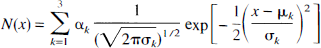
where α _k , μ _k , and σ _k are the weight, mean, and SD of the Gaussian function for compartment k. The values of these parameters were estimated using maximum likelihood (Fig. 1), and the threshold values were used in the MEDx system to perform the segmentation of the MRI into gray matter (GM), white matter (WM), and cerebrospinal fluid (CSF) compartments. These thresholds were applied to create GM, WM, and CSF masks. The masks were finally smoothed and thresholded to remove isolated voxels.

OPEN IN VIEWER

FIG. 1.

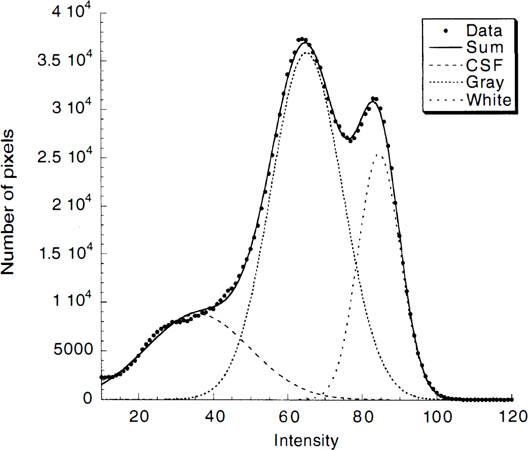
Distribution of voxel intensity from a T1-weighted SPGR (spoiled gradient-recalled acquisition in the steady state) magnetic resonance imaging file and fitted sum of three Gaussians estimating voxel intensity of cerebrospinal fluid and gray and white matter. The solid line represents the sum of the fitted Gaussians. The intersection between the Gaussians was used as threshold for pixel classification.

Image analysis

Image analysis was performed with MEDx according to the following steps: frame realignment, PET-MRI registration, and time-activity curve measurement.

1. Frame realignment. To correct for head movement during the acquisition, all frames were coregistered to the first frame of the study, using a least-squares algorithm for within-modality coregistration (automated image registration) (Woods et al., 1992). Images were thresholded to the level of the ¹¹C fiducial markers, and only the signals from the markers were used for automated image frame-to-frame registration. The x, y, and z coordinates of the pixel with highest intensity of each fiducial marker were used to monitor the quality of between-frame coregistration.

2. PET-MRI registration. After frame-to-frame registration, the 21 frames were summed, and the summed PET image was coregistered and resampled to the MR image, using automated image registration (Woods et al., 1992). The summed PET image was used for the coregistration because it contains counts from the initial flow-dependent activity distributions that enhance detection of boundaries of regions with low receptor density, such as the cerebellum. The parameters of the spatial transformation matrix of the summed PET data set were then applied to each individual frame. Thus, each PET frame was resampled in the coronal plane to a voxel volume of 1.5 × 0.9 × 0.9 mm³.

3. Region-of-interest (ROI) tracing and activity sampling. The ROI boundaries were drawn on the MR image according to criteria based on brain atlases (Talairach and Tournoux, 1988; Duvernoy, 1991) and on published reports (Pani et al., 1990; Kates et al., 1997; Killiany et al., 1997). Neocortical regions included dorsolateral prefrontal cortex (DLPFC), medial prefrontal cortex, orbitofrontal cortex (OFC), anterior cingulate cortex, parietal cortex, temporal cortex, and occipital cortex. Subcortical regions included caudate, putamen, thalamus, amygdala, hippocampus, and cerebellum. Two methods were used for final ROI definition. A segmentation-based method was used for neocortical regions, and a direct identification method was used for subcortical regions. For neocortical regions, “large” regions were first drawn to delineate the boundaries of the ROIs. Within these regions, only the voxels classified as GM were used to measure activity distribution. This process is illustrated in Fig. 2 for DLPFC and OFC. Because of the mixture of GM and WM in central gray structures (especially thalamus), the segmentation-based approach was not used to define subcortical ROIs, and the boundaries of these regions were identified by anatomical criteria.

OPEN IN VIEWER

FIG. 2.

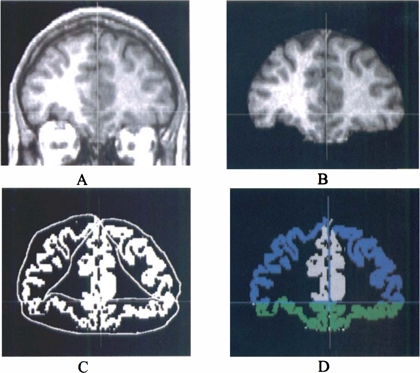
The process of region-of-interest (ROI) definition for dorsolateral prefrontal cortex (DLPFC) and orbitofrontal cortex (OFC) in one coronal plane. (A) Original magnetic resonance (MR) image [coronal plane, perpendicular to anterior-posterior commissural (AC-PC) plane, 5 mm anterior to the anterior part of the genu of corpus callosum]. The vertical line is the midsagittal section, and the horizontal line is the AC-PC plane. (B) MR image after removal of extracerebral tissue. (C) Same image as B after segmentation, with only gray matter (GM) represented. Lines represent boundaries of ROIs. Two ROIs are defined on each side: Above the AC-PC plane and excluding the medial gray is the DLPFC. Below the AC-PC plane is the OFC. (D) GM voxels are assigned to ROIs if included within ROI boundaries: blue, DLPFC; green, OFC.

Quantitative analysis

Derivation of [¹¹C]NNC 112 regional distribution volumes was performed using kinetic and graphical analyses. A three-compartment model (i.e., two-tissue compartment model) provided the general framework for each method. The model included the arterial plasma compartment (C_a), the intracerebral free and nonspecifically bound compartment (nondisplaceable compartment; C₂), and the specifically bound compartment (C₃). The equilibrium distribution volume of a compartment i (V _i ; mL/g) was defined as the ratio of the tracer concentration in this compartment to the free plasma concentration at equilibrium:

V i = C i f 1 C a

(2)

V₂ and V₃ were defined as the distribution volumes of the second (nondisplaceable) and third (specific) compartments, respectively. V₃ is equal to BP (g/mL), which is the ratio of the receptor density (B_max; nmol/L/g of tissue) and affinity (K_D; nmol/L/mL of brain water) (Mintun et al. 1984; Laruelle et al. 1994d). V_T was defined as the total regional equilibrium distribution volume, equal to the sum of V₂ and V₃. Both kinetic and graphical analyses shared two assumptions: given the negligible concentration of D₁ receptors in the cerebellum (Hall et al., 1994), cerebellar V_T was assumed to represent only free and nonspecific binding and to provide a reasonable estimate of V₂ in the ROIs; the contribution of plasma total activity to the regional activity was calculated assuming a 5% blood volume in the ROIs (Mintun et al., 1984).

Kinetic analysis

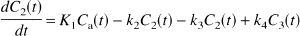
Kinetic analysis was performed according to the differential equations:

d C 2 ( t ) d t = K 1 C a ( t ) − k 2 C 2 ( t ) − k 3 C 2 ( t ) + k 4 C 3 ( t )

(3)

d C 3 ( t ) d t = k 3 C 2 ( t ) − k 4 C D 3 ( t )

(4)

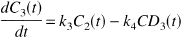
with the kinetic parameters defined as

K 1 = F E = F ( 1 − e − P S / F ) ( mL g − 1 min − 1 )

(5)

k 2 = K 1 V 2 f 1 ( min − 1 )

(6)

k 2 = k on B max ′ V 2 ( min − 1 )

(7)

k 4 = k off ( min − 1 )

(8)

where F (mL g⁻¹ min⁻¹) is the regional blood flow, E (unitless) the unidirectional extraction fraction, PS (mL g⁻¹ min⁻¹) the permeability-surface area product of the tracer, k_on [(nmol/L)⁻¹ min⁻¹] the bimolecular ligand-receptor association rate constant, B_max′ (nmol/L) the concentration of receptors available for binding (equal to B_max as experiments were performed at tracer dose), and k_off (min⁻¹) the receptor dissociation rate constant. Kinetic parameters were derived by nonlinear regression using a Levenberg-Marquart least-squares minimization procedure (Levenberg, 1944) implemented in MATLAB, as previously described (Laruelle et al., 1994c). In the absence of precise knowledge of the variance associated with the measurement of each frame, uniform weighting was used in the regression (Carson, 1986; Burger and Buck, 1997). Goodness of fit of models with different levels of complexity was compared using the Akaike information criterion (Akaike, 1974) and the F test (Landlaw and DiStefano, 1984; Carson, 1986).

In the ROIs, volumes of distribution were then calculated according to

V 2 = K 1 k 2 f 1

(9)

and

V 3 = K 1 k 3 k 2 k 4 f 1 = BP

(10)

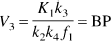
Substituting in Eq. 10 the terms K₁/k₂f₁, k₃, and k₄ with Eqs. 5, 6, and 7, respectively, and recalling that K_D = k_off/k_on establish the equivalence between V₃ and BP (Laruelle et al., 1994a).

The BP, as defined above, is the only expression of BP that is dependent on receptor parameters (i.e., K_D and B_max) and can be compared with in vitro values (see derivations in Laruelle et al., 1994a). Another outcome measure of interest is the specific-to-nonspecific equilibrium partition coefficient, termed k₃/k₄ or V₃″ (Laruelle et al., 1994d):

k 3 k 4 = BP V 2

(11)

k₃/k₄ is often used as the outcome measure in the PET literature and is referred to as the BP (Gjedde and Wong, 1990; Logan et al., 1990). In fact, this ratio does not correspond to BP (=B_max/K_D) as classically defined by Mintun et al. (1984) but to the ratio of BP to V₂, as shown by dividing Eq. 10 by Eq. 9 (Eq. 11). To avoid confusion, we use BP to designate the “true” BP, as defined in Eq. 10, and k₃/k₄ to designate the “practical” BP, as defined in Eq. 11.

The ratio of total to nonspecific distribution volume is termed the DVR:

DVR = V T V 2 = k 3 k 4 + 1

(12)

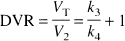
DVR is reported to facilitate comparison with results of studies reporting reproducibility of [¹¹C]raclopride DVR (Volkow et al., 1993), [¹⁸F]altanserin DVR (Smith et al., 1998), and [¹¹C]SCH 23390 DVR (Chan et al., 1998).

Results from kinetic analysis were evaluated with four criteria: identifiability, validity, stability, and reliability.

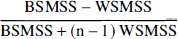
Identifiability. The term “identifiability” refers to the error in the parameter estimation due to the inherent uncertainty of this estimation. The identifiability was assessed by the standard error of the parameter at convergence. The standard error of the parameters was given by the diagonal of the covariance matrix (Carson, 1986) and expressed as percentage of the parameters (coefficient of variation; %CV). This standard error should not be confused with the variance of the parameter in the investigated population (between-subject SD or %CV) or with the lack of reproducibility (within-subject SD or %CV). It should also be noted that uniform weighting of the least-squares estimation might be associated with an overestimation of the standard error of the parameters if the measurement variances range over orders of magnitude (Carson, 1986).

Reliability. The test/retest variability was calculated as the absolute value of the difference between test and retest values, expressed as percentage of the mean value of both measurements. To evaluate the within-subject variability relative to the between-subject variability, both within-subject SD and between-subject SD were calculated and expressed as percentage of mean value (within-subject %CV and between-subject %CV). The reliability of the measurements was assessed by the intraclass correlation coefficient (ICC) calculated as follows (Kirk, 1982):

BSMSS − WSMSS BSMSS + ( n − 1 ) WSMSS

(13)

where BSMSS is the mean sum of squares between subjects, WSMSS is the mean sum of squares within subjects, and n is the number of repeated observations (n = 2 in this study). This coefficient estimates the reliability of the measurement and assumes values from −1 (no reliability; i.e., BSMSS = 0) to 1 (maximum reliability, achieved in case of identity between test and retest; i.e., WSMSS = 0).

Graphical analysis

Regional time-activity curves were graphically analyzed according to the equation

∫ 0 t C ROI ( t ) d t C ROI ( t ) = a ∫ 0 t f 1 C a ( t ) d t C ROI ( t ) + b

(14)

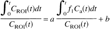
where the values of the slope a and the intercept b were obtained by linear regression (Logan et al., 1990). This method allows the determination of regional V_T of reversible ligands as the slope of the regression line without assuming a particular compartmental configuration. Assuming, as in the kinetic analysis, the equivalence between the cerebellum distribution volume (V_{T cer}) and the nondisplaceable distribution volume in the ROI, outcome measures were calculated as

BP = V T ROI − V T cer

(15)

DVR = V T ROI V T cer

(16)

and

k 3 k 4 = DVR − 1

(17)

Reliability of the graphical analysis was evaluated as described for the kinetic analysis.

Noise analysis

Simulations were performed to evaluate the sensitivity of the kinetic and graphical analysis to experimental noise. This analysis was carried out for the cerebellum and one ROI (caudate). First, noise-free data [T(t)] were created, using a standard input function and a standard impulse response function. Data were simulated for 120 minutes, with values calculated every minute (n = 120). Second, various levels of random noise were introduced into the data. Due to the rapid decay of ¹¹C, the noise increased over the course of an experiment, and the simulated noise was designed to reflect this effect. For noise level {α _j }, a normal random noise vector with mean 1 and SD at time t equal to α _j [exp(τt)/SD of exp(τt)] was generated, where τ was the exponent associated with ¹¹C half-life [20 minutes, τ = 0.034 = ln (2)/20]. The “true” datum T(t) was multiplied at each point by the noise vector, resulting in a “measured” data set M(t) with mean = T(t) and SDj(t) = T(t)α _j [exp(0.034t)/SD of exp(τt)]. At each noise level α _j , this operation was repeated 500 times. Each data set was analyzed with kinetic or graphical analysis. The average V_T derived from these noisy data sets was compared with the true value to estimate the bias introduced by the noise in the derivation of V_T, whereas the SD provided a measure of the noise-related error in V_T.

Statistical analysis

For each outcome measure and each subject (n = 6), the average of test and retest values was calculated, and results are given as means ± SD of these six average measurements. Thus, unless otherwise specified, SD refers to between-subject SD, that is, to the estimated variability in the investigated population (each subject counts only once, n = 6). When the SD refers to variability between the experiments rather than between subjects (such as for the injected dose), the SD is followed by n = 12. Statistical analysis was performed with repeated-measures analysis of variance. Relationships between continuous variables were analyzed with the Pearson product-moment correlation coefficient. A two-tailed probability value of 0.05 was selected as the significance level.

Plasma analysis

[¹¹C]NNC 112 underwent rapid metabolism measured in human plasma (Fig. 3). At 30 minutes, only 18 ± 6% (n = 12) of the total activity corresponded to the parent compound. The six measures (2, 8, 16, 30, 50, and 70 minutes) of fraction parent were fit to a sum of two exponentials. In all cases, the unconstrained fit of the fraction parent curve yielded a value of 0 for the smallest exponent (λ_par). This solution was consistent with the low rate of metabolism after 30 minutes and the absence of data after 70 minutes. However, this solution was not consistent with the observation of a faster washout rate in the cerebellum compared with the total plasma activity after 30 minutes. This problem was addressed by constraining λ_par to the difference between λ_cer, the terminal rate of washout of cerebellar activity, and λ_tot, the smallest elimination rate constant of the total plasma. For each experiment, the terminal cerebellar washout rates were calculated by fitting the cerebellum data from 30 to 120 minutes to a one-exponential function (λ_cer = −0.00764 ± 0.00287 min⁻¹, n = 12). Similarly, the smallest exponential of the total plasma activity was derived by fitting the total plasma activity from 30 to 120 minutes to one exponential (λ_tot = −0.00322 ± 0.00083 min⁻¹, n = 12). The smallest exponential of the fraction parent curve was constrained to the difference between the two functions λ_cer and λ_tot (−0.00450 ± 0.00296 min⁻¹, n = 12), and this fit was used to correct total activity by the fraction parent.

OPEN IN VIEWER

FIG. 3.

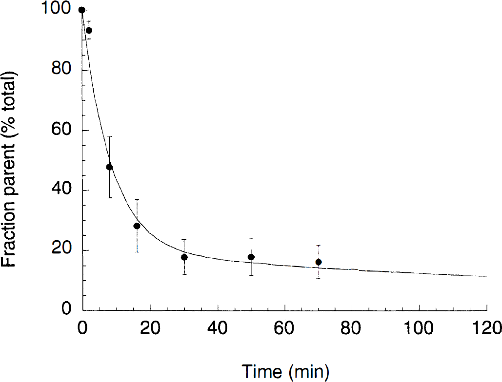
Fraction of plasma activity associated with parent compound (% total) following [¹¹C]NNC 112 injection in humans. Each point is the average ± SD of 12 measurements (6 subjects studied twice). The solid line represents the sum of two exponentials, with second half-life constrained to −0.00440 min⁻¹. This value corresponded to the average value of the difference between cerebellum and total plasma terminal half-lives.

The input function was fit to a sum of three exponentials (Fig. 4), and fitted values were used as input function for kinetic and graphical analysis. The average [¹¹C]NNC 112 plasma clearance was 96 ± 31 L/h. Significant between-subject differences in plasma clearance were detected (P = 0.006). Test/retest variability of the clearance measurement was 15 ± 8%, and its reliability was excellent with within-subject %CV of 10%, between-subject %CV of 32%, and ICC of 0.83.

OPEN IN VIEWER

FIG. 4.

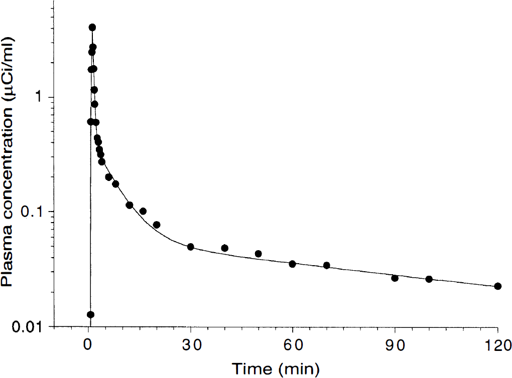
Plasma concentration of [¹¹C]NNC 112 following injection of 18 mCi in one healthy volunteer. Points represent measured values. The solid line represents the result of a three-exponential fit to the measured values. Clearance was 100 L/h.

The mean plasma f₁ fraction was 1.02 ± 0.28%. The within-subject CV of the f₁ measurement (34% CV) exceeded the between-subject CV (27%), which translated into poor reliability (ICC = −0.20). In addition, significant retention of free radiotracer on the filter was noted (the free fraction measured in saline solution was 77 ± 4%, n = 12). Because of the failure to reliably identify between-subject differences in free fraction, this correction factor was neglected, and distribution volumes were expressed relative to the total parent.

Brain uptake

Highest brain regional uptake was observed in caudate and putamen, and lowest uptake was observed in the cerebellum and thalamus (Fig. 5). In other regions (neocortex and limbic system), activity levels were intermediate between striatal and cerebellar regions. Activity peaked early in the cerebellum, neocortical, and limbic regions (<15 minutes) and later in striatum (20-40 minutes). Appreciable washout was observed in all regions, suggesting that the association and dissociation rates were fast enough to allow derivation of D₁ receptor BP within the time frame of the scan. At 60 minutes, the ROI/cerebellar activity ratios were as follows: putamen, 3.72 ± 0.58; caudate, 3.26 ± 0.58; amygdala, 1.77 ± 0.32; hippocampus, 1.48 ± 0.23; anterior cingulate, 1.78 ± 0.29; DLPFC, 1.53 ± 0.20; temporal cortex, 1.69 ± 0.33; occipital cortex, 1.30 ± 0.17; and thalamus, 1.19 ± 0.21.

OPEN IN VIEWER

FIG. 5.

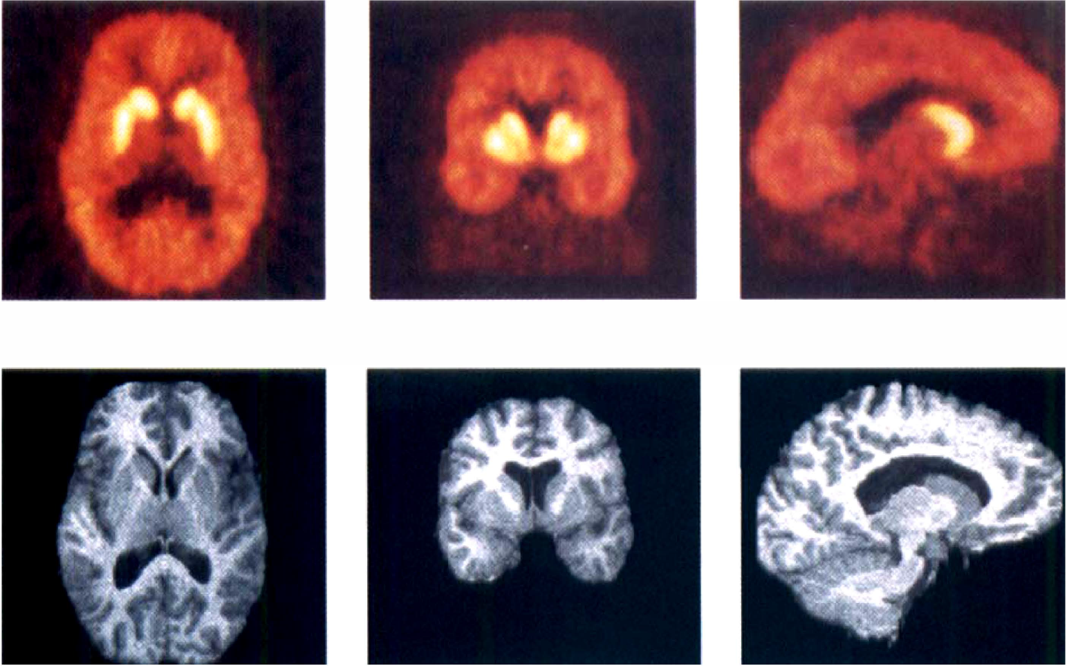
[¹¹C]NNC 112 in a human volunteer. (Top row) Positron emission tomography: Transaxial, coronal, and sagittal views of a 20-minute frame obtained 40 minutes after the injection of 16 mCi of [¹¹C]NNC 112 in a 22-year-old man. (Bottom row) Magnetic resonance imaging: SPGR (spoiled gradient-recalled acquisition in the steady state) acquisitions in the corresponding planes. Activity is concentrated in caudate, putamen, neocortex, and hippocampus. Background activity is measured in the cerebellum. Thalamic activity is very low. This distribution corresponds to the anatomical distribution of the dopamine D₁ receptors.

Kinetic analysis

Cerebellum. Cerebellar time-activity curves were fit to both a two- and a three-compartment model. In all cases, the three-compartment model provided a slightly but significantly better fit (P < 0.01; Fig. 6), with smaller values of Akaike information criterion (data not shown). Cerebellum V_T values calculated with the two- and three-compartment models were 2.54 ± 0.42 and 3.41 ± 0.58 mL g⁻¹, respectively. Thus, cerebellar V_T was 43% larger when calculated with a three-compartment model than a two-compartment model. The improved goodness of fit of the three-compartment model favored this model. However, several other factors favored the two-compartment model: (1) The identifiability of cerebellar V_T derived with a two-compartment model analysis (error of 4.13 ± 1.0%) was superior to that of the three-compartment model analysis (9.52 ± 7.13%). (2) The cerebellar V_T values derived by the Logan analysis (2.75 ± 0.48 mL g⁻¹) were closer to the two-compartment model cerebellar V_T (2.54 ± 0.42 mL g⁻¹) than the three-compartment model cerebellar V_T (3.41 ± 0.58 mL g⁻¹). (3) The stability over time of the two-compartment model was superior to that of the three-compartment model: For the two-compartment model, all values derived for periods from 60 to 120 minutes were within 10% of the reference value (= 120-minute value). In contrast, values were very unstable for the three-compartment model, with no discernible pattern over time and large standard errors (Fig. 7). (4) Derivation of cerebellar V_T by the two-compartment model was very reproducible. The test/retest variability and reliability of the two-compartment model V_T (test/retest variability = 6 ± 6%, between-subject %CV = 17%, within-subject %CV = 3%, ICC = 0.92) were much better than for the three-compartment model V_T (test/retest variability = 21 ± 23%, between-subject %CV = 17%, within-subject %CV = 19%, ICC = −0.10). Together, these data suggest that the three-compartment model cerebellar fit was unstable and sensitive to the noise associated with cerebellar measurements at the end of the experiments. For these reasons, the two-compartment model fit was selected as the fit of choice to derive cerebellar V_T.

OPEN IN VIEWER

FIG. 6.

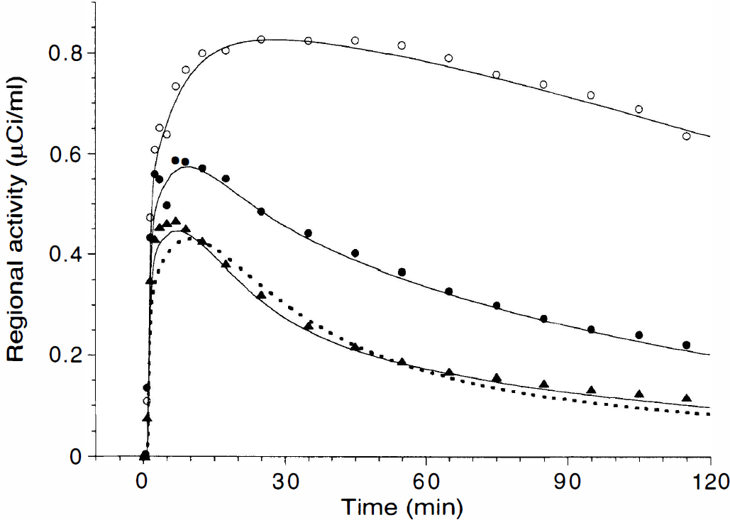
Brain time-activity curves measured in putamen (open circles), dorsolateral prefrontal cortex (filled circles), and cerebellum (triangles) after injection of 18 mCi of [¹¹C]NNC 112 (same subject as in Fig. 4). The solid line represents the results of a three-compartment model fit, and the dashed line illustrates a two-compartment model fit in the cerebellum. In the cerebellum, the three-compartment model provided a slightly but significantly better fit.

OPEN IN VIEWER

FIG. 7.

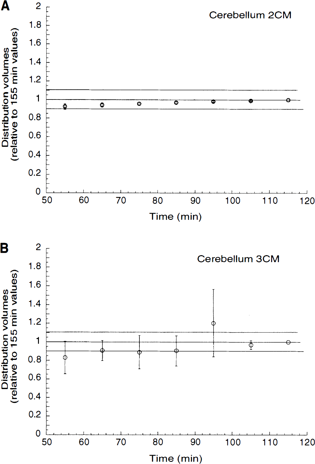
Relationship between duration of data collection and kinetic derivation of total distribution volume (V_T) in the cerebellum, according to two-compartment model (A) and three-compartment model (B).V_T values were normalized to the reference value, defined as the value measured with the whole data set (120 minutes of data collection). Each time point represents the mean ± SD of 12 determinations (6 subjects studied twice). With the two-compartment model, all values after 50 minutes were located within ± 10% of the reference values (filled columns), and the SD was very low. This result indicated that the cerebellum V_T derivation with the two-compartment model was stable and, for times of >50 minutes, practically independent of the scanning duration. In contrast, the three-compartment model presented larger deviations from the reference values, and the SD was much larger than with the two-compartment model, indicating lack of stability of the results.

Regions of interest. Data from all the other regions were fitted to a three-compartment model, with the K₁/k₂ ratio constrained to the value of the cerebellum V_T (two-compartment model). Results are presented in Table 1. The BP ranged from 8.44 ± 2.57 mL g⁻¹ (putamen) to 1.45 ± 0.41 mg g⁻¹ (thalamus). Despite these large regional differences in D₁ receptor density, the constrained model performed well in all regions.

OPEN IN VIEWER

TABLE 1.

Kinetic analysis of regional [¹¹C]NNC 112 uptake in human brain (three-compartment model constrained)

Region	K1 (mL g−1 min−1)	k2 (min−1)	k3 (min−1)	k4 (min−1)	VT (mL g−1)	BP (mL g−1)	DVR (unitless)	k3/k4 (unitless)
Caudate	0.152 ± 0.039	0.059 ± 0.008	0.132 ± 0.035	0.049 ± 0.035	10.13 ± 3.18	7.51 ± 2.98	3.89 ± 0.93	2.89 ± 0.93
Putamen	0.188 ± 0.044	0.074 ± 0.007	0.183 ± 0.083	0.057 ± 0.083	10.98 ± 2.81	8.44 ± 2.57	4.32 ± 0.80	3.32 ± 0.80
Hippocampus	0.124 ± 0.030	0.049 ± 0.007	0.015 ± 0.006	0.020 ± 0.006	4.49 ± 0.89	1.92 ± 0.77	1.77 ± 0.33	0.77 ± 0.33
Amygdala	0.112 ± 0.028	0.044 ± 0.007	0.028 ± 0.016	0.029 ± 0.016	4.90 ± 1.28	2.35 ± 1.12	1.93 ± 0.42	0.93 ± 0.42
Ant. Cingulate	0.165 ± 0.047	0.064 ± 0.011	0.037 ± 0.013	0.035 ± 0.013	5.18 ± 1.23	2.64 ± 0.98	2.04 ± 0.33	1.04 ± 0.33
DLPF Ctx	0.149 ± 0.034	0.059 ± 0.007	0.023 ± 0.007	0.030 ± 0.007	4.49 ± 1.01	1.95 ± 0.75	1.77 ± 0.27	0.77 ± 0.27
MPF Ctx	0.157 ± 0.037	0.061 ± 0.006	0.030 ± 0.007	0.033 ± 0.007	4.84 ± 1.05	2.30 ± 0.77	1.90 ± 0.26	0.90 ± 0.26
OF Ctx	0.140 ± 0.028	0.056 ± 0.010	0.028 ± 0.013	0.032 ± 0.013	4.77 ± 1.07	2.21 ± 0.97	1.89 ± 0.40	0.89 ± 0.40
Parietal Ctx	0.163 ± 0.053	0.063 ± 0.012	0.027 ± 0.010	0.032 ± 0.010	4.75 ± 1.25	2.23 ± 0.93	1.87 ± 0.31	0.87 ± 0.31
Temporal Ctx	0.139 ± 0.031	0.055 ± 0.006	0.034 ± 0.012	0.038 ± 0.012	4.86 ± 1.08	2.32 ± 0.87	1.92 ± 0.32	0.92 ± 0.32
Occipital Ctx	0.175 ± 0.044	0.069 ± 0.009	0.032 ± 0.015	0.034 ± 0.015	4.83 ± 1.09	2.29 ± 0.84	1.90 ± 0.29	0.90 ± 0.29
Thalamus	0.165 ± 0.035	0.066 ± 0.006	0.018 ± 0.005	0.032 ± 0.005	3.99 ± 0.68	1.45 ± 0.41	1.59 ± 0.16	0.59 ± 0.16
Cerebellum	0.131 ± 0.029	0.050 ± 0.008	—	—	2.54 ± 0.42	—	—	—

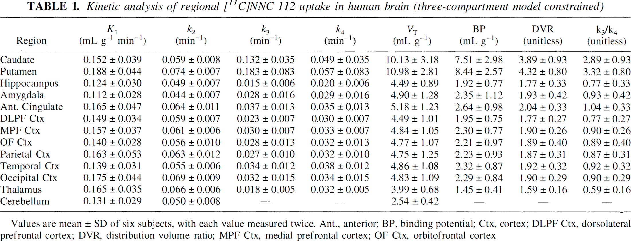
Values are mean ± SD of six subjects, with each value measured twice. Ant., anterior; BP, binding potential; Ctx, cortex; DLPF Ctx, dorsolateral prefrontal cortex; DVR, distribution volume ratio; MPF Ctx, medial prefrontal cortex; OF Ctx, orbitofrontal cortex

Identifiability. Overall, the goodness of fit was excellent, and V_T values were well identified. Regional V_T mean identifiability was 5.75 ± 6.25% (n = 144, range from 2.60 ± 0.69% in the putamen to 10.6 ± 8.43% in the hippocampus). The BP values were also well identified, with slightly more uncertainty in small-size regions (hippocampus and amygdala) or regions with lower D₁ receptor density (thalamus). The BP mean identifiability was 11.9 ± 13.0% (n = 144, range from 3.42 ± 0.98% in putamen to 24.4 ± 16.7% in thalamus). The K₁ values were very well identified in all regions (2.36 ± 0.45%, n = 144, range from 1.60 ± 0.65% in temporal cortex to 3.03 ± 1.24% in caudate). A larger but still acceptable uncertainty was associated with values of k₃ (23.4 ± 16.3%, n = 144) and k₄ (33.5 ± 27.6%, n = 144). The k₃/k₄ ratios were well identified (12.9 ± 16.1%, n = 144).

Validity. A significant relationship was observed between PET and autoradiography measures (r² = 0.97, P < 0.001) and between PET and homogenate membrane measures (r² = 0.94, P < 0.001) (Table 2).

OPEN IN VIEWER

TABLE 2.

Regional distribution of D₁ receptors in human brain: in vitro versus in vivo comparison

	In vitro
	Autoradiography*		Homogenate binding†		In vivo PET‡
Region	Specific binding fmol/mg of tissue (Mean ± SEM) n = 4	Normalized values	Bmax pmoL g−1 (Mean ± SD) n = 2–6	Normalized values	BP mL g−1 (Mean ± SD) n = 6	Normalized values
Caudate	70.7 ± 6.2	100%	11.3 ± 3.2	100%	7.5 ± 3.0	100%
Putamen	64.7 ± 8.2	92%	9.9 ± 2.1	88%	8.4 ± 2.6	112%
Hippocampus	7.8 ± 2.0	11%	1.4 ± 0.4	12%	1.9 ± 0.8	26%
Amygdala	18.4 ± 2.7	26%	2.1 ± 1.1	19%	2.4 ± 1.1	31%
Ant. Cingulate	15.5 ± 0.9	22%	1.7 ± 0.8	15%	2.6 ± 1.0	35%
DLPF Ctx	15.2 ± 0.7	21%	3.3 ± 0.8	29%	2.0 ± 0.8	26%
OF Ctx	15.9 ± 2.4	22%	—	—	2.2 ± 1.0	29%
Parietal Ctx	18.1 ± 2.1	26%	—	—	2.2 ± 0.9	30%
Temporal Ctx	—	—	2.3 ± 0.8	20%	2.3 ± 0.9	31%
Occipital Ctx	11.4 ± 2.9	16%	—	—	2.3 ± 0.8	30%
Thalamus	4.4 ± 0.6	6%	—	—	1.5 ± 0.4	19%

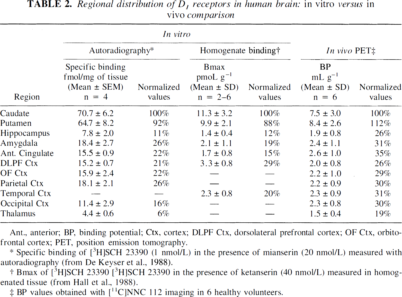
Ant., anterior; BP, binding potential; Ctx, cortex; DLPF Ctx, dorsolateral prefrontal cortex; OF Ctx, orbitofrontal cortex; PET, position emission tomography.

*

Specific binding of [³H]SCH 23390 (1 nmol/L) in the presence of mianserin (20 nmol/L) measured with autoradiography (from De Keyser et al., 1988).

†

Bmax of [³H]SCH 23390 [³H]SCH 23390 in the presence of ketanserin (40 nmol/L) measured in homogenated tissue (from Hall et al., 1988).

‡

BP values obtained with [¹¹C]NNC 112 imaging in 6 healthy volunteers.

Stability. The ROI time-activity curves were fit to shorter scanning time durations, and BP values derived from shorter scanning times were expressed relative to BP values derived with 120-minute scanning time. Average BP values were 101 ± 8% at 105 minutes (n = 120, 12 regions × 10 scans), 102 ± 8% at 95 minutes, 104 ± 8% at 85 minutes, 117 ± 42% at 75 minutes, and >120% for shorter scanning times. At 85 minutes (corresponding to a total scanning time of 90 minutes), all regions were within 10% of the reference value, with the exception of the thalamus (112 ± 30%). Figure 8 displays time-stability analyses of the caudate and the DLPFC.

OPEN IN VIEWER

FIG. 8.

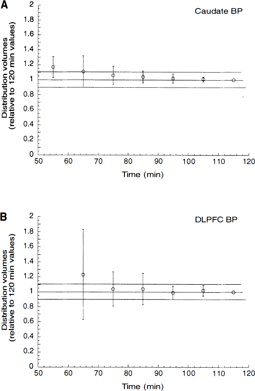
Relationship between duration of data collection and kinetic derivation of binding potential (BP) in the caudate (A) and dorsolateral prefrontal cortex (B). The BP values were normalized to the reference value, defined as the value measured with the whole data set (120 minutes of data collection). Each time point represents the mean ± SD of 12 determinations (6 subjects studied twice). For both regions, values derived after 70 minutes were within ± 10% of the reference value, and the SD became low after 90 minutes. This result suggests a good stability over time of the model after 90 minutes.

Reproducibility. The reproducibility of regional V_T and DVR are presented in Table 3. For each outcome measure, Table 3 lists the regional mean, between-subject SD (%CV), within-subject SD (%CV), test/retest variability, and ICC. For each outcome measure and each region, the between-subject SD exceeded the within-subject SD (Fig. 9). The test/retest variabilities of V_T and DVR were 8 ± 2 and 6 ± 2%, respectively. The ICC of V_T (0.91 ± 0.06) was slightly but significantly better than the ICC of DVR (0.84 ± 0.10, paired t test, P = 0.0409). The reproducibility of BP and k₃/k₄ is presented in Table 4. The test/retest variability of BP (14 ± 5%) and k₃/k₄ (13 ± 5%) was comparable and larger than for V_T (8 ± 2%) and DVR (6 ± 2%). However, for both measures, the between-subject SD exceeded the within-subject SD and the reliability was excellent (BP ICC = 0.90 ± 0.06, k₃/k₄ ICC = 0.84 ± 0.11). The reliability of BP compared with k₃/k₄ was significantly better (paired t test, P = 0.017).

OPEN IN VIEWER

TABLE 3.

Reliability of [ ¹¹ C]NNC 112 distribution volume and distribution volume ratio measurements in human brain: kinetic analysis

	Kinetic VT (mL g−1)					Kinetic DVR (unitless)
Measure parameter	Mean	BSSD (%CV)	WSSD (%CV)	VAR ± SD	ICC	Mean	BSSD (%CV)	WSSD (%CV)	VAR ± SD	ICC
Caudate	10.13	3.18 (31%)	0.41 (4%)	7% ± 02%	0.97	3.89	0.93 (24%)	0.12 (3%)	6% ± 02%	0.97
Putamen	10.98	2.81 (26%)	0.59 (5%)	10% ± 05%	0.92	4.32	0.80 (18%)	0.12 (3%)	5% ± 04%	0.96
Hippocampus	4.49	0.89 (20%)	0.32 (7%)	12% ± 12%	0.77	1.77	0.33 (19%)	0.09 (5%)	8% ± 06%	0.85
Amygdala	4.90	1.28 (26%)	0.34 (7%)	13% ± 10%	0.87	1.93	0.42 (22%)	0.12 (6%)	10% ± 08%	0.85
Ant. Cingulate	5.18	1.23 (24%)	0.26 (5%)	9% ± 09%	0.91	2.04	0.33 (16%)	0.13 (6%)	9% ± 11%	0.73
DLPF Ctx	4.49	1.01 (23%)	0.14 (3%)	6% ± 05%	0.96	1.77	0.27 (15%)	0.08 (5%)	5% ± 06%	0.82
MPF Ctx	4.84	1.05 (22%)	0.16 (3%)	6% ± 08%	0.95	1.90	0.26 (14%)	0.07 (4%)	6% ± 04%	0.87
OF Ctx	4.77	1.07 (22%)	0.26 (6%)	8% ± 09%	0.89	1.89	0.40 (21%)	0.03 (2%)	3% ± 02%	0.99
Parietal Ctx	4.75	1.25 (26%)	0.16 (3%)	7% ± 03%	0.97	1.87	0.31 (16%)	0.09 (5%)	6% ± 07%	0.83
Temporal Ctx	4.86	1.08 (22%)	0.21 (4%)	8% ± 07%	0.93	1.92	0.32 (17%)	0.11 (6%)	6% ± 08%	0.79
Occipital Ctx	4.83	1.09 (23%)	0.24 (5%)	9% ± 08%	0.91	1.90	0.29 (15%)	0.11 (6%)	7% ± 09%	0.73
Thalamus	3.99	0.68 (17%)	0.14 (3%)	7% ± 03%	0.92	1.59	0.16 (10%)	0.08 (5%)	7% ± 06%	0.69
Cerebellum	2.54	0.42 (17%)	0.09 (3%)	6% ± 06%	0.92	—	—	—	—	—
Mean ± SD				8% ± 02%	0.91 ± 0.06				6% ± 02%	0.84 ± 0.10

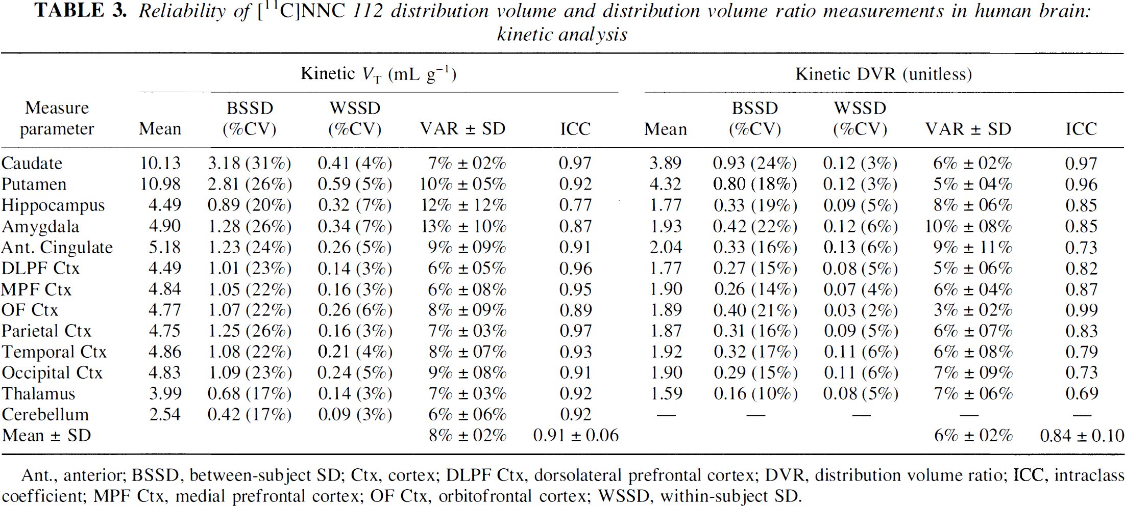
Ant., anterior; BSSD, between-subject SD; Ctx, cortex; DLPF Ctx, dorsolateral prefrontal cortex; DVR, distribution volume ratio; ICC, intraclass coefficient; MPF Ctx, medial prefrontal cortex; OF Ctx, orbitofrontal cortex; WSSD, within-subject SD.

OPEN IN VIEWER

TABLE 4.

Reliability of [¹¹C]NNC 112 BP and k₃/k₄ measurements in human brain: kinetic analysis

	Kinetic BP (mL g−1)					Kinetic k3/k4 (unitless)
Measure parameter	Mean	BSSD (%CV)	WSSD (%CV)	VAR ± SD	ICC	Mean	BSSD (%CV)	WSSD (%CV)	VAR ± SD	ICC
Caudate	7.51	2.98 (40%)	0.34 (5%)	8% ± 03%	0.97	2.89	0.93 (32%)	0.12 (4%)	8% ± 02%	0.97
Putamen	8.44	2.57 (30%)	0.51 (6%)	11% ± 05%	0.92	3.32	0.80 (24%)	0.12 (4%)	6% ± 05%	0.96
Hippocampus	1.92	0.77 (40%)	0.24 (13%)	18% ± 19%	0.82	0.77	0.33 (43%)	0.09 (12%)	18% ± 13%	0.85
Amygdala	2.35	1.12 (48%)	0.31 (13%)	23% ± 17%	0.86	0.93	0.42 (45%)	0.12 (13%)	21% ± 17%	0.85
Ant. Cingulate	2.64	0.98 (37%)	0.26 (10%)	19% ± 24%	0.87	1.04	0.33 (32%)	0.13 (13%)	20% ± 25%	0.73
DLPF Ctx	1.95	0.75 (39%)	0.14 (7%)	9% ± 08%	0.93	0.77	0.27 (35%)	0.08 (11%)	12% ± 11%	0.82
MPF Ctx	2.30	0.77 (34%)	0.12 (5%)	12% ± 10%	0.95	0.90	0.26 (29%)	0.07 (7%)	12% ± 08%	0.87
OF Ctx	2.21	0.97 (44%)	0.16 (7%)	11% ± 10%	0.95	0.89	0.40 (45%)	0.03 (4%)	7% ± 04%	0.99
Parietal Ctx	2.23	0.93 (42%)	0.17 (7%)	13% ± 09%	0.94	0.87	0.31 (35%)	0.09 (11%)	14% ± 12%	0.83
Temporal Ctx	2.32	0.87 (37%)	0.21 (9%)	13% ± 10%	0.89	0.92	0.32 (35%)	0.11 (12%)	11% ± 14%	0.79
Occipital Ctx	2.29	0.84 (37%)	0.23 (10%)	17% ± 12%	0.86	0.90	0.29 (32%)	0.11 (13%)	14% ± 15%	0.73
Thalamus	1.45	0.41 (28%)	0.15 (10%)	16% ± 08%	0.78	0.59	0.16 (27%)	0.08 (13%)	18% ± 12%	0.63
Mean ± SD				14% ± 05%	0.90 ± 0.06				13% ± 05%	0.84 ± 0.11

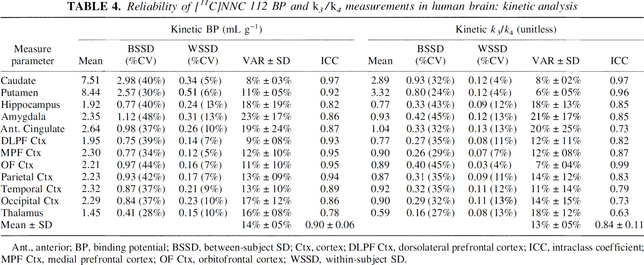
Ant., anterior; BP, binding potential; BSSD, between-subject SD; Ctx, cortex; DLPF Ctx, dorsolateral prefrontal cortex; ICC, intraclass coefficient; MPF Ctx, medial prefrontal cortex; OF Ctx, orbitofrontal cortex; WSSD, within-subject SD.

OPEN IN VIEWER

FIG. 9.

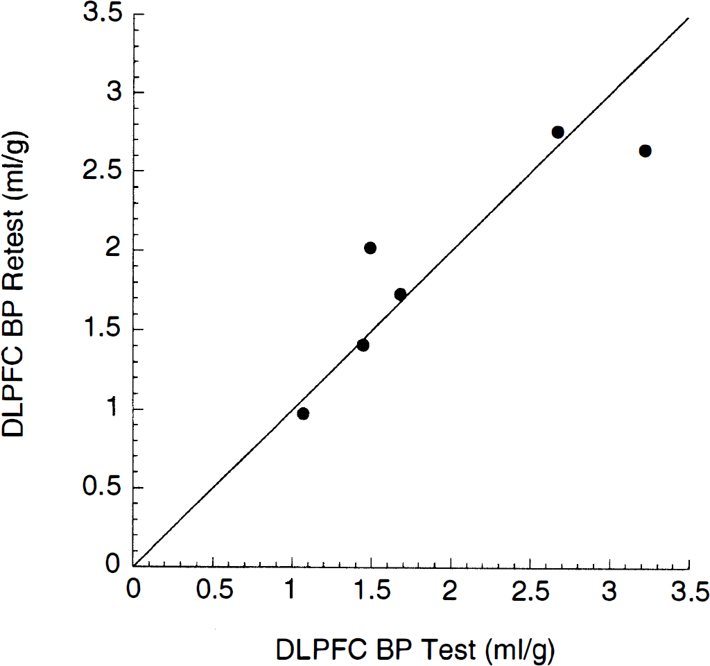
Relationship between [¹¹C]NNC 112 binding potential (BP) in dorsolateral prefrontal cortex in test (x axis) and retest (y axis) conditions. The solid line represents the line of identity. Linear regression of measured values had an r² of 0.82, corresponding to an intraclass coefficient of 0.93.

Graphical analysis

By visual inspection, Logan plots achieved linearity at times of >25 minutes, and a linear regression was performed on data from the 30- to 120-minute interval (Fig. 10). The V_T, BP, DVR, and k₃/k₄ values derived from graphical analysis are listed in Table 5. Regional V_T derivedby the graphical method was highly correlated with V_T derived by the kinetic method (r² = 0.99, P < 0.001, n = 144) but across regions was slightly lower by an average of 7 ± 3% (repeated-measures analysis of variance, P < 0.001). Regional DVR, BP, and k₃/k₄ values derived by graphical method were also highly correlated with values derived with kinetic method (r² = 0.99, P < 0.001) but were significantly lower, by averages of 14 ± 3, 23 ± 0.10, and 28 ± 9%, for DVR, BP, and k₃/k₄, respectively.

OPEN IN VIEWER

TABLE 5.

Graphical analysis of regional [¹¹C]NNC 112 uptake in human brain

Region	VT (mL g−1)	BP (mL g−1)	DVR (unitless)	k3/k4 (unitless)
Caudate	9.20 ± 3.25	6.45 ± 3.03	3.34 ± 0.91	2.34 ± 0.91
Putamen	10.57 ± 2.92	7.82 ± 2.65	3.84 ± 0.77	2.84 ± 0.77
Hippocampus	3.85 ± 0.78	1.15 ± 0.47	1.41 ± 0.22	0.43 ± 0.18
Amygdala	4.51 ± 1.18	1.75 ± 0.97	1.65 ± 0.34	0.65 ± 0.34
Ant. Cingulate	4.94 ± 1.22	2.19 ± 0.92	1.80 ± 0.28	0.80 ± 0.28
DLPF Ctx	4.19 ± 1.01	1.43 ± 0.72	1.52 ± 0.24	0.52 ± 0.24
MPF Ctx	4.59 ± 1.06	1.84 ± 0.73	1.67 ± 0.22	0.67 ± 0.22
OF Ctx	4.38 ± 1.22	1.71 ± 1.05	1.61 ± 0.41	0.67 ± 0.38
Parietal Ctx	4.43 ± 1.32	1.75 ± 0.84	1.59 ± 0.30	0.63 ± 0.25
Temporal Ctx	4.66 ± 1.09	1.90 ± 0.84	1.70 ± 0.28	0.70 ± 0.28
Occipital Ctx	4.62 ± 1.13	1.86 ± 0.84	1.68 ± 0.26	0.68 ± 0.26
Thalamus	3.56 ± 0.81	0.84 ± 0.48	1.30 ± 0.19	0.31 ± 0.17
Cerebellum	2.75 ± 0.48	—	—	—

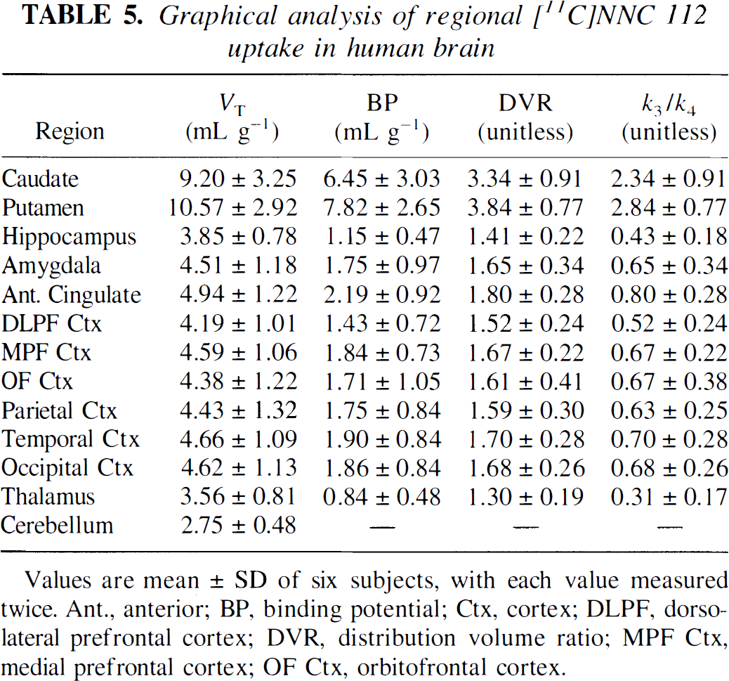
Values are mean ± SD of six subjects, with each value measured twice. Ant., anterior; BP, binding potential; Ctx, cortex; DLPF, dorsolateral prefrontal cortex; DVR, distribution volume ratio; MPF Ctx, medial prefrontal cortex; OF Ctx, orbitofrontal cortex.

OPEN IN VIEWER

FIG. 10.

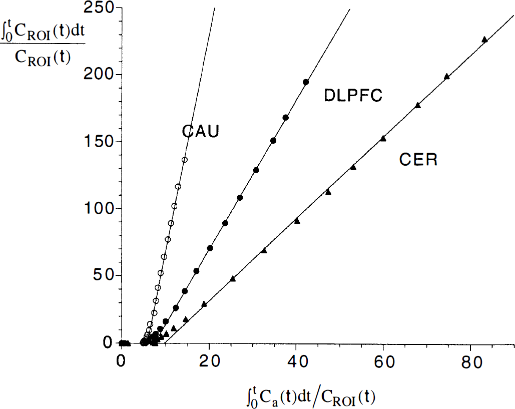
Graphical analysis of [¹¹C]NNC 112 uptake in caudate (open circles), dorsolateral prefrontal cortex (filled circles), and cerebellum (triangles) after injection of 18 mCi of [¹¹C]NNC 112 (same experiment as in Fig. 6). The linearity of the relationship at normalized times of >15 min (equal to 25 minutes of real time) confirms the reversibility of the binding.

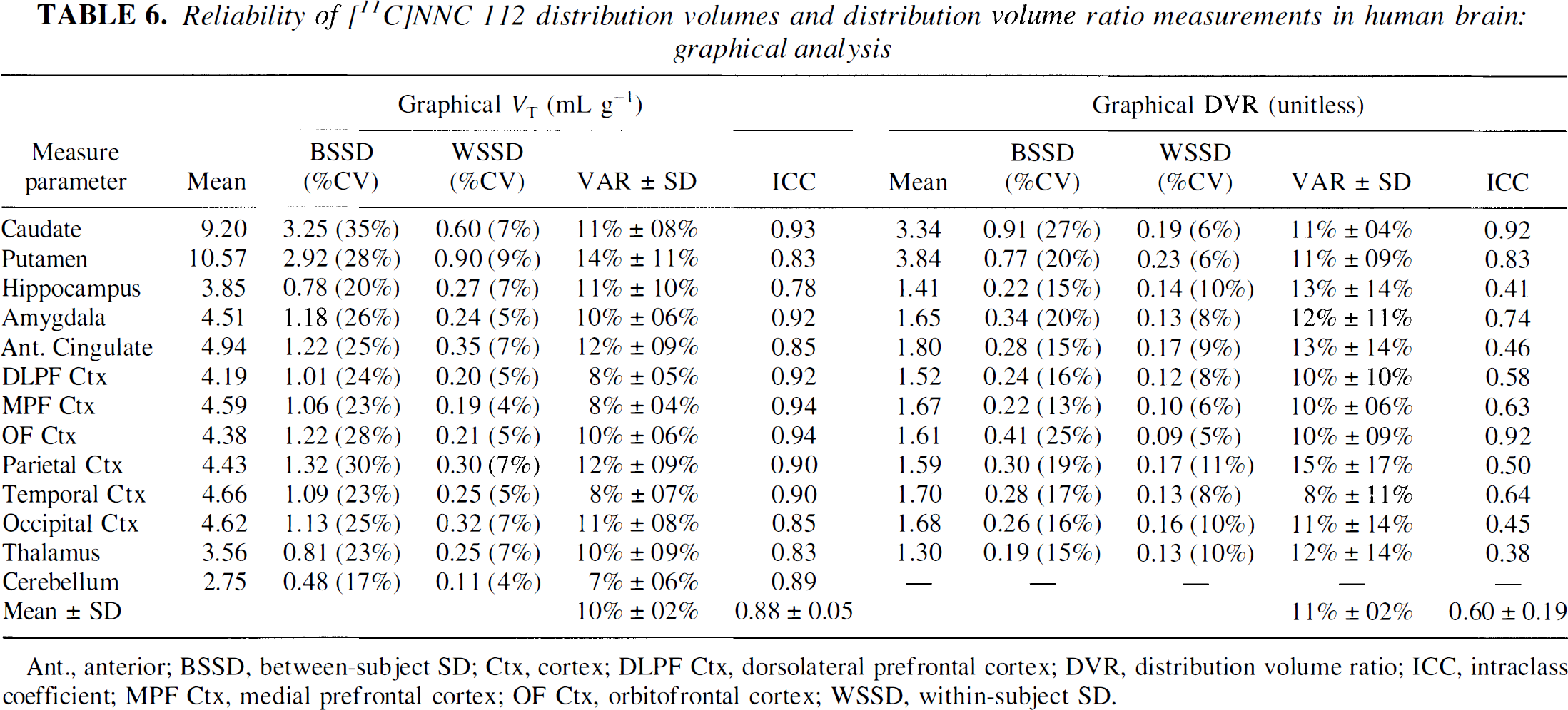
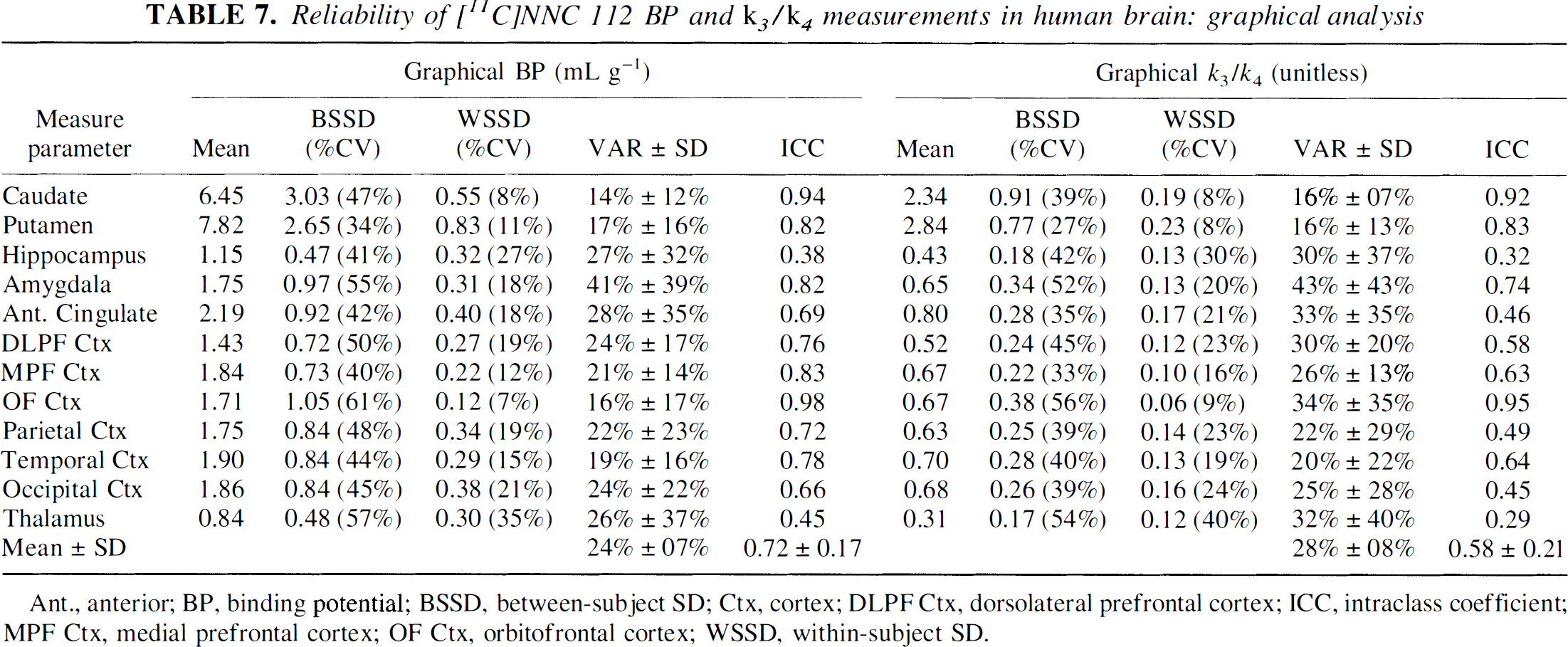
Tables 6 and 7 display the reproducibility parameters of the graphical method. As observed for kinetic analysis, the test/retest variability of V_T (10 ± 2%) and DVR (11 ± 2%) were lower than that of BP (24 ± 7%) and k₃/k₄ (28 ± 8%). The reliability of the absolute measures (V_T ICC = 0.88 ± 0.05, BP ICC = 0.72 ± 0.17) was superior to the reliability of the relative measures (DVR ICC = 0.60 ± 0.19, k₃/k₄ ICC = 0.58 ± 0.21). The test/retest variability of all outcome measures derived with graphical analysis was higher than results of kinetic analysis (e.g., graphical BP variability = 24 ± 7%, kinetic BP variability = 14 ± 5%, paired t test, P < 0.001). As a consequence, the reliability of outcome measures derived with graphical analysis was lower than with the kinetic analysis (e.g., graphical BP ICC = 0.72 ± 0.17, kinetic BP ICC = 0.90 ± 0.06, paired t test, P < 0.001).

OPEN IN VIEWER

TABLE 6.

Reliability of [¹¹C]NNC 112 distribution volumes and distribution volume ratio measurements in human brain: graphical analysis

	Graphical VT (mL g−1)					Graphical DVR (unitless)
Measure parameter	Mean	BSSD (%CV)	WSSD (%CV)	VAR ± SD	ICC	Mean	BSSD (%CV)	WSSD (%CV)	VAR ± SD	ICC
Caudate	9.20	3.25 (35%)	0.60 (7%)	11% ± 08%	0.93	3.34	0.91 (27%)	0.19 (6%)	11% ± 04%	0.92
Putamen	10.57	2.92 (28%)	0.90 (9%)	14% ± 11%	0.83	3.84	0.77 (20%)	0.23 (6%)	11% ± 09%	0.83
Hippocampus	3.85	0.78 (20%)	0.27 (7%)	11% ± 10%	0.78	1.41	0.22 (15%)	0.14 (10%)	13% ± 14%	0.41
Amygdala	4.51	1.18 (26%)	0.24 (5%)	10% ± 06%	0.92	1.65	0.34 (20%)	0.13 (8%)	12% ± 11%	0.74
Ant. Cingulate	4.94	1.22 (25%)	0.35 (7%)	12% ± 09%	0.85	1.80	0.28 (15%)	0.17 (9%)	13% ± 14%	0.46
DLPF Ctx	4.19	1.01 (24%)	0.20 (5%)	8% ± 05%	0.92	1.52	0.24 (16%)	0.12 (8%)	10% ± 10%	0.58
MPF Ctx	4.59	1.06 (23%)	0.19 (4%)	8% ± 04%	0.94	1.67	0.22 (13%)	0.10 (6%)	10% ± 06%	0.63
OF Ctx	4.38	1.22 (28%)	0.21 (5%)	10% ± 06%	0.94	1.61	0.41 (25%)	0.09 (5%)	10% ± 09%	0.92
Parietal Ctx	4.43	1.32 (30%)	0.30 (7%)	12% ± 09%	0.90	1.59	0.30 (19%)	0.17 (11%)	15% ± 17%	0.50
Temporal Ctx	4.66	1.09 (23%)	0.25 (5%)	8% ± 07%	0.90	1.70	0.28 (17%)	0.13 (8%)	8% ± 11%	0.64
Occipital Ctx	4.62	1.13 (25%)	0.32 (7%)	11% ± 08%	0.85	1.68	0.26 (16%)	0.16 (10%)	11% ± 14%	0.45
Thalamus	3.56	0.81 (23%)	0.25 (7%)	10% ± 09%	0.83	1.30	0.19 (15%)	0.13 (10%)	12% ± 14%	0.38
Cerebellum	2.75	0.48 (17%)	0.11 (4%)	7% ± 06%	0.89	—	—	—	—	—
Mean ± SD				10% ± 02%	0.88 ± 0.05				11% ± 02%	0.60 ± 0.19

Ant., anterior; BSSD, between-subject SD; Ctx, cortex; DLPF Ctx, dorsolateral prefrontal cortex; DVR, distribution volume ratio; ICC, intraclass coefficient; MPF Ctx, medial prefrontal cortex; OF Ctx, orbitofrontal cortex; WSSD, within-subject SD.

OPEN IN VIEWER

TABLE 7.

Reliability of [¹¹C]NNC 112 BP and k₃/k₄ measurements in human brain: graphical analysis

	Graphical BP (mL g−1)					Graphical k3/k4 (unitless)
Measure parameter	Mean	BSSD (%CV)	WSSD (%CV)	VAR ± SD	ICC	Mean	BSSD (%CV)	WSSD (%CV)	VAR ± SD	ICC
Caudate	6.45	3.03 (47%)	0.55 (8%)	14% ± 12%	0.94	2.34	0.91 (39%)	0.19 (8%)	16% ± 07%	0.92
Putamen	7.82	2.65 (34%)	0.83 (11%)	17% ± 16%	0.82	2.84	0.77 (27%)	0.23 (8%)	16% ± 13%	0.83
Hippocampus	1.15	0.47 (41%)	0.32 (27%)	27% ± 32%	0.38	0.43	0.18 (42%)	0.13 (30%)	30% ± 37%	0.32
Amygdala	1.75	0.97 (55%)	0.31 (18%)	41% ± 39%	0.82	0.65	0.34 (52%)	0.13 (20%)	43% ± 43%	0.74
Ant. Cingulate	2.19	0.92 (42%)	0.40 (18%)	28% ± 35%	0.69	0.80	0.28 (35%)	0.17 (21%)	33% ± 35%	0.46
DLPF Ctx	1.43	0.72 (50%)	0.27 (19%)	24% ± 17%	0.76	0.52	0.24 (45%)	0.12 (23%)	30% ± 20%	0.58
MPF Ctx	1.84	0.73 (40%)	0.22 (12%)	21% ± 14%	0.83	0.67	0.22 (33%)	0.10 (16%)	26% ± 13%	0.63
OF Ctx	1.71	1.05 (61%)	0.12 (7%)	16% ± 17%	0.98	0.67	0.38 (56%)	0.06 (9%)	34% ± 35%	0.95
Parietal Ctx	1.75	0.84 (48%)	0.34 (19%)	22% ± 23%	0.72	0.63	0.25 (39%)	0.14 (23%)	22% ± 29%	0.49
Temporal Ctx	1.90	0.84 (44%)	0.29 (15%)	19% ± 16%	0.78	0.70	0.28 (40%)	0.13 (19%)	20% ± 22%	0.64
Occipital Ctx	1.86	0.84 (45%)	0.38 (21%)	24% ± 22%	0.66	0.68	0.26 (39%)	0.16 (24%)	25% ± 28%	0.45
Thalamus	0.84	0.48 (57%)	0.30 (35%)	26% ± 37%	0.45	0.31	0.17 (54%)	0.12 (40%)	32% ± 40%	0.29
Mean ± SD				24% ± 07%	0.72 ± 0.17				28% ± 08%	0.58 ± 0.21

Ant., anterior; BP, binding potential; BSSD, between-subject SD; Ctx, cortex; DLPF Ctx, dorsolateral prefrontal cortex; ICC, intraclass coefficient; MPF Ctx, medial prefrontal cortex; OF Ctx, orbitofrontal cortex; WSSD, within-subject SD.

Noise analysis

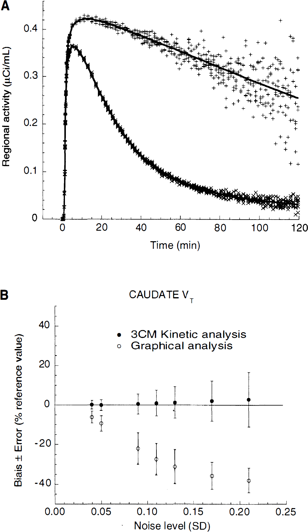
Noise analysis was done to compare the effect of realistic noise in the images on results from the kinetic and graphical analyses (Fig. 11). A typical experiment was used to generate a simulated data set that included one cerebellar curve (two-compartment model, K₁ = 0.120 mL g⁻¹ min⁻¹, k₂ = 0.0526 min⁻¹, V_T = 2.28 mL g⁻¹) and one caudate curve (three-compartment model, K₁ = 0.130 mL g⁻¹ min⁻¹, k₂ = 0.0570 min⁻¹, k₃ = 0.110 min⁻¹, k₄ = 0.034 min⁻¹, V_T = 9.65 mL g⁻¹, BP = 7.38 mL g⁻¹, k₃/k₄ = 3.24). Random noise was then introduced as described in Materials and Methods, and noisy data sets were analyzed with kinetic and graphical analyses. Seven noise levels were investigated (SD_J of 0.04, 0.05, 0.09, 0.11, 0.13, 0.17, and 0.21), and for each noise level, 500 curves were created and analyzed. For each region and noise level, Table 8 lists the average ±SD V_T values derived with the 500 simulations, the bias (i.e., difference between average of 500 simulations and true V_T), and the error (%CV of the 500 simulations).

OPEN IN VIEWER

TABLE 8.

Noise analysis of cerebellum and caudate: comparison of kinetic and graphical methods

	Cerebellum
	Kinetic analysis (2CM)			Graphical analysis
Region noise level (SDJ)	VT ± SD	Bias	Error	VT ± SD	Bias	Error
0	2.3085			2.2156	—	—
0.04	2.3086 ± 0.0031	0.00%	0.13%	2.2078 ± 0.0073	−0.35%	0.33%
0.05*	2.3083 ± 0.0038	−0.01%	0.16%	2.2031 ± 0.0099	−0.56%	0.45%
0.09	2.3087 ± 0.0069	0.01%	0.30%	2.1723 ± 0.0250	−1.95%	1.15%
0.11	2.3088 ± 0.0085	0.01%	0.37%	2.1561 ± 0.0291	−2.69%	1.35%
0.13	2.3084 ± 0.0098	0.00%	0.42%	2.1405 ± 0.0332	−3.39%	1.55%
0.17	2.3091 ± 0.0131	0.03%	0.57%	2.1178 ± 0.0316	−4.41%	1.49%
0.21	2.3075 ± 0.0166	−0.04%	0.72%	2.1093 ± 0.0321	−4.80%	1.52%
	Caudate
	Kinetic analysis (3CMcst)			Graphical analysis
0	9.6594	—	—	9.6216	—	—
0.04	9.6726 ± 0.2129	0.14%	2.20%	9.0261 ± 0.2679	−6.19%	2.97%
0.05*	9.6575 ± 0.2637	−0.02%	2.73%	8.7161 ± 0.3426	−9.41%	3.93%
0.09	9.7159 ± 0.4899	0.58%	5.04%	7.4942 ± 0.5946	−22.11%	7.93%
0.11	9.7549 ± 0.6340	0.99%	6.50%	6.9921 ± 0.5585	−27.33%	7.99%
0.13	9.7813 ± 0.7817	1.26%	7.99%	6.6233 ± 0.5671	−31.16%	8.56%
0.17	9.8543 ± 1.0004	2.02%	10.15%	6.1875 ± 0.4183	−35.69%	6.76%
0.21	9.9252 ± 1.3677	2.75%	13.78%	5.9661 ± 0.3705	−37.99%	6.21%

*

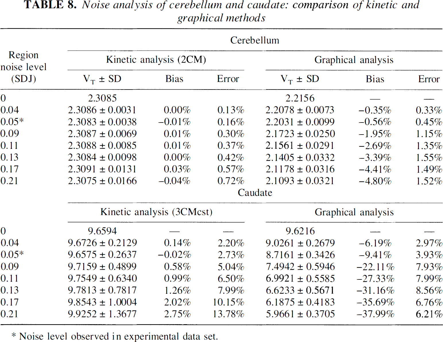
Noise level observed in experimental data set.

OPEN IN VIEWER

FIG. 11.

Noise analysis. (A) Simulated time-activity data in caudate and cerebellum. The solid line represents a simulated noise-free brain response to a typical input function with a typical set of kinetic parameters. Crosses correspond to 10 simulated brain responses with random noise. Noise had 0 mean and a SD (SD_J) of 0.09. The noise increases with the duration of the experiment to reflect the decay of ¹¹C. (B) Results of analysis of caudate data sets with random noise, at different noise levels corresponding to SN_J ranging from low (0.04) to high noise (0.21). At each level, 10 curves were generated and analyzed with kinetic and graphical analyses. Values correspond to the mean V_T values of these 10 analyses, expressed as relative difference from the true value used to generate the simulation. The vertical bar is the SD of the result from the 10 simulations. For kinetic analysis, no significant bias is observed; that is, the mean of 10 simulations is close to the true value. In contrast, graphical analysis is affected by a noise-dependent bias. As the noise increases, the mean V_T value derived from the 10 simulations becomes lower than the true value. The SD of the 10 V_T values increased as the noise level increased similarly for kinetic and graphical analyses.

Both analyses were very robust as far as the cerebellum was concerned. For cerebellar kinetic analysis, the bias was negligible, and the error was very small (both bias and error < 1%). Cerebellar graphical analysis showed higher bias and errors than the kinetic analysis but remained within acceptable levels at each noise level.

Analysis of caudate curves was more sensitive to noise. Kinetic analysis showed a small bias (+2.7% at higher noise level), and the error increased to ±14% at the highest noise level. Graphical analysis was characterized by a pronounced bias. As noise increased, graphical V_T significantly decreased, up to −38% at the highest noise level. The error on graphical V_T was comparable with that on the kinetic V_T, except that kinetic errors were larger than graphical errors at the two highest noise levels. The bias associated with graphical analysis (lower value as noise increases) was consistent with the results obtained on the experimental data set.

Comparison with [¹¹C]SCH 23390

Results of this study indicate that [¹¹C]NNC 112 achieves higher specific/nonspecific DVRs at equilibrium than [¹¹C]SCH 23390. In the putamen, [¹¹C]SCH 23390 k₃/k₄ value derived by graphical analysis was 0.85 ± 0.18 (Chan et al., 1998), lower than the value reported here with [¹¹C]NNC 112 in the same region (3.32 ± 0.80). In the PFC, Okubo et al. (1997) reported an [¹¹C]SCH 23390 k₃/k₄ value of 0.41 ± 0.06, lower than the k₃/k₄ value observed with [¹¹C]NNC 112 in the DLPFC (0.77 ± 0.33). This improvement is due not only to the higher affinity of [¹¹C]NNC 112 (K _D = 0.18 nmol/L; Andersen et al., 1992) compared with [¹¹C]SCH 23390 (0.4 nmol/L; Billard et al., 1984) but also to lower nonspecific binding. Cerebellar V_T is 2.54 ± 0.42 mL g⁻¹ for [¹¹C]NNC 112 versus 3.58 ± 0.64 mL g⁻¹ for [¹¹C]SCH 23390 (Chan et al., 1998). This higher signal/noise ratio is especially valuable for quantification of D₁ receptors in the neocortex.

Neocortical region-of-interest sampling

In this study, an original method was developed for sampling of activity in neocortical regions. Measurement of activity in large subcortical regions such as the striatum is generally straightforward, inasmuch as the boundaries of activity can be well defined anatomically. In the striatum, MRI-guided ROI definition does not substantially improve the reliability of the measurement compared with direct definition of the ROI on the PET image based on activity distribution (Wang et al., 1996). In contrast, measurement of activity distribution in GM cortical areas is a difficult problem due to the extent and complexity of cortical gray geometry (see discussion in Koepp et al., 1997). The simplest method is to draw geometrically simple structures (spheres, rectangles) directly on the PET scan, but this method is unreliable and influenced by the activity distribution on the PET image. Thus, defining the ROI on a coregistered MR image is preferable. However, tracing contours of a cortical region manually around the GM on high-resolution 128-slice MRI is time consuming and subject to rater bias and errors. In this study, we used a method based on coregistration of the PET data set to a segmented MRI data set, that is, a data set in which each pixel has been designated as GM, WM, or CSF value. Only the activity located in the pixels classified as GM is sampled. The advantage of constraining ROI on GM is that the segmentation procedure is operator independent and much faster and reliable than manual tracing of GM/WM/CSF boundaries. The only operator-driven choice is the choice of the limits between cortical regions, which follows well-defined criteria. The excellent reliability of the cortical measurement of [¹¹C]NNC 112 BP reported in this study indirectly supports the robustness of the method.

It is, however, important to keep in mind that this method has several limitations. Like all MRI-based ROI definitions, this method is sensitive to errors in PET-MRI coregistration. In this study, we used the minimization procedure developed by Woods et al. (1993). This procedure has a reported average three-dimensional error of <2 mm for between-modality registration, which is acceptable, given a camera resolution of 6 mm. Second, this sampling method results in inherent subsampling, inasmuch as the activity spilling over the WM is not measured. This subsampling is desirable from an accuracy point of view but results in a loss of information that might translate into increased noise. Finally, this method does not correct for partial voluming, which is considerable in the cortex. Yet, it provides a necessary first step for implementation of ROI-based partial volume correction (Rousset et al., 1998). In fact, partial volume correction would result in a recovery of the spilled-over information. Thus, partial volume correction has the potential not only to increase the accuracy of the measurement but also to reduce the error by using the information that is rejected in the present method. We are currently developing and testing a partial volume correction method that would address these issues.

Evaluation of kinetic approach

Evaluation of model-based methods for quantification of receptor parameters includes assessment of various criteria, namely, identifiability, validity, stability, and reliability. The identifiability is a mathematical dimension referring to the confidence in the value of the parameter as derived by the fitting process. The validity refers to the physiological plausibility of the parameters and is usually determined in relationship to in vitro results. The stability refers to the independence of the parameter estimate from the amount of data collected, in this case the duration of the experiment. The reliability expresses the test/retest variability in relation to between-subject differences. Kinetic analysis of [¹¹C]NNC 112 regional uptake performed well on all of these criteria.

Kinetic analysis of the cerebellum presented an interesting problem. The three-compartment model provided a slightly but significantly superior fit to the data compared with the two-compartment model. The observation of a better fit by the three- compared with the two-compartment model for a region of a reference is the rule rather than the exception in neuroreceptor imaging (Frost et al., 1989; Logan et al., 1990; Laruelle et al., 1994b, 1994c; Lammertsma et al., 1996; Abi-Dargham et al., 1997; Ito et al., 1998). The absence of specific binding in the cerebellum is confirmed by the absence of displacement of [¹¹C]NNC 112 uptake in the cerebellum after injection of SCH 23390 (2.5 mg/kg) (Halldin et al., 1998). Thus, the small second tissue compartment revealed by the three-compartment model's superior fit might reflect a slow buildup of radiolabeled metabolites in the brain or the existence of a nonspecific binding component with slow kinetics. The presence of a statistically superior fit with the three-compartment model would usually suggest the use of a three-compartment model to derive cerebellar V_T. However, in this case, V_T derived by the three-compartment model was less well identified than with a two-compartment model, was markedly affected by the duration of the scan, had a poor test/retest reproducibility (negative ICC), and provided values much larger than the value of V_T derived by the graphical analysis. Thus, whereas the goodness of fit favored the three-compartment model, all other criteria favored the two-compartment model. For these reasons, we favored the two-compartment model, that is, the solution that provides superior identifiability, stability, validity, and reproducibility.

For ROIs, we used a three-compartment model with K₁/k₂ ratio constrained to the value of V_T measured in the cerebellum. Whereas an unconstrained three-compartment model is usually appropriate to derive V_T, the separate derivation of V₂ and BP is not reliable with an unconstrained three-compartment model (Laruelle et al., 1994d, 1994e; Lammertsma et al., 1996). The constrained approach takes advantage of the knowledge of V₂ derived from the region of reference while accommodating regional differences in blood flow. The validity of this approach is supported by the homogeneous distribution of the inactive enantiomer (−)[¹¹C]NNC 112 within the human and baboon brain (Halldin et al., 1998). The goodness of fit was excellent, with even distribution of the residuals, and regional distribution volumes were well identified.

A significant relationship was observed between regional BP and regional density of D₁ receptor measured in vitro in the human brain (Table 2). Yet, subtle differences were observed. In vitro, D₁ receptor density is slightly higher in caudate than putamen, whereas the reverse is true in the PET measurements. In vitro, D₁ receptor density is higher in the amygdala than hippocampus, but this difference is less pronounced in the PET measurements. In vitro, frontal D₁ receptor density is higher than occipital D₁ receptor density, but PET measurements gave similar BP. These differences can be accounted for by partial volume effects, resulting in relative underestimation of smaller regions versus larger regions (caudate versus putamen, amygdala versus hippocampus, frontal GM versus occipital GM).

Results of kinetic modeling were essentially stable from 90 minutes to the end of the experiment. The stability over time of the solution means that the model describes the data appropriately and that enough data were collected to inform the model. Remarkably, this was true for both striatal and extrastriatal areas. It is often difficult to accurately measure receptor parameters with the same radiotracer both in regions with high and low receptor densities. High affinity is required for a high signal/noise ratio in regions with low receptor density, but high affinity might preclude favorable kinetics in regions with high receptor density. [¹¹C]NNC 112 achieves an effective balance between these competing requirements. However, 90 minutes of data was needed to achieve stability of the outcome measure. The three-dimensional acquisition mode, with its higher sensitivity, is crucial to enable data collection up to 120 minutes. The use of the polyurethane head mold was effective, as only minimal head movement was recorded during this prolonged time frame. Head movement was measured by comparing the spatial location of the ¹¹C markers on each frame and was <2.5 mm per frame in ∼90% of the cases. Thus, the combination of the high sensitivity of the three-dimensional mode and the effective headholder allowed collection of enough data to achieve stability of the results.

Reproducibility and outcome measures

Several statistical parameters and outcome measures are used in the PET/single photon emission computed tomography neuroreceptor literature to report the reproducibility of the measurements. The most straightforward reproducibility parameter is the absolute test/retest variability, calculated as the absolute difference between test and retest values divided by their average (Abi-Dargham et al., 1995; Seibyl et al., 1995; Smith et al., 1998). A second method consists of reporting the within-subject SD (or %CV) of the measurement (Chan et al., 1998). When the number of repeat scans is 2, the within-subject %CV is smaller than the variability by a factor of 2^1/2. Finally, the ICC provides a measure of the reproducibility of the measurement relative to between-subject differences and is the most useful measure to compare results of various methods.

In this study, four outcome measures (V_T, DVR, BP, and k₃/k₄) were compared in terms of reproducibility and reliability. These commonly used outcome measures in the PET literature have very different relationships vis à vis receptor B_max and K_D. In essence, V_T and BP are “absolute” measures that relate brain distribution volumes to the input function and are expressed as milliliters (of plasma) over grams (of tissue). V_T is the total distribution volume, including free, nonspecific, and specific binding. The use of V_T as outcome measure should be restricted to situations when nonspecific binding cannot be measured for a lack of region of reference and is negligible compared with the specific binding, such as in the case of [¹¹C]flumazenil (Koeppe et al., 1991) or [¹²³I]iomazenil (Abi-Dargham et al., 1994). Otherwise, BP is the outcome measure of choice because it is directly equal to the B_max/K_D ratio and does not include nonspecific binding. The reproducibility of V_T is intrinsically superior to BP, as BP is derived by the difference between two V_T measurements (V_T of the ROI and V_T of the region of reference), and this is especially true in regions with low BP relative to V₂. In this study, the test/retest variability of V_T (8 ± 2%) was better than the variability of BP (14 ± 5%).

In contrast to V_T and BP, DVR and k₃/k₄ are “relative” outcome measures in the sense that they represent distribution volumes “normalized” by the region of reference, in this case the cerebellum. Both outcome measures are related (DVR − 1 = k₃/k₄), yet only k₃/k₄ expresses a meaningful quantity. Although both outcome measures are linearly related to BP, the relationship between DVR and BP has an intercept of 1, meaning that DVR assumes a value of 1 in a region with BP = 0. Thus, DVR is inappropriate to express receptor density. However, studies reporting reproducibility of neuroreceptor measurements frequently report DVR instead of k₃/k₄ (Volkow et al., 1993; Chan et al., 1998; Smith et al., 1998). The reproducibility of DVR is intrinsically better than the reproducibility of k₃/k₄, and this is especially true in regions with low receptor density. In this study, the test/retest variabilities of DVR and k₃/k₄ were 6 ± 2 and 13 ± 5%, respectively. The DVR variability observed in this study (6%) is in the same range as the variability of DVR for [¹¹C]raclopride in the striatum (5%) (Volkow et al., 1993), [¹¹C]SCH 23390 in the striatum (within-subject %CV of 3%) (Chan et al., 1998), and [¹⁸F]altanserin in cortical regions (ranging from 7 to 9%, n = 8) (Smith et al., 1998).

BP versus k₃/k₄

As a region of reference can be measured for [¹¹C]NNC 112 (i.e., cerebellum), the only meaningful choices of outcome measures for clinical studies are either BP or k₃/k₄. Usually, the reproducibility of k₃/k₄ is better than BP because the data are normalized by cerebellum V_T and k₃/k₄ is less sensitive to errors associated with plasma input function measurement and cross-calibration between PET camera and well counter. However, in this study, the average test/retest variability of BP (14 ± 5%) was similar to that of k₃/k₄ (13 ± 5%), and the reliability of BP (ICC = 0.90 ± 0.06) was slightly better than that of k₃/k₄ (0.84 ± 0.11). Thus, according to these data, both outcome measures essentially perform similarly, and the choice between the two depends on the inherent assumptions one is willing to accept.

The BP as expressed in Eq. 10 is the only expression of BP that is exclusively dependent on receptor parameters and unbiased by factors unrelated to receptors. However, in this study, BP was not corrected for f₁. The free fraction of [¹¹C]NNC 112 in plasma was low (1.02 ± 0.28% of total plasma concentration), and no between-subject differences in f₁ were reliably detected (f₁ ICC = −0.20). Thus, the within-subject %CV associated with f₁ measurement (±34%) was of the same magnitude as the between-subject %CV in f₁ (±27%). Under these conditions, individual f₁ values should not be used in the calculation of the distribution volumes (Abi-Dargham et al., 1995). Yet, the use of this uncorrected BP is associated with a potential bias introduced by between-subject differences in f₁. Although this study did not support the utility of this correction in healthy subjects, it may still be necessary to control for potential alterations of plasma protein binding in pathological conditions. On the other hand, the cost associated with the use of k₃/k₄ is the potential bias introduced by between-subject differences in nonspecific binding, which might lead to between-subject differences in k₃/k₄ that are unrelated to receptor parameters. True between-subject differences in nonspecific binding were demonstrated in this study (the between-subject %CV of cerebellum V_T was 17%). Thus, both the uncorrected BP used in this study and k₃/k₄ have potential pitfalls. Between-subject differences in plasma protein binding would bias BP but not k₃/k₄. Between-subject differences in nonspecific binding to brain tissue would bias k₃/k₄ but not BP. With these limitations in mind, the slightly better reliability of BP compared with k₃/k₄ suggests that BP should be the outcome measure of choice for between-subject comparison. Yet, this advantage might be offset by the convenience of measuring k₃/k₄ using the cerebellum as input function instead of the plasma (Ichise et al., 1996; Lammertsma et al., 1996; Logan et al., 1996). Additional analysis comparing the reliability of k₃/k₄ measurement with and without plasma input function is required to resolve this issue.

Kinetic versus graphical analysis

Distribution volumes derived by graphical and kinetic analyses were strongly correlated (r² = 0.99, P < 0.001), but results of graphical analysis resulted in lower values of V_T (by 7 ± 3%), BP (by 23 ± 10%), and k₃/k₄ (28 ± 9%). Differences between graphical and kinetic BP and k₃/k₄ can be partially accounted for by the fact that cerebellum V_T was higher with graphical than kinetic analysis, which might be linked to an underestimation of cerebellum V_T as derived by two-compartment model. However, these differences are also due to differences in ROI V_T. A systematic difference between kinetic and graphical V_T was an unexpected finding. Another unexpected difference was the lower reproducibility of graphical V_T (test/retest variability = 10 ± 2%, ICC = 0.88) compared with kinetic V_T (8 ± 2%, ICC = 0.91). The lower reproducibility of graphical compared with kinetic outcomes was even more accentuated for BP and k₃/k₄. This result undermines the claim that graphical analysis is less sensitive to noise and statistical fluctuation of the data than kinetic analysis (Volkow et al., 1993).

Analysis of the effect of noise on the outcome measure derived by both methods was performed to better understand this phenomenon. Realistic noisy data sets were generated in which the noise increased with the duration of the experiment proportionally to the decay of ¹¹C. The impact of the noise on the outcome measure was very different for kinetic and graphical analyses. As noise increased, both methods were associated with a similar variability, but V_T derived by kinetic analysis remained essentially unbiased, whereas the graphical analysis yielded systematically lower values. As the noise was randomly distributed around the true values with zero mean, the noise-introduced bias toward lower outcome measures in the graphical analysis was not intuitively predicted. This noise-dependent bias was introduced by the linearization process in which both predictor and response variables are subject to error. This phenomenon, observed here for the graphical analysis, is comparable with the noise-dependent bias introduced by the Scatchard transformation used in analysis of saturation binding data (Munson and Rodbard, 1980) and has been previously described (Carson, 1993).

At the highest noise level (SD_J = 0.21), this bias resulted in a 38% underestimation of V_T by graphical analysis (i.e., the mean of the 500 simulations was 38% lower than the true value used to generate the curves). Simulations performed on other regions such as the DLPFC yielded similar results (data not shown). We also observed that the noise-dependent bias was related to the slope of the regression (i.e., on the magnitude of V_T). Therefore, regions with lower receptor density were less vulnerable to this effect than regions with high receptor density (cerebellum < DLPFC < caudate). This slope dependency also contributed to the greater underestimation of BP and k₃/k₄ by graphical analysis compared with V_T, to the extent that regions with receptors were more affected than cerebellum.

A large range of noise was used to generate these simulations (SD_J from 0.04 to 0.21). To determine which level of noise corresponded to the experimental noise, we compared the mean sum of squares of the residuals as well as the identifiability (percent error) of V_T at each level of noise in the simulations with the mean sum of squares and percent error effectively observed in the experimental data set. The mean sum of squares observed in the caudate in the experimental data was 0.35 ± 0.21 nCi/mL (n = 12). The simulations with SD_J of 0.04 and 0.05 gave mean mean sums of squares of 0.25 and 0.39 nCi/mL, respectively. The percent error associated with V_T in the caudate in the experimental data was 2.6 ± 0.7% (n = 12). The simulations with SD_J of 0.05 and 0.09 had percent errors of 1.8 and 3.2%, respectively. Thus, the experimental mean sum of squares falls between SD_J of 0.04 and 0.05, and the experimental percent error falls between SD_J of 0.05 and 0.09. Therefore, the simulation with SD_J of 0.05 appears to provide a noise level comparable with the noise observed experimentally.

At this noise level, caudate kinetic analysis had no bias (−0.02%), but the graphical analysis had a significant bias (−9.41%). The bias associated with graphical analysis at this noise level might account for the lower V_T measured in the caudate with the graphical analysis (9.3 ± 3.6 mL g⁻¹) compared with the kinetic analysis (10.3 ± 3.6 mL g⁻¹). This difference was significant (repeated-measures analysis of variance, P = 0.007) and averaged −11 ± 7%. In addition, as the noise might vary from test to retest condition, this phenomenon might explain the lower reproducibility of the graphical method compared with the kinetic analysis. These results indicate that kinetic modeling is the method of choice for the derivation of D₁ receptor BP or k₃/k₄ with [¹¹C]NNC 112.