Maximizing Profit via Assortment and Shelf‐Space Optimization for Two‐Dimensional Shelves

Abstract

Product proliferation and changes in demand require that retailers regularly determine how items should be allocated to retail shelves. The existing shelf‐space literature mainly deals with regular retail shelves onto which customers only have a frontal perspective. This study provides a modeling and solution approach for two‐dimensional shelves, e.g., for meat, bread, fish, cheese, or clothes. These are categories that are kept on tilted shelves. Customers have a total perspective on these shelves and can observe units of one particular item horizontally and vertically instead of just seeing the foremost unit of an item, as is the case of regular shelves. We develop a decision model that optimizes the two‐dimensional shelf‐space assignment of items to a restricted, tilted shelf. We contribute to current literature by integrating the assortment decision and accounting for stochastic demand, space elasticity and substitution effects in the setting of such self types. To solve the model, we implement a specialized heuristic that is based on a genetic algorithm (GA). By comparing it to an exact approach and other benchmarks, we prove its efficiency and demonstrate that results are near‐optimal with an average solution quality of above 99% in terms of profit. Based on a numerical study with data from one of Germany’s largest retailers, we were able to show within the scope of a case study that our approach can lead to an increase in profits of up to 15%. We demonstrate with further simulated data that integration of stochastic demand, substitution, and space elasticity results in up to 80% higher profits.

Keywords

shelf‐space planning substitution space elasticity stochastic demand tilted shelf

Introduction

This study considers the problem of selecting, allocating and arranging products on retail shelves. Shelf space has been referred to as one of the retailer’s scarcest resources (cf. e.g., Brown and Tucker 1961, Geismar et al. 2015, Hübner et al. 2013a, Kök et al. 2015, Lim et al. 2004, Reiner et al. 2012). Up to 30% more products compete for the limited space than was the case ten years ago (EHI Retail Institute 2014, Hübner et al. 2016). The increasing number of items to allocate, the shortage of shelf space, narrow margins in retail and the intensity of competition have greatly magnified the importance of retail assortment and shelf‐space planning (cf. Hübner et al. 2013b). Furthermore, customer satisfaction is mostly driven by availability of the right products. In order to achieve superior performance, retailers have to recognize customers’ needs and identify these as key drivers (Eltze et al. 2013, Nielsen 2004).

The selection of items and space allocation of the items to the shelf are interdependent planning problems when shelf space is restricted. The space available per product is less if broader assortments are offered and vice versa. Consequently, planning retail shelves involves the tasks of specifying the product assortments as well determining the space and quantities for selected items. These decisions are not only based on the margins of the products but also on associated demand and customer preferences. The more shelf space is allocated to an item, the more it attracts customers and the higher its demand. This is referred to as “space‐elastic demand.” This topic has gained a lot of research attention over recent years (see e.g., Bianchi‐Aguiar et al. 2019, Hübner and Kuhn 2012, Kök et al. 2015). Common characteristics of these models are that demand depends on the number of facings (= the foremost unit of an item in the front row of the shelf), and that retail shelves are observed by customers from a frontal direction. This firstly implies that a customer can only see the facing, and secondly, that two different products can only be positioned next to but not behind one another. We refer to this shelf type as a “regular shelf” herein. For example, candies, coffee and tea, canned goods, cleaners, and personal care products are presented on regular shelves.

Not all retail categories are kept on regular shelves. Some products are presented on “tilted shelves” (like counters, fridges or tables) onto which customers have a total perspective. Examples of these shelf types are to be found in Figure 1. These two‐dimensional shelves types are, for example, used for the presentation of fresh food like bakery products and sausages, frozen products or in fashion retailing and consumer electronics. Many other retail formats fit into these settings, e.g., products and magazines in kiosks, snacks or electronics in vending machines and display ads (see also Geismar et al. 2015). With these shelves, items can be arranged more flexibly in the two‐dimensional space, whereas with regular shelves the options are restricted by the shelf levels and their height. For example, two different products can be positioned next to and behind one another on two‐dimensional shelves.

Figure 1

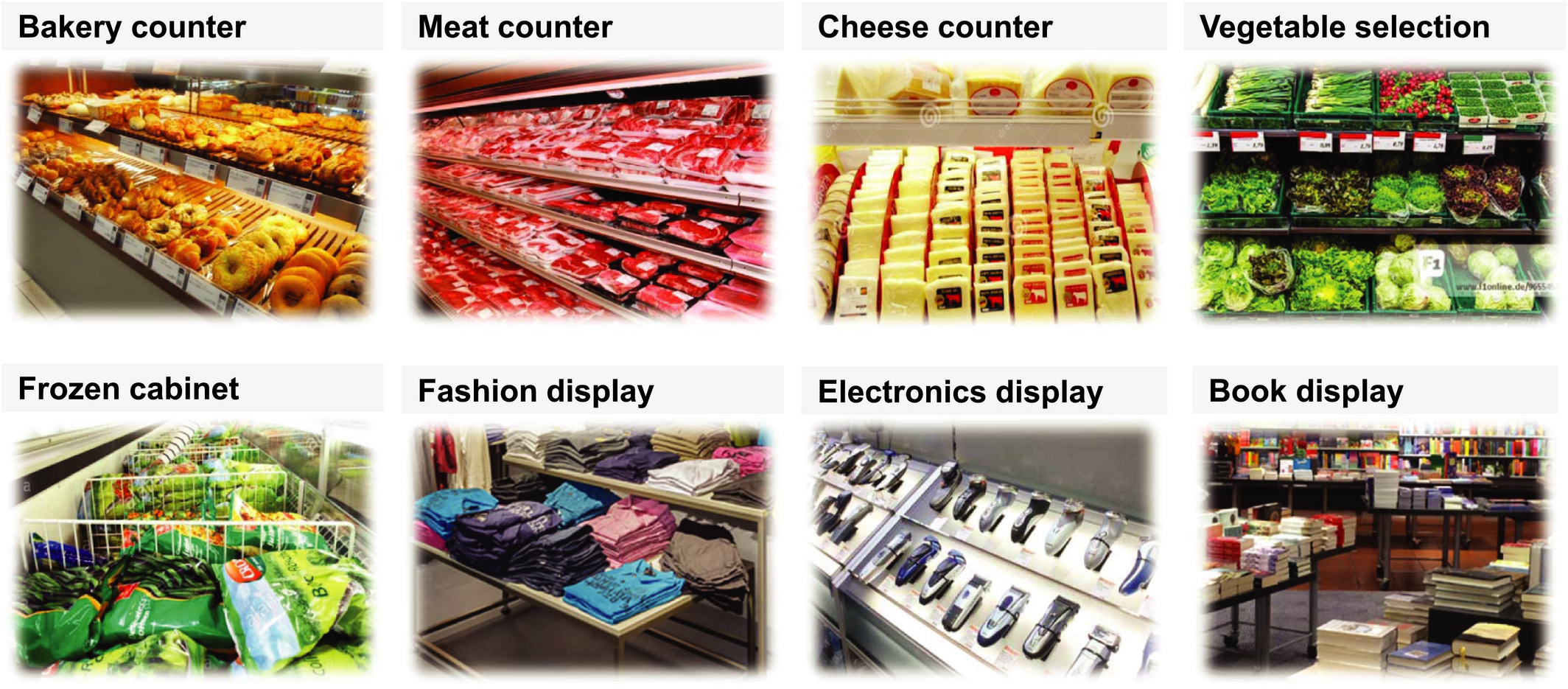
Examples of Categories Stored on Two‐Dimensional Shelves [Color figure can be viewed at wileyonlinelibrary.com]

There is already a rich literature on the planning of regular shelves. Typically, these models determine the shelf quantity and the number of facings for each shelf level (e.g., third level of second shelf). The most commonly used approach is to model the total shelf space via a one‐dimensional shelf length (e.g., Bianchi‐Aguiar et al. 2016, Gilland and Heese 2013, Lim et al. 2004, Martínez‐de Albéniz and Roels 2011). The models treat each shelf level with a one‐dimensional front row space where only the front‐row facings need to be determined as retailers usually fill up the entire shelf depth with more units of the respective product. Düsterhöft et al. (2019) propose a model for regular shelves that consider one‐dimensional shelf levels of varying size in height, depth and width. As these models assume one‐dimensional shelf space and defined shelf levels, they cannot be applied to two‐dimensional applications where consumers have a different perspective. In one‐dimensional approaches, it is sufficient to determine the number of facings, whereas in two‐dimensional problems the rectangular arrangement of the facings also needs to be determined. Two‐dimensional problems require to compute horizontal and vertical number of facings (e.g., product A with 2×3 facings), the vertical and horizontal positioning of products within the two‐dimensional area (e.g., product A positioned at certain x and y coordinates) and adjacent requirements of items (e.g., products A and B next to each other and C behind). Furthermore, vertical and horizontal sizes of products and shelves must be considered. Two‐dimensional shelves face additional constraints, too, e.g., facings of a product need to be arranged in a contiguous rectangular shape, and not in other ways, such as L‐forms.

To summarize, there are two different shelf types which each have their respective modeling requirements:

Regular shelves where items are allocated along an one‐dimensional shelf length.

Two‐dimensional shelves where items are allocated to a two‐dimensional shelf space and items need to follow particular arrangement constraints.

One‐dimensional solutions obtained for regular shelves cannot easily be transferred to two‐dimensional selves as the arrangement of facings also needs to be integrated into decision‐making. Only Geismar et al. (2015) have modeled a related two‐dimensional shelf‐space problem. Their model can also be applied to develop two‐dimensional shelf plans. However, they assumed a given assortment, given and known demand and did not factor in substitutions for the assortment decision space‐elasticity for the space allocation. We extend this approach by accounting for assortment decisions, stochastic and space‐elastic demand as well as out‐of‐assortment and out‐of‐stock substitution. We ultimately extend the two‐dimensional problem that was introduced by Geismar et al. (2015) by using a more comprehensive demand function, a tailored solution procedure to the problem and numerical analysis to derive managerial insights. As such, the model of Geismar et al. (2015) represents a special variant of our demand model.

The remainder of this study is organized as follows: section 2 provides a detailed description of the setting and planning problem and related literature. Section 3 formulates the optimization model as a constrained multi‐item newsvendor problem with substitutions. We develop a specialized heuristic to solve the related problem. This is represented in section 4. Numerical results and a case study are presented in section 5, while section 6 concludes.

Setting, Planning Problem, and Related Literature

This section analyzes the scope (2.1), particularities of planning with two‐dimensional shelves (2.2) and identifies the impact of these decisions on customer demand (2.3). Together, these build the foundation for the literature review and open research questions (2.4).

Scope and Planning Approach

Shelf management comprises two hierarchical levels. One is a store (macro) level, deciding the space for product types (e.g., beverages, chocolate) and shelf types on a strategic level. The other is on product category (micro) level which allocates individual products within each category on a tactical level. Our problem is concerned with the micro level, and considers the tactical allocation of a category of products onto a set of defined shelves. The shelf space available for a category is limited and determined by preceding decisions regarding store layout planning (cf. Hübner et al. 2013a). The ultimate objective is to maximize retailers’ profit which depends on the customer demand realized. This in turn depends on the positioning and space allocated to the products on the shelf, the product margins and operational costs. The traditional micro space‐planning instrument of retailers is a planogram, representing an illustration of a shelf plan for a specific category. A planogram gives detailed information about the product’s vertical and horizontal shelf position as well as the product’s shelf quantity.

Particularities of Two‐Dimensional shelves

Distinctive requirements of two‐dimensional shelves need particular approaches. These are the (1) total customer perspective and two‐dimensional item arrangement and (2) rectangular facing arrangements.

(1) Total customer perspective and two‐dimensional item arrangement. With the regular shelf on the left of Figure 2 customers only have a frontal perspective on the items offered. The retailer only needs to determine the number of facings, e.g., items A and B get one and item C gets three facings. The right of Figure 2 illustrates a two‐dimensional shelf where the customer has a total perspective. The retailer must determine the total shelf quantity by choosing the shelf representation of an item, that is, the number of vertical facings (width dimension) and horizontal facings (depth dimension). For instance, item F gets a shelf representation of (1×2), item G (1×4) and item I (2×2). Two products with different sizes can be positioned next to (e.g., F and G) and above one another (e.g., F and I). This means that item arrangements also need to reflect a two‐dimensional neighborhood. With regular shelves, there is a horizontal division represented by the shelf levels. The allocation of items to shelf levels is therefore restricted by shelf height. For example, a large family pack with a high box cannot be put at low‐rise shelf level where small single‐unit items are put. This is not the case for two‐dimensional shelves where items do not necessarily need to be positioned along a dividing line or within a certain fixed compartment.

Figure 2

Illustration of a Regular and a Two‐Dimensional Shelf [Color figure can be viewed at wileyonlinelibrary.com]

(2) Rectangular facing arrangements. On two‐dimensional shelves retailers usually arrange products in a rectangular shape, see e.g., empirical research in Marketing (Pieters et al. 2010) and Psychology (Berlyne 1958). Figure 3 shows two related arrangement examples for two‐dimensional shelves. This arrangement restriction implies that several facings of one item must be positioned adjacently and in a rectangular manner. For instance, if the retailer wants to place four facings of one specific product, these can only be positioned in three ways: (1×4), (2×2) and (4×1).

Figure 3

In‐Store Arrangement Examples for Two‐Dimensional shelves [Color figure can be viewed at wileyonlinelibrary.com]

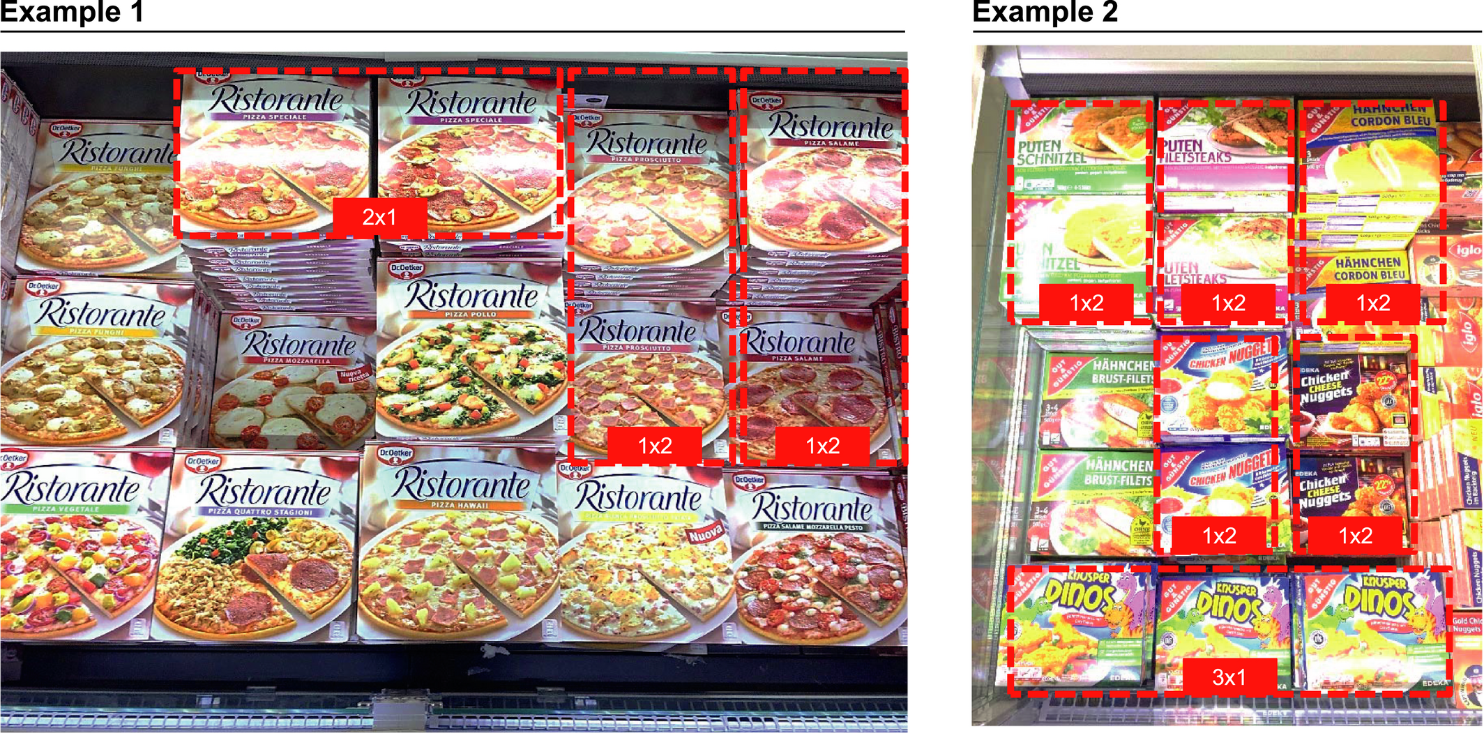
The rectangular requirement may result in “arrangement” and “prime number” defects if one‐dimensional solutions (e.g., 5 facings) are transferred to a two‐dimensional shelf setting (e.g., 2×2 facings). Arrangement defects occur if multiple rectangles (i.e., arrangements of different products) do not fit into one large rectangular arrangement (i.e., the shelf). Example 1 in Figure 4 shows this issue where not all facings of the optimal one‐dimensional solution can be placed on the shelf such as to maintain a rectangular shape. We use identically sized items to simplify the illustration. The total shelf space is 9 for the one‐ and two‐dimensional shelf. The optimal number of facings for the regular one‐dimensional shelf is A = 4 facings, B = 1 facings and C = 4 facings. On one‐dimensional shelves, an item with 4 facings is placed in one row (1×4), whereas on two‐dimensional shelves it can be placed in the form of 1×4, 4×1 or 2×2. Figure 4 shows that arranging both items A and C with 4 facings in a rectangular arrangement is not feasible as the total rectangular space is limited. The number of facings of item A or C therefore need to be reduced as only one item can have 4 facings. If, for example, item C now only has 3 facings, this may result in demand compensations by other items, and it may be preferable to list another item that compensates better the demand transfer between items.

Example 2 in Figure 4 presents the prime number defect. Due to the rectangular requirement, quantities with prime numbers (like 3,5,7,11,…) can only be arranged in a row (e.g., 1×3, 3×1, 1×5, 5×1, 1×7,…). However, if this row is larger than the total horizontal or vertical space, this is a non‐viable solution. The optimal number of facings of product A for a one‐dimensional shelf is 5 in Example 2. Since 5 is a prime number and is greater than the length or depth of the shelf, the item cannot be displayed in a rectangular manner. The defects can be expressed formally as follows. Consider S as the total (X×Y)‐dimensional space and

\bar{S}

its subset which represents the space currently unoccupied. Further, define the following set

R_{q_{i}} = (x \times y)

as the set of all possible rectangular arrangements of the one‐dimensional shelf quantity

q_{i}

of item i that needs to be assigned. The arrangement defect for an item i occurs if

\bar{S} \cap R_{q_{i}} = \emptyset

and the prime number defect for an item i occurs if

| R_{q_{i}} | = 0

Figure 4

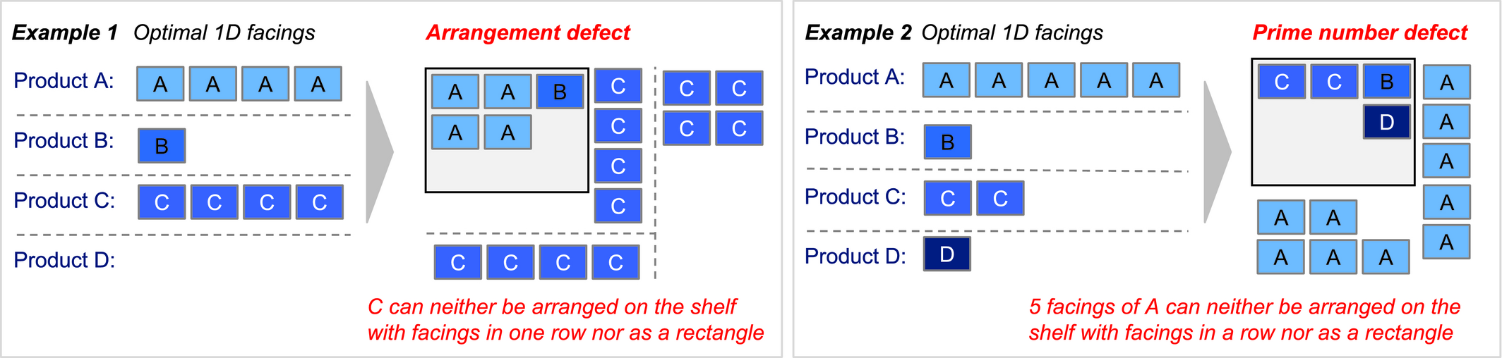
Characteristics of an Arrangement Defect (example 1) and a Prime Number Defect (example 2) [Color figure can be viewed at wileyonlinelibrary.com]

Summary. To create a planogram for two‐dimensional shelves, a shelf planner needs to make three simultaneous decisions for each category:

Item selection: This decision involves determining the assortment of a category.

Space assignment: This decision includes determining the number of horizontal facings, number of vertical facings, quantity per facing, and ultimately also the total shelf quantity for each product. The facings of one product can be arranged horizontally next to each other or vertically above one another. The total number of facings results from the multiplication of all vertical and horizontal facings.

Item arrangement: This determines which vertical and horizontal coordinates are assigned an item, that is, its exact location on the shelf. Furthermore, this also includes how different items are positioned next to each other (e.g., different types of bread next to each other). Finally, these all need to follow arrangement guidelines so that a rectangular shape is obtained and adjacent requirements are adhered to.

Two‐dimensional shelves are differentiated from regular shelves in terms of the options for space assignment and item arrangement. For regular shelves, it is sufficient to use one‐dimensional models to determine the horizontal number of facings. Two‐dimensional shelves require a definition of horizontal and vertical facings in a rectangular shape. These rectangular shapes however depend on the arrangement of other items. An integrated approach is therefore required that simultaneously solves the four subproblems item selection, shelf quantity, space assignment and item arrangement. Solutions obtained from familiar one‐dimensional models cannot be transferred directly to two‐dimensional settings for this purpose as one‐dimensional models lack the number of vertical facings and the item arrangement.

Related Demand Effects

All aforementioned decisions, namely item selection, space assignment and arrangement impact customer demand in three ways (see also Hübner and Schaal 2017a):

(1) Space‐elastic demand. The more facings an item are assigned, the higher its visibility on the shelf and the greater its demand. This demand effect is called space‐elastic demand. Various empirical studies include tests that quantify space‐elasticity effects (cf. Brown and Tucker 1961, Curhan 1972, Drèze et al. 1994, Eisend 2014, Frank and Massy 1970). Chandon et al. (2009) show that the variation of facings is the most significant in‐store factor, even stronger than pricing. Desmet and Renaudin (1998) reveal that space elasticities increase with the impulse buying rate. The magnitude of this demand increase depends on the item’s space‐elasticity factor, which indicates the percentage increase in demand of an item every time the number of facings goes up by a given amount. Using a meta‐analysis, Eisend (2014) identifies an average demand increase by a factor of 17%. Cross‐space elasticity measures responsiveness in the quantity demand of one item when the space allocated for another item changes. Eisend (2014) calculates an average cross‐space elasticity of −1.6%. Schaal and Hübner (2018) used numerical studies to show that the low empirical cross‐space elasticity values either do not have or have only very limited impact on optimal shelf arrangements. We therefore disregard cross‐space elasticities in the following. The demand impact of an item’s position can be neglected for two‐dimensional shelves. These positioning effects are relevant to regular shelves where e.g., eye‐ vs. knee‐level positions have a different demand impact. The same holds true for large categories where the shopper’s walking path and positions at the beginning, middle or end of an aisle matter. With two‐dimensional shelves, however, the basic idea is to allow the customer to oversee the total assortment of one (sub‐)category at one glance.

(2) Out‐of‐assortment and (3) Out‐of‐stock substitution demand. Customers can substitute for their choice if items are unavailable. For example, Gruen et al. (2002), Kök and Fisher (2007), Aastrup and Kotzab (2009) and Tan and Karabati (2013) show that between 45% and 84% of the demand can be substituted. Unavailability of items can result from two scenarios: either an item is delisted as a consequence of the assortment decision (out‐of‐assortment, OOA), or it is temporarily unavailable and currently not available on the shelf (out‐of‐stock, OOS). In both situations, customers may replace the unavailable items with other items which results in demand increases for the respective substitutes.

Substitution rates can be obtained by direct consumer surveys or by transactional data (e.g., Kök and Fisher 2007, Tan and Karabati 2013). A straightforward approach often applied to obtain substitution rates is to base them on market shares (Hübner and Kuhn 2012). This means that if an item has an overall demand share of 50%, the substitution rate from all products to this particular product is 50%. Finally, expert workshops can also be used to define substitution rates by selecting related items and rates.

Related Literature and Contribution

Current shelf planning literature focuses on regular shelf types (see also the reviews of Hübner and Kuhn 2012, Kök et al. 2015). We will first analyze this stream of literature and divide it into contributions that assume a given assortment and into contributions that integrate the assortment decision into shelf planning. This review is mainly used to gain insight into the different approaches for modeling demand and solution approaches. Secondly, we focus on particular applications to two‐dimensional shelf space problems. This review is used to define open research gaps and specify our contribution.

(1) Applications for regular shelves. Most shelf‐space optimization models assume deterministic demand and optimize the number of facings for items with space‐elastic demand to be assigned to limited shelf space. Respective approaches help retailers solve the trade‐off between more shelf space (and thus demand increases due to a higher number of facings) for certain items and less available space (and thus demand decreases due to a lower number of facings) for other items. One of the first models goes back to Hansen and Heinsbroek (1979) who formulate a shelf‐space model that accounts for space elasticity and solve it using a Lagrangian heuristic. Corstjens and Doyle (1981) develop a shelf‐space model that accounts for space and cross‐space elasticities which is solved via geometrical programming. Zufryden (1986) presents a dynamic programming approach with space‐elasticity effects. Lim et al. (2004) present a model that considers space and cross‐space elasticities for which they develop various extensions, e.g., for product groupings. A specialized heuristic and the combination of a local search and a metaheuristic approach are used to solve it. Hansen et al. (2010) develop a formulation with space and cross‐space elasticities for which they compare the performance of various heuristic and meta‐heuristic algorithms. The model also differentiates between horizontal and vertical shelf positions. Bianchi‐Aguiar et al. (2015) use a mixed‐integer programming approach to formulate a deterministic model that considers product‐grouping and display‐direction constraints and incorporates merchandising rules. Hübner and Schaal (2017b) formulate the first stochastic shelf‐space model that is solved with specialized heuristics. They account for space and cross‐space elasticity as well as vertical positioning effects. The model assumes a given assortment and does not incorporate substitution effects. In summary, the shelf‐space models mentioned assume a given assortment and optimize the number of facings. They do not take into account substitutions for unavailable items.

We further investigate contributions that integrate assortment decisions into their models in the following. Hübner (2011) develops a mixed‐integer model for shelf‐space planning that also takes assortment decisions into account. OOA situations are considered, but because the model assumes deterministic demand, OOS is ignored. Irion et al. (2012) use a piecewise linearization technique to solve a deterministic shelf‐space model that accounts for space and cross‐space elasticities. Although the model accounts for the assortment decision by setting facings to zero additional demand for OOA substitution is neglected. Hübner and Schaal (2017a) proposed the first integrated assortment and shelf‐space optimization model that accounts for stochastic demand, substitution, and space elasticity. To the best of our knowledge, they present the most comprehensive demand model. They showed that assortment and shelf planning are interdependent when shelf‐space is limited. A heuristic was developed to address large‐scale problems. The heuristic approach was modeled as an iterative MIP algorithm that uses recalculated precalculations for each step to circumvent the nonlinear problem. The integrated approach outperforms alternative approaches, e.g., a sequential planning approach that first picks assortments and then assigns shelf space.

(2) Applications for two‐dimensional shelves. Solutions obtained from one‐dimensional regular shelf settings, such as the above, cannot be transferred to two‐dimensional shelves due to arrangement and prime number defects. Only Geismar et al. (2015) have developed a model and solution approach for two‐dimensional shelves. They assume multiple shelves that are called cabinets. Each cabinet can have a distinct number of columns and rows. The capacity (or number of slots) of a shelf can be calculated by multiplying the columns and rows. Each product must have all of its units displayed within a single cabinet, and those units have to be displayed in a contiguous rectangle. All units need to have standardized unit sizes. To formulate the model in a more realistic and flexible manner, Geismar et al. (2015) did not divide cabinets into subsections to reduce the solution space or rather the complexity. Their formulation makes it possible to apply all the different dimensions of the product presentation within one cabinet according to the restrictions mentioned. In contrast to the majority of existing shelf‐space models, the objective is to maximize revenues rather than profit. Moreover, demand effects such as substitution or space elasticity were neglected. Apart from that, the demand is assumed to be deterministically known. However, the demand is affected by the effectiveness of a row. Each row can have a distinct effectiveness value. Due to the fact that the MIP approach did not find a solution within a two‐week time limit, they broke the problem into two subproblems. First, the products are assigned to the cabinets. Secondly, the units are arranged within the cabinets. The evaluation of observed data revealed an average revenue improvement of 3.7%.

Summary. Table 1 gives an overview of the main contributions. The demand models and solution approaches for regular one‐dimensional shelves have gradually been refined. Hübner and Schaal (2017a) present the most comprehensive model by integrating assortment and space allocation and taking relevant demand effects into account, that is, space‐elasticity, OOA and OOS substitutions. Previous literature suffers from one or more of the following drawbacks. First of all, only isolated optimization of either assortments or shelf‐space, ignoring the interdependence of both decisions. Secondly, limited consideration of relevant demand effects. Thirdly, applicability in practice is constrained by the limited assortment sizes that can be solved. None of the one‐dimensional shelf models integrate the vertical and horizontal arrangement of items. Geismar et al. (2015) presented the first extension for two‐dimensional problems and define the position of products. However, they apply a very restricted demand model and do not optimize assortments.

Table 1

Related Literature on Assortment and Shelf‐Space Optimization

We will base our extensions on the contributions of Geismar et al. (2015) and Hübner and Schaal (2017a). We contribute a new and more general approach by integrating assortment, space allocation and item arrangement decisions in a two‐dimensional shelf‐space setting. We further extend the demand model via space‐elastic demand and substitutions. This also includes the modeling of stochastic demand. Integrating demand volatility is relevant for retail settings (see e.g., Agrawal and Smith 1996 or Hübner et al. 2016), particularly for categories with perishable products (see e.g., Kök and Fisher 2007). This becomes even more important for two‐dimensional shelves as the majority of products kept on these shelves are perishable, e.g., fresh products like produce, products with limited sales periods like fashion and electronics. Finally, we relax the assumption of identical unit sizes as this does not hold true in most practical applications.

Development of the Decision Model

This section develops the Two‐Dimensional Stochastic Capacitated Assortment and Shelf‐space Problem (2DSCASP) in three steps: First, the decision model is formulated in section 3.1 which is then supplemented with the demand model in section 3.2. Finally, section 3.3 determines the arrangement and shelf space constraints. Table 2 shows the notation used.

Table 2

Notation

Indices and sets
i,j	Item indices
$N$	Total set of items
$N^{+}$ $(N^{-})$	Set of listed (delisted) items
R	Total set of rectangles
Parameters
$β_{i}$	Space elasticity of item i
$γ_{ji}^{OOA}$ $(γ_{ji}^{OOS})$	Share of demand of item j that gets substituted by item i in the event that item j is out‐of‐assortment (out‐of‐stock)
${\hat{δ}}_{i}$	Total expected demand of item i
$δ_{i}^{\min}$ $(f_{δ_{i}^{\min}})$	Minimum demand of item i (corresponding density function)
$δ_{i}^{sp}$ $(f_{δ_{i}^{sp}})$	Space‐elastic demand of item i (corresponding density function)
$δ_{i}^{OOA}$ $(δ_{i}^{OOS})$	Out‐of‐assortment (out‐of‐stock) demand of item i
$c_{i}$	Unit cost of item i
$d_{i}$ $(w_{i})$	Item depth (width) per unit of item i
$f_{i}^{*}$	Demand density function for i, generic form
$K_{i}$	Maximum number of facings of item i
$n_{ij}$	Binary parameter indicating whether item i has to be a neighbor of item j (=1) or not (=0)
N	Total number of items
$p_{i}$	Sales price for one unit of item i
$s_{i}$	Penalty cost for one unit of item i
$S^{width} (S^{depth})$	Total shelf width (depth) available
$v_{i}$	Salvage value for one unit of item i
Decision variables
$q_{i}^{x}$ $(q_{i}^{y})$	Integer number of facings of item i assigned in x‐dimension (y‐dimension)
$q_{i}^{t}$	Integer number of units of item i that are stacked behind one facing
$c o o r_{i}^{x}$ $(c o o r_{i}^{y})$	Integer location coordinate of item i in the x‐dimension (y‐dimension)
$l_{ij}$ $b_{ij}$ )	Binary variable denoting whether item i is arranged on the left of (below) item j (=1) or not (=0)
Auxiliary variables
$k_{i}$	Number of facings assigned to item i, with $k_{i} = q_{i}^{x} \cdot q_{i}^{y}$
$q_{i}$	Shelf quantity assigned to item i, with $q_{i} = q_{i}^{x} \cdot q_{i}^{y} \cdot q_{i}^{t}$
$z_{i}$	Binary variable indicating whether item i is selected in the assortment (=1) or not (=0)
$D_{i}$ $(W_{i})$	Space of item i occupied in a depth (width) dimension

Modeling the Decision Problem

The retailer must assign products of a particular category to a two‐dimensional shelf limited in size. That means considering a set of items

N

with

N = | N |

and optimizing the profit by simultaneously deciding

which products to list at all (item selection),

how much shelf space to allocate to the items listed (space assignment),

how the total item quantity is presented through horizontal and vertical facings in a rectangular shape, e.g., 4×1 or 2×2, and where the product is positioned, that is, x‐ and y‐coordinates of the shelf space (item arrangement).

We introduce various decision and auxiliary variables to express these decisions. We allow the shelf quantity

q_{i}

to be zero

(q_{i} = 0)

to account for delisting of items. The retailer must arrange the number of facings

k_{i}

, i = 1,2,…,N for each item N in a contiguous rectangular shape on the two‐dimensional shelf. The number of facings for the x‐dimension is expressed by the integer decision variable

q_{i}^{x}

and by

q_{i}^{y}

for the y‐dimension. The total number of facings

k_{i}

is therefore computed by

k_{i} = q_{i}^{x} \cdot q_{i}^{y}

. Since it is possible to stack each item, the entire shelf quantity

q_{i}

is computed by

q_{i} = k_{i} \cdot q_{i}^{t}

where

q_{i}^{t}

denotes the number of units of item i that are stacked behind each facing

k_{i}

, including the facing itself. We assume that there is no backroom storage which implies that all products listed have to fit onto the available shelf space. The retailer objective is to maximize total profit Π which is the sum of the item profits

π_{i}

of all items

i \in N

m a x i m i z e Π (\bar{q}) = \sum_{i \in N} π_{i} (q_{i})

(1)

The item profit

π_{i}

depends on the shelf quantity

q_{i}

for each item

i \in N

that is available for demand fulfillment. Items can be sold at the sales price

p_{i}

and are purchased for the unit costs

c_{i}

which incorporate all purchasing and processing costs (e.g., for replenishment). If the expected demand

D_{i}

for item i is greater than the shelf quantity

q_{i}

, the excess demand is lost and the retailer suffers the shortage costs

s_{i}

. Conversely, if items remain in stock at the end of the period, they need to be disposed of at a salvage value

v_{i}

and the retailer incurs a loss, because

v_{i} < c_{i}

The profit for each item is calculated as shown in Equation 2 and consists of the following elements: The first term represents the overall purchasing costs, the second and fourth term calculate the expected revenues, the third term represents the expected revenues from leftover items sold for the salvage value, and the fifth term calculates the penalty costs in the event of stockouts. This generic form of the item profit

π_{i}

corresponds to the profit calculation in newsvendor problems and can therefore also be found in many other assortment related decision models (e.g., Hübner et al. 2016, Kök and Fisher 2007, Smith and Agrawal 2000). The difference always stems from the demand that is taken into account which is represented by the density function

f_{i}^{*}

. This probability density function

f_{i}^{*}

in Equation 2 accounts for the relevant total demand distribution which must be quantified in accordance with the assumed customer behavior. In our case, the density function must take into account OOA and OOS substitution as well as the space‐elastic demand. We investigate the related demand function in more detail below.

\begin{matrix} π_{i} (q_{i} |_{q_{i} = q_{i}^{x} \cdot q_{i}^{y} \cdot q_{i}^{t}}) = & - c_{i} \cdot q_{i} + p_{i} \cdot \int_{0}^{q_{i}} y f_{i}^{*} d y \\ + v_{i} \cdot \int_{0}^{q_{i}} (q_{i} - y) f_{i}^{*} d y + p_{i} \cdot \int_{q_{i}}^{\infty} q_{i} f_{i}^{*} d y \\ - s_{i} \cdot \int_{q_{i}}^{\infty} (y - q_{i}) f_{i}^{*} d y \end{matrix}

(2)

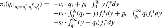
The model does not force the user to completely fill the available shelf space. It is permitted to leave free spaces due to penalty costs for oversupply. In constellations with large shelves, low demand and high oversupply costs, for example, there could be situations where the full space is not used. However, this is assumed to be rather a hypothetical situation due to general space constraints in retail stores.

Modeling the Demand Function

The probability density function

f_{i}^{*}

of the standard newsvendor formulation needs to be enriched in order to consider different demand effects. Because items can be delisted, we divide the set of all items

N

into listed items

(N^{+})

and delisted items

(N^{-})

in the following, such that

N^{+}, N^{-} \subseteq N

N^{+} \cup N^{-} = N

and

N^{+} \cap N^{-} = ⊘

. The total expected demand

{\hat{δ}}_{i}

of an item i consists of three elements (see Equation 3). The first is space‐elastic demand

δ_{i}^{sp}

which is driven by the number of facings. Next is the OOA demand

δ_{i}^{OOA}

which depends on whether the items j, for which i is a substitute (j≠i) are listed

(q_{j} > 0)

or not

(q_{j} = 0)

. The third is OOS demand

δ_{i}^{OOS}

which depends on the available shelf quantity q of the other items j (j≠i). We elaborate on the three demand components below.

{\hat{δ}}_{i} = δ_{i}^{sp} + δ_{i}^{OOA} + δ_{i}^{OOS} i \in N

(3)

Space‐elastic demand. Customer demand for an item grows with the number of facings assigned for this item. The magnitude of the demand increase depends on the space elasticity

β_{i}

, the number of facings

k_{i}

and the minimum demand

δ_{i}^{\min}

. The space‐elastic demand is denoted by

δ_{i}^{sp} (k_{i})

and calculated corresponding to Equation 4. The corresponding density is denoted by

f_{δ_{i}^{sp}}

δ_{i}^{sp} (k_{i} |_{k_{i} = q_{i}^{x} \cdot q_{i}^{y}}) = δ_{i}^{\min} \cdot k_{i}^{β_{i}} i \in N

(4)

The space‐elastic demand grows with a diminishing rate with

k_{i}^{β_{i}}

for k > 1. The minimum demand

δ_{i}^{\min}

is equal to the demand of an item if it were represented with one facing (

k_{i} = 1

), that is,

δ_{i}^{\min} = δ_{i}^{sp} (k_{i} = 1)

(cf. Bianchi‐Aguiar et al. 2015, Corstjens and Doyle 1981, Hansen and Heinsbroek 1979, Hansen et al. 2010, Irion et al. 2012, Urban 1998, or Hübner and Schaal 2017a).

The space‐elastic demand for an item i with

k_{i} = 0

mathematically results in no demand as

δ_{i}^{sp} (k_{i} = 0) = δ_{i}^{\min} \cdot 0^{β_{i}} = 0

. This does not hold true since some customers would still want to buy the item even if it was not shown on the shelf anymore. To factor in this effect, we assume the identical minimum demand for a product with no facings as if it had exactly one facing. In other words, the demand with one facing is described as the minimum demand even if a product is delisted. In cases of

k_{i} = 0

, this means we assign space‐elastic demand by applying

δ_{i}^{sp} (k_{i} = 0) = δ_{i}^{\min}

. The corresponding density function for the minimum demand is denoted by

f_{δ_{i}^{\min}}

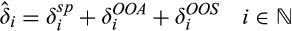
Out‐of‐assortment demand. OOA demand for a listed item i (

i \in N^{+}

) occurs if another item j is delisted (

j \in N^{-}

) and customers substitute this item j with item i. We assume that if item j is delisted, customers substitute a certain share

γ_{ji}^{OOA}

of the minimum demand

δ_{j}^{\min}

of item j with item i, because some customers will still want to buy item j, even if it is not listed. The maximum quantity that can be substituted of item j cannot be higher than the minimum demand of the item j. This is first due to the aforementioned assumption that the space‐elastic demand in the event of k = 0 corresponds to the minimum demand, and secondly because we follow the usual assumption that substitution takes place over one round only (cf. e.g., Gaur and Honhon 2006, Hübner et al. 2016, Kök and Fisher 2007, Ryzin and Mahajan 1999, Smith and Agrawal 2000). This simplification is common across most assortment literature (cf. Kök et al. 2015). If consumers want to substitute their first choice by a product that is not available, the demand is lost as a result. There is no attempt to model individual consumer decisions. Instead, an exogenous model is applied that is capable of capturing aggregated consumer demand. The resulting model is cruder than some other substitution models but has the advantage of being much easier to analyze and requiring less data. That also means that demand is uniform across time. To summarize, this implies that demand is lost if a substitute is not available either. Therefore, if an OOA item is a substitute for another non‐available item, the additional substitution demand for the OOA item would only occur if it was available. The OOA demand of an item i is calculated as follows:

δ_{i}^{OOA} = \sum_{j \in N^{-}, j \neq i} δ_{j}^{\min} \cdot γ_{ji}^{OOA} i \in N

(5)

The density function for OOA demand for item i is calculated by Equation 6. Since we assume that the distributions of the minimum demand of two items i and j, i≠j, are independent, the convolution – represented by the operator

⊛

– can be used to calculate the distribution of the sum of the demand of the two items (cf. Hübner et al. 2016). Equation 6 convolutes the (minimum) demand distribution functions of all delisted items and therefore accounts for the fact that the OOA substitution demand for item i depends on all delisted items

j \in N^{-}

. To simplify, we have omitted the

γ_{ji}^{OOA}

parameters in the equation.

⊛_{j \in N^{-}} f_{δ_{j}} = \int \dots \int_{R_{0}^{+, n}, j \in N^{-}} f_{δ_{j}^{\min}} d τ \dots d υ

(6)

Out‐of‐stock demand. OOS demand for a listed item i

i \in N^{+}

occurs if another listed item j

j \in N^{+}

is temporarily out‐of‐stock, that is, if demand for item j exceeds the available shelf quantity of item j. In this case, we assume that customers substitute a certain share of the shortage quantity of item j with item i. The shortage quantity of item j is calculated via

δ_{j} - q_{j} | δ_{j} > q_{j}

and the substitution share denoted by

γ_{ji}^{OOS}

. Equation 7 shows the OOS demand calculation (also see e.g., Hübner et al. 2016, Kök and Fisher 2007, Rajaram and Tang 2001):

δ_{i}^{OOS} = \sum_{j \in N^{+}, j \neq i} [(δ_{j} - q_{j}) | δ_{j} > q_{j}] \cdot γ_{ji}^{OOS} i \in N

(7)

Equation 8 depicts the density function for OOS demand for item i. As above, we use the convolution to account for the fact that OOS demand for an item i depends on the expected shortage of all temporarily unavailable items other than item i.

⊛_{j \in N^{+}} f_{δ_{j}} = \int \dots \int_{q_{j}, j \in N^{+}}^{\infty} f_{δ_{j}} d τ \dots d υ

(8)

Modeling the Arrangement and Space Constraints

Before we specify the constraints of our problem, we give a broader context on the modeling of the arrangement constraints which also impacts the solution approach later on.

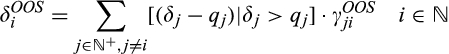
General modeling approach. Our problem belongs to the class of Two‐Dimensional Knapsack Problems. These problems deal with the selection and arrangement of a set of rectangles r ∈ R to a capacitated two‐dimensional rectangular container S with a certain width

S^{width}

and depth

S^{depth}

. In our case, the rectangle r represents not the item i itself but its facings

k_{i}

and the corresponding width dimension

W_{i}

, depth dimension

d_{i}

, as well as its profit value

π_{i}

. Selected rectangles need to be orthogonally placed in the container and are not allowed to overlap the container limits (Bortfeldt and Winter 2009). Different constraints are applicable to this problem. First, with regard to the number of reproductions of each rectangle, our problem belongs to the Single‐Constrained Knapsack Problems (c.f. Beasley 2004, Bortfeldt and Winter 2009). In our case, each rectangle represents a certain facing number and its arrangement of a certain item that needs to be allocated to a single container. We need to apply an upper limit that restricts the maximum size of a rectangle but the item selection included ensures that no lower bound is set (as for doubly constrained Knapsack problems). The second constraint type is the orientation constraint that determines whether a rectangle can be rotated by 90 degrees to fit onto the container or not (c.f. Lodi et al. 1999). In our case, the dimension of a rectangle is dictated exogenously because the rotation of the rectangles is not allowed (e.g., because product labels need to be legible and the display is defined). A final differentiation is the guillotine cutting constraint that can be applied to divide the total solution space into parts. A container is divided into sections by using guillotine cuts. Guillotine cuts can be made horizontally or vertically and from one side to the opposite (“edge‐to‐edge”) of the container, whereas one item can only belong to one container (=subsection). Each resulting subsection is considered separately and may be cut again. This procedure reduces the solution space as less combinatorial options are possible. Figure 5 depicts a guillotine and non‐guillotine approach applied to a two‐dimensional shelf. Our application does not allow guillotine cuts as this would reduce the degrees of freedom for how facing and arrangement options can be chosen within the container. The variable dimensions of the rectangle would also not allow meaningful cuts. According to the typology of Wäscher et al. (2007), the 2DSCASP is a Single Large Object Placement Problem that is transformed by the item consolidation to a Single Knapsack Problem.

Figure 5

Guillotine Cutting Patterns [Color figure can be viewed at wileyonlinelibrary.com]

Specification of arrangement and space constraints for 2DSCASP. We use the relative arrangement formulation of Pisinger and Sigurd (2007) as it meets the requirements of our application summarized above. This ensures proper arrangement of the selected items with their corresponding dimensions. We introduce the auxiliary variable

z_{i}

for the assortment decision to simplify the notation with

z_{i} = \{\begin{matrix} 1 for q_{i} \geq 1 \\ 0 else \end{matrix} \forall i \in N

. The two boolean decision variables

l_{ij}

and

b_{ij} (i \neq j) \in {0, 1}

∀i,j ∈ N determine whether or not item i is arranged to the left of item j

l_{ij}

and/or below

b_{ij}

within the shelf space. Equation 9 ensures that all selected items have a position relative (left or/and below) to one another. The binary parameter

n_{ij}

indicates whether or not item i has to be a neighbor of item j. This allows the definition of joint positioning for related products within a category (e.g., rye bread belongs to the category bread). Equations 10–12 define required neighborhood constraints accordingly. Restriction (10) prevents diagonal neighborhoods, whereas restrictions (11) and (12) ensure that the borders of the item quantities

q_{i}

and

q_{j}

have adjacent edges for a certain stretch.

The two‐dimensional shelf‐space limits are represented by

S^{width}

for the width (x‐dimension) and

S^{depth}

for the depth (y‐dimension). Due to the fact that the dimensions of one item only represent the space occupied by the rectangle (rectangularly shaped quantity of one item) in the special case

q_{i} = 1

, we introduce the auxiliary variables

W_{i}

and

D_{i}

in restriction (13) and (14) that represent the space occupied. The parameters for width

w_{i}

and depth

d_{i}

represent the space occupied by all units of the item i. The decision variables for the coordinates that indicate the lower left position of the item’s display are denoted by

c o o r_{i}^{x}

for the x‐ and

c o o r_{i}^{y}

for the y‐coordinate. Equations 15 and 16 ensure that the items N do not overlap each other within the shelf space. Restrictions (17) and (18) guarantee that no item i crosses the border of the shelf space. In equation 19, a maximum facing limit of item i is set. This gives retailers the opportunity to ensure a variety of different products on their shelves by setting the parameter

K_{i}

. Equations 20 define the domain of the variables.

l_{ij} + l_{ji} + b_{ij} + b_{ji} \geq z_{i} + z_{j} - 1 \forall i, j (i \neq j) \in N

(9)

l_{ij} + l_{ji} + b_{ij} + b_{ji} \leq 3 - n_{ij} \cdot z_{i} - n_{ij} \cdot z_{j} \forall i, j (i \neq j) \in N

(10)

c o o r_{i}^{x} + W_{i} - c o o r_{j}^{x} \leq S^{width} (1 - l_{ij} \cdot n_{ij}) \forall i, j (i \neq j) \in N

(11)

c o o r_{i}^{y} + D_{i} - c o o r_{j}^{y} \leq S^{depth} (1 - b_{ij} \cdot n_{ij}) \forall i, j (i \neq j) \in N

(12)

W_{i} = w_{i} \cdot q_{i}^{x} \forall i \in N

(13)

D_{i} = d_{i} \cdot q_{i}^{y} \forall i \in N

(14)

c o o r_{i}^{x} + W_{i} \leq c o o r_{j}^{x} + S^{width} (1 - l_{ij}) \forall i, j (i \neq j) \in N

(15)

c o o r_{i}^{y} + D_{i} \leq c o o r_{j}^{y} + S^{depth} (1 - b_{ij}) \forall i, j (i \neq j) \in N

(16)

0 \leq c o o r_{i}^{x} \leq S^{width} - W_{i} \forall i \in N

(17)

0 \leq c o o r_{i}^{y} \leq S^{depth} - D_{i} \forall i \in N

(18)

K_{i} \geq k_{i} \forall i \in N

(19)

\begin{matrix} l_{ij}, b_{ij}, z_{i} \in {0, 1}; \\ q_{i}^{x}, q_{i}^{y}, q_{i}^{t}, q_{i}, k_{i}, c o o r_{i}^{x}, c o o r_{i}^{y} \in Z_{0}^{+} \forall i, j (i \neq j) \in N \end{matrix}

(20)

Heuristic Approach

The 2DSCTSP is compounded by the NP‐hard two‐dimensional Knapsack Problem (see Beasley 2004, Kellerer et al. 2004, Pisinger 2005, Pisinger and Sigurd 2007) and the NP‐hard assignment problem (see Hübner et al. 2016, Kök and Fisher 2007). The combinatorial complexity of the latter increases very rapidly with the number of items being considered, N, and the shelf‐space size S. The total number of possible allocations (Y) to a one‐dimensional container can be calculated as expressed by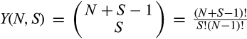

Y (N, S) = (\begin{matrix} N + S - 1 \\ S \end{matrix}) = \frac{(N + S - 1)!}{S! (N - 1)!}

. For example, an instance of N = 5 and S = 10 results in 1,001 and an instance of N = 50 and S = 100 in

6.7 \cdot 10^{39}

possible solutions. The two‐dimensional problem is even more complex. Here, one obtains up to

N^{S}

combinations without any arrangement rules (rectangle, coherent). In the first example, the number of combinations increases to 9,765,625 and in the second example to

7.9 \cdot 10^{169}

combinations. Furthermore, the demand characteristics result in a profit function

π_{i}

for each item i (Equation 2), which is nonlinear with respect to the decision variables. A metaheuristic approach is therefore developed – a genetic algorithm (GA) suitable for solving real world problems sufficiently and efficiently. We propose a GA paired with a one‐dimensional start solution and a bottom‐left fill (BLF) heuristic.

Structure and notation. We will use the general algorithmic‐related terms “container” and “rectangle.” A set of small rectangular pieces has to be allocated to a larger rectangle, known as a container. In our application, the container is equal to a shelf and a rectangle represents certain facing and arrangement options of a certain item. The algorithm is developed with object‐oriented programming standards to avoid a complex de‐/encoding of the solution of each individual object. Instead of complex encryption to represent the different rectangles with their corresponding attributes, the references of the objects are taken into account to execute genetic operations. This ensures that no information is lost while performing the operations and all attributes are accessible at any time. The decoding is implemented as an object function that invokes the operation that arranges the rectangles onto the container and calculates the fitness of the individual. Extensive en‐/decoding to or of a binary, a permutation or a value notation are not necessary. We refer to Keijzer et al. (2002), Krishnamoorthy et al. (2002) and Zhang and Wong (2015) for similar implementations of object‐oriented evolutionary algorithms. The necessary components for the implementation are detailed in the Appendix with the help of Unified Modeling Language (UML).

Pseudo Code. Algorithm 1 summarizes the sequential, procedural program flow. This is a specialized heuristic tailored to our problem and based on a GA. We apply different settings for the various steps of the algorithm as summarized in Table 3.

Algorithm 1 Genetic algorithm for 2DSCTSP
Require: N, $S^{width}$ , $S^{depth}$ , termination criterion
Ensure: fittest individual over all generations
1: possibleArrangements ← generateArrangements(N, $S^{width}$ , $S^{depth}$
2: population ← generateStartPopulation(possibleArrangements)
3: allocateProducts(population)
4: formerFittestIndividual ← calculateFitness(population)
5: While (termination criterion False) do
6: population ← selectAndDuplicateFittest(population)
7: population ← crossoverOperation(population)
8: population ← mutationOperation(population)
9: allocateProducts(population)
10: currentFittestIndividual ← calculateFitness(population)
11 population ← elitismOperation(currentFittestIndividual, formerFittestIndividual)
12: formerFittestIndividual ← saveFittestIndividual(formerFittestIndividual, currentFittestIndividual)
13: end While
14: printFittest(formerFittestIndividual)

Table 3

Configuration Settings of the Genetic Algorithm

Step and method	Possible settings
Step 2: Start solution	Random, Adapted one‐dimensional solution
Step 3: Rectangle allocations	Bottom‐left fill heuristic
Step 5: Termination criterion	Runtime, Number of populations, Solution quality
Step 6: Selection	Wheel, Tournament, Rank
Step 7: Crossover	Fixed, Random
Step 8: Mutation	Probability rate and variance configurable
Step 11: Elitism	Injection rate of the previous fittest solution

The algorithm starts with input of the set of items N, shelf dimensions

S^{width}

and

S^{depth}

, and the termination criterion. The objective is to find the fittest individual across all generations, which contains the container with the most profitable rectangles.

Step 1 generates the set of possible rectangles for each item, i ∈ N. It takes into account the shelf dimensions

S^{width}

and

S^{depth}

. The number of maximum facings

K_{i}

(i ∈ N) is denoted by the shelf dimensions. The possible arrangement options for each item are generated as a result of the maximum quantity in each visible shelf dimension

S^{width} / w_{i} \geq q_{i}^{x}

S^{depth} / d_{i} \geq q_{i}^{y}

and exclusion of arrangement options that result in prime number defects.

Following Step 2 generates a start population. We implemented two different options. In the simple case, a random start solution (RSS) is applied. In the advanced version, an adapted one‐dimensional start solution (ASS) is generated using the model and solution approach of Hübner and Schaal (2017b). They develop an iterative heuristic that solves a MIP for the assortment and space allocation problem in the first step and, in the subsequent step, updates the demand calculation according to the shelf configuration of the first step. This procedure is repeated until a solution‐quality‐related termination criterion is met. We extend this approach by using a constraint in the MIP to directly eliminate the prime number facings that exceed one

S^{width}

S^{depth}

. The arrangement issue that items cannot be allocated to the shelf because of their particular dimensions cannot be included in Hübner and Schaal (2017b). The computed one‐dimensional quantities are subsequently transformed into two‐dimensional feasible arrangements.

Step 3 allocates the rectangles to containers. So far, the algorithm is composed of a population of individuals where each individual consists of a single container that contains one or multiple rectangles and where each rectangle has an item reference. We use the BL‐F pack heuristic to fill up the containers. Hopper and Turton (2001) identified the BL‐F as an efficient approach for the two‐dimensional packing problem. The BL‐F is a modified version of the bottom‐left (BL) pack heuristics. The BL algorithm starts with placing each rectangle in the top right corner of the container. From there, the rectangle slides as far as possible (without crossing another item) to the bottom and then as far as possible to the left of the container. This movement process is repeated until the rectangle can no longer be moved, that is, the rectangle collides with another rectangle or the frame of the container. This makes full use of the rectangle. The disadvantage of the BL algorithm is the empty space within the container. In contrast to this, the BL‐F algorithm seeks the lowest left position in the container that the rectangle can fit into. This approach makes it possible to occupy what were previously empty spaces but also leads to a higher runtime. Furthermore, Hopper and Turton (2001) show computational benefits if the rectangles are sorted and filled by size

W_{i} \cdot D_{i}

in descending order. Note that the algorithm is not forced to completely fill up the shelf space. It may be better to leave free spaces within the shelf due to penalty costs for oversupply in the objective function.

After this, rectangles are allocated and the fitness of each individual is evaluated in Step 4. The algorithm is terminated based on maximum runtime, number of populations or solution quality improvements. If the termination criterion in Step 5 is met, the fittest individual is displayed. Otherwise, the loop of Steps 6 to 11 is executed until the termination criterion is met.

Steps 6 to 8 describe the GA operator’s selection, crossover, and mutation. The selection operation in Step 6 intensifies the average fitness of a population through duplication of the fittest and disposal of the weakest individuals. We use different approaches. In wheel selection (WS), the selection probability of an individual is calculated by dividing the fitness of a selected individual by the total cumulative fitness of all individuals. This approach ensures that stronger individuals are more likely to be included in the adapted population than weaker ones. Tournament selection (TS) is based on the comparison of two randomly picked individuals of a population. The individual with the higher fitness score is selected for the adjusted population. All chosen or not chosen individuals remain in the basic population and can be selected again. Rank selection (RS) reevaluates the fitness of each individual depending on the fitness ranking. The technique takes the rank of the fitness value and not the nominal value into account. A common approach is to rate the worst as fitness 1, the second worst as fitness 2, and so on. The best is rated as N, where N equals the number of individuals considered.

The crossover operation in Step 7 is a method for interbreeding the individuals of the selected population to form a new offspring population. Crossover is performed with a specified probability rate. The crossover operation can be executed with a fixed number or randomly generated amount of crossover points. The points are most evenly divided depending on the quantity of items, that is, to build equal sized crossover parts the length of the individual is divided by the amount of crossover points, whereby the last part contains the size of the modulo value. All items between the crossover points alternately remain part of the individuals or swap between the individuals. In the mutation operation in Step 8, small segments of the individuals of the new offspring are randomly modified. The purpose of this is to preserve diversity across generations. The mutation probability rate and the variance of the modification can be chosen. During the execution, the new quantity of the item is also randomly transferred to feasible two‐dimensional spaces.

In Steps 9 to 12, all rectangles within each individual are allocated and evaluated. Crossover and mutation operations modify individuals so much that there is a high probability of losing the fittest individual across the following generations. Hence, an elitism method is applied to preserve the fittest individual across the next generations. The overall fittest individual is saved and injected into a population if the fittest individual of this population is not at least as fit as the fittest overall. The fittest individual of this generation is compared with the individual that is fittest overall to determine the new individual that is fittest overall. Then the algorithm returns to Step 5.

Numerical Results

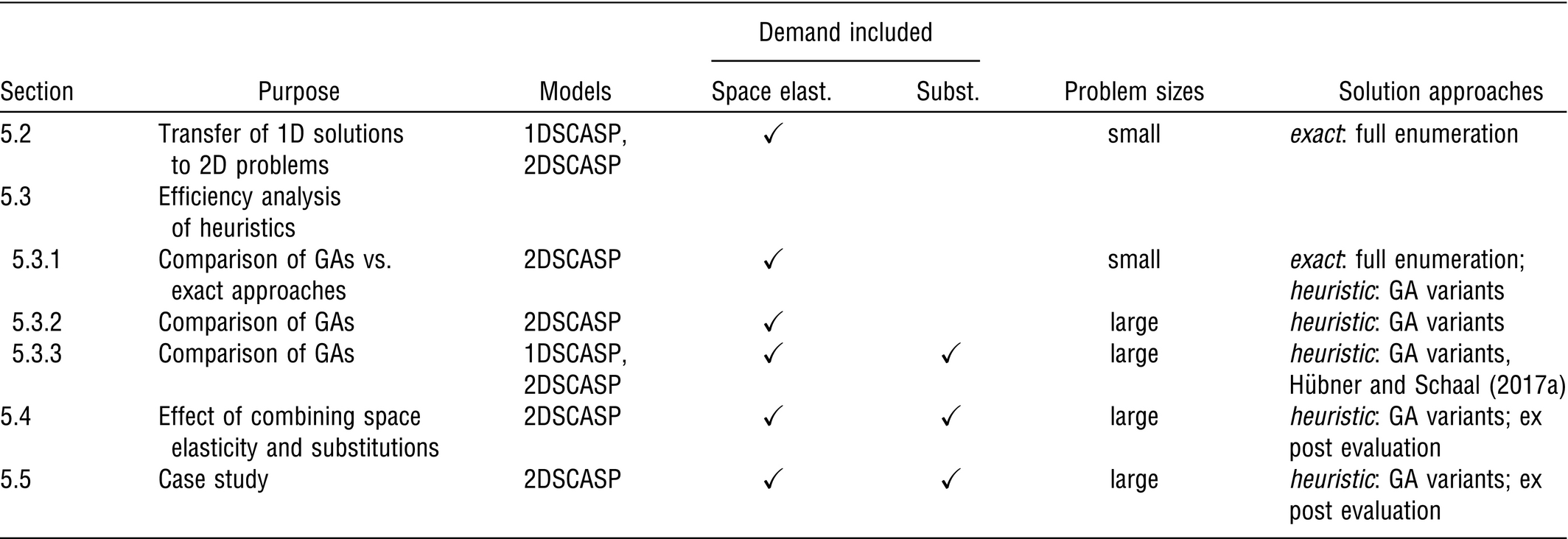
In this section, we first describe the test setting before then conducting various numerical analyses with simulated data and data from a case study and different variants of the model. We gradually increase the complexity to demonstrate the efficiency of the models and solution approaches step by step. Section 5.2 investigates the error range if the solutions of a one‐dimensional model (1DSCASP) are transferred to a two‐dimensional problem (2DSCASP). The heuristic approaches are analyzed and compared in terms of runtime and solution quality in section 5.3. Section 5.4 assesses the impact of demand effects and correctly accounts for stochastic demand, space elasticity, and substitution on profit as well as facing changes. Finally, we apply our model to a case study in section 5.5. Table 4 gives an overview.

Table 4

Overview of Numerical Tests

Data Generation and Test Setting

To generalize our analysis, all input parameters are randomly generated within sections 5.2–5.4. We generated parameter values within reasonable ranges derived from literature or from the cooperation with a retailer. There are either sources from empirical studies (e.g., Campo et al. 2004, Gruen et al. 2002 or Aastrup and Kotzab 2009 for the range of substitution rates; Desmet and Renaudin 1998, Drèze et al. 1994 or Eisend 2014 for space‐elasticity effects) or from other comparable modeling approaches (e.g., Hübner et al. 2016, Kök and Fisher 2007 for the ranges of profits and over‐/undersupply costs). In generating our data sets, we thus used conventional practice and followed the suggestions of previous literature. We made the data available at GitHub (https://github.com/fabSchaefer/2DSCTSP). These are equally distributed and satisfy the following rules. Each item i ∈ N has a positive profit

r_{i} > c_{i}

, a positive salvage value

v_{i}

and positive shortage costs

s_{i}

. The ratio pattern between the parameters is defined as

r_{i} \geq c_{i} \geq v_{i} \geq s_{i}

with r ∈ [20;25], c ∈ [4;9], v ∈ [4;9] and s ∈ [1;3]. Hübner et al. (2016) reveal that continuous demand distributions serve as good approximations of discrete demand distributions. It is assumed that demand is normally distributed with an average minimum demand of

μ_{i} \in [7; 25]

and a corresponding coefficient of variation

C V_{i} \in [1 %; 40 %]

. Modeling demand volatility with

C V_{i}

ensures that negative demand cannot occur. The space elasticity β is assumed to vary between 0 ≤ β ≤ 0.40 (cf. Eisend 2014). According to Campo et al. (2004) the OOA substitution rates are suitable for providing approximations for OOS substitution rates. Without compromising the general applicability of our model, we assume that the substitution rates for OOA and OOS are the same, that is,

γ_{ji}^{OOA} = γ_{ji}^{OOS}

, ∀i,j ; j≠i. To simplify, we denote the probability that an unavailable item i gets substituted by the aggregated substitution rate

λ_{i}

and assume that this rate is split equally among all other items such that

γ_{ji}^{OOA} = γ_{ji}^{OOS} = \frac{λ_{i}}{N - 1}

, ∀i,j ; j≠i. To focus on the core demand effects, we assume that all items have a uniform size with an identical depth and width of

d_{i} = w_{i} = 1

and a shelf stock per facing of

q_{i}^{t} = 1

. If not stated otherwise, we considered 100 randomly generated instances for each problem setting. For all instances of a problem setting the assortment size N and shelf size

S^{width} \times S^{depth}

are assumed to be identical. All numerical tests were conducted on a Windows Server 2012 R2 64‐bit with two Intel Core E5‐2620 processors and 64‐GB memory. The tests are implemented in VB.net (Visual Studio 2019) and GAMS 27.2.

Transfer of One‐Dimensional Solutions to Two‐Dimensional Problems

The one‐dimensional solution is easier to obtain, but it may not be a feasible solution due to arrangement and prime number defects (also see section 2). This analysis serves to assess the error impact of transferring solutions obtained by models that are based on one‐dimensional shelf space to settings with two‐dimensional shelf space. The best case would show that one‐dimensional solutions are a good approximation for the two‐dimensional problems. We solve the following three models exactly: 1DSCSP includes prime numbers, 1DSCSP

_{ex - prim}

excludes prime numbers and 2DSCSP. Six test problem settings are defined with a varying total number of items (N), quadratic shelf sizes with

S^{width} = S^{depth}

and an upper limit on the facings

K_{i} = S^{width} \times S^{depth}

. The randomly generated demand of each item is set to [1;6] for sets 1 to 4 and [1;9] for sets 5 to 6. These problem sizes ensure computationally tractable runtimes. For each problem 100 instances are randomly generated by using the data ranges provided above.

Frequency of defects. Table 5 reveals the occurrence of defects. The arrangement and prime number defect of the one‐dimensional solution appear in all settings. Arrangement defects can be found in 14% and prime number defects in 32% of the cases. In some cases both defects exist. Consequently, one or both defects occur in 41% of cases.

Table 5

Analysis of Arrangement Defects of 1D Solutions, Average of 100 Instances

Number of items N	4	5	6	7	6	6	Total
Total shelf space $S^{width} \times S^{depth}$	3×3	3×3	3×3	3×3	4×4	5×5	Total
Arrangement defect [%]	15	9	14	2	18	24	14
Prime number defect [%]	27	29	23	26	56	33	32
Total cases with defect/s [%]	37	32	31	28	66	51	41

Profit impact of defects. Table 6 summarizes the profit impact due to the required arrangements on a two‐dimensional shelf. It compares the exact solutions of the 2DSCSP with the 1DSCSP. The latter do not consider the rectangular arrangement and prime number requirements, whereby 41% of 1DSCSP solutions are non‐viable solutions for the 2DSCSP. These additional requirements in the two‐dimensional problem lower the profit by 0.8% on average. Hence, this expresses the total profit impact caused by the rectangular arrangement and prime number constraint. In other words, theoretically the feasible solution yields 0.8% lower profit compared to the non‐viable solution without prime number and arrangement constraints.

Table 6

Profit Comparison of 2DSCSP vs. 1DSCSP, 100 Instances

Number of items N	4	5	6	7	6	6	Total
Total shelf space $S^{width} \times S^{depth}$	3×3	3×3	3×3	3×3	4×4	5×5	Total
Average profit¹	0.991	0.989	0.992	0.994	0.992	0.997	0.992

¹Calculation: 2DSCASP profit / 1DSCASP profit

Arrangement and prime number defect. To quantify the individual profit impact for each type of defect, we compare the 1DSCSP and the 1DSCSP

_{ex prime}

where prime numbers are excluded. The results in Table 7 depict that the prime number defect leads on average to a 0.5% lower profit. Hence, imposing the arrangement constraints results in 0.3% lower profits.

Table 7

Profit Comparison of Exact Solutions: 1DSCSP

_{ex - prime}

vs. 1DSCSP, 100 Instances

Number of items N	4	5	6	7	6	6	Total
Total shelf space $S^{width} \times S^{depth}$	3×3	3×3	3×3	3×3	4×4	5×5	Total
Average profit¹	0.995	0.991	0.996	0.995	0.995	0.999	0.995

¹Calculation: 1DSCSP

_{ex - prime}

profit / 1DSCASP profit

Summary. The one‐dimensional solution is easier to obtain, however, it is not a feasible solution due to arrangement and prime number defects. These requirements impact optimal allocation. The optimal item quantities of the two‐dimensional problem differ from those of the one‐dimensional problem. Due to the additional constraints in the 2DSCSP, the total profit will always be equal or below the 1DSCSP. The corresponding one‐dimensional solution approaches are not readily appropriate methods for solving two‐dimensional problems. It has to be considered that in cases where the one‐dimensional solution does not fit onto the two‐dimensional shelf space, quantities of items need to be adjusted. It is not obvious which item quantities have to be increased or decreased to achieve the best feasible solution (e.g., via simple rounding or greedy heuristics). The decision process becomes even harder when substitution effects in the model are considered due to the demand interdependencies between the items. The consequence of this is that the loss in solution quality would be significantly higher if using the one‐dimensional model.

Efficiency Analysis of Heuristics

Comparison of Heuristics with Space Elasticity vs. Exact Approaches

This section examines the efficiency of the heuristic developed. To validate the GA it is compared to a full enumeration (FE) applied to smaller problem sizes. The GA is executed as described in section 4 with a RSS and the selection methods WS, TS, and RS. The random crossover operation and the elitism operation are applied. Mutation operations are not reasonable and can be neglected due to the small size of problem instances. Pretests have shown that a termination criterion of 100 seconds is more than sufficient to return the best solution.

Runtime. Table 8 summarizes the computation time. For the FE, it shows that the median runtime increases between four to ten times if the set is extended by only one additional item. A similar magnitude is recognizable when the space is extended gradually. For the different implementations of the GAs, the runtime is significantly lower and the increases for extended problem sizes are much lower. Furthermore, the runtimes of the WS and TS are below 4 seconds on average in all instances. The smallest median execution time across all 600 problem instances was achieved via the TS, and is over 120 times faster than the FE.

Table 8

Median Runtime of Different Approaches, in seconds, 100 Instances

Number of items N		4	5	6	7	6	6	Total
Total shelf space $S^{width} \times S^{depth}$		3×3	3×3	3×3	3×3	4×4	5×5
FE	Median	0.728	2.530	22.593	135.332	72.136	134.920	19.988
GA WS	Median	0.171	0.327	0.547	1.028	2.106	3.117	0.788
GA TS	Median	0.036	0.087	0.130	0.220	0.376	0.710	0.164
GA RS	Median	1.362	2.661	4.049	6.506	13.919	36.471	5.425

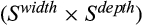
Solution quality. The solution quality of the GA methods compared to the optimal solutions is shown in Figure 6. The boxplots show that the median is 100% in all three variants. Additionally, the data evaluation reveals that the average solution quality exceeds 99% in all cases. The first quantile is equal to 100% for the WS, and is greater than 97% for the TS as well as the RS.

Figure 6

Solution Quality of Different Selection Operations in Comparison to the Exact Solution [Color figure can be viewed at wileyonlinelibrary.com]

In reference to the solution quality, the WS is slightly better than the TS and the TS is slightly better than the RS. To figure out what selection method is better suited for more extensive problem settings the execution time as a ratio of the solution quality achieved is examined more precisely. Problems five and six of Table 8 are considered which together consist of 200 problem instances. Figure 7 shows the median solution quality of the best individual solutions achieved up until the time shown on the x‐axis. The curve of the RS obviously increases more slowly than the curves of the other selection methods and the solution quality of the TS increases slightly faster compared to the WS. In conjunction with the results of Table 8 that have been discussed RS does not appear to be a suitable selection approach.

Figure 7

Median Solution Quality Depending on Execution Time [Color figure can be viewed at wileyonlinelibrary.com]

Summary. The results show that the median runtime for the FE increases exponentially as the number of items N and shelf space

S^{width} \times S^{depth}

increase. In comparison, the runtime of the GAs is lower and increases only very moderately. Furthermore, they achieved a close to optimal average solution quality of at least 99.1% in all three cases. In terms of runtime and solution quality, the TS is the most promising approach for larger problem settings. This is due to three facts. First, the runtime increase of the TS is lower compared to the other selection operations. Second, Table 8 shows that the TS has the shortest average computation times over all problem settings. Third, the median of the solution quality of TS is equal to WS, and the solution quality of TS compared to WS increases slightly faster.

Efficiency Analysis of Heuristics with Space Elasticity for Extensive Problem Settings

Three more extensive problem settings of practice‐relevant size are tested. The number of products and shelf space are increased in steps and the number of facings is increased to

K_{i} = 30

. The positive demand of an item has a uniform distribution within [1;30]. All other parameters are applied as above. The maximal runtime is bound to 500 seconds. Here we use the RSS and adapted start solution (ASS) which are described in section 4. The ASS uses the one‐dimensional solution of Hübner and Schaal (2017b).

Runtime. Table 9 once again shows that the TS is faster than the WS (GA WS vs. GA TS) for the smaller instances with 20 items. If the median runtime is close to the limit applied of 500 seconds, it means that in many cases the best solution has not yet been found due to the termination criteria. This means that the GA would still improve the solution with longer runtimes. This is the case for all GA WS applications and for the larger GA TS applications with 50 and 100 items. However, a significant runtime improvement can be obtained by applying the ASS. This makes it possible to obtain solutions within a few seconds, even for larger problems. Where the ASS TS has significantly shorter runtimes than the ASS RS.

Table 9

Median Runtime for Larger Problems, in seconds, 100 Instances, Rum Time Limit 500 seconds

Number of items N		20	50	100	Total
Total shelf space $S^{width} \times S^{depth}$		15×15	20×20	25×25	Total
GA WS	Median	430	412	466	441
GA TS	Median	117	480	482	466
GA ASS WS	Median	<1	2	5	2
GA ASS TS	Median	<1	1	3	1

Solution quality. There is no exact solution available that can be generated in reasonable computation time. We therefore use a benchmark. We use the solutions of the 1DSCASP

_{ex - prime}

problem which exclude non‐viable prime numbers but might be still an infeasible approach in terms of the arrangement options. Our calculations in Tables 6 and 7 allow the conclusion that the 1DSCASP

_{ex - prime}

is a suitable upper bound. For small instances, the gap compared to the 2DSCSP is 0.3% on average. Figure 8 shows the efficiency of the ASS methods. The ASS methods met the benchmark in almost all of the 300 test instances. The 300 test instances belong to the three test settings shown in Table 9 in ascending order of the problem size and are equally split (1–100, 101–200, and 201–300). The ASS TS method only missed the optimal solution in three cases. WS and TS with a RSS demonstrate much lower performance for the larger test instances (201–300), as here the solution quality suffers from a deficit in runtime.

Summary. The FE only has acceptable runtimes for very small problem sizes. This means it is not an appropriate procedure for real‐world problems. The GA configured with the selection operation WS and TS performs well for small and medium problem sizes. For more extensive problem settings, the GA with a RSS also leads to unsuitable runtimes. The increasing number of products and larger shelf space generate higher degrees of freedom. This results in greater opportunities for allocating the optimal item quantities onto the shelf space. As a result, the GA mostly only faces the prime number defects in more extensive problem settings, which makes the ASS an appropriate approach for solving them.

Efficiency of Heuristics with Space Elasticity and Substitutions

In this section, the model is extended by the substitution effects. To obtain a first indication that the GA is suitable to account for substitution effects, GA TS and GA ASS TS are compared to the heuristic approach AMIOAS (Algorithm for Mixed‐Integer Optimization of Assortment‐ and Shelf‐space problems) of Hübner and Schaal (2017a). Since this approach is only appropriate for the 1DSCASP with substitution, the GA is also applied to this setting with large problem settings. A second comparison with the GA TS and the GA TS ASS is applied to the two‐dimensional problem.

Algorithm suitability test for substitution effects. Tables 10 and 11 summarize runtime and the solution quality of the GA TS for the 1DSCASP. The model of Hübner and Schaal (2017a) is therefore a special case as it only yields feasible one‐dimensional solutions as it does not take into account two‐dimensional shelf space. The median solution quality of GA TS compared to AMIOAS is 99.2% and ranges between 97% to 99.9%. Despite the higher runtime and slightly lower solution quality for most problem settings, the GA TS has demonstrated appropriate performance for addressing substitution effects.

Table 10

Runtime of GA TS for 1DSCASP, in seconds, 100 Instances

Number of items N	20	50	100	Total
Total shelf space $S^{width} \times S^{depth}$	225×1	400×1	625×1	Total
Average	535	1,208	2,153	1,301
Median	471	1,138	1,998	1,173
Min	120	441	1,773	119
Max	1,683	1,973	3,589	3,589

Table 11

Median Solution Quality GA TS vs. AMIOAS for 1DSCASP, 100 Instances

Number of items N	20	50	100	Total
Total shelf space $S^{width} \times S^{depth}$	225×1	400×1	625×1	Total
Average ¹	0.997	0.992	0.969	0.986
Median ¹	0.999	0.993	0.970	0.992
Min ¹	0.984	0.978	0.942	0.942
Max ¹	1.000	0.999	0.986	1.000

¹ Calculation: GA TS profit / AMIOAS profit

Algorithm with a refined start solution to meet substitution effects. Due to the fast convergence times of Hübner and Schaal (2017a)’s algorithm, we will use an adjusted version of ASS in which the AMIOAS results are used as a start solution. Table 12 presents the percentage variance of the solution quality between the GA TS ASS and the GA TS after the limited runtime of 1,000 seconds. It shows that the GA TS ASS has achieved a 15.7% higher median on average for the most extensive problem setting. The difference between the two approaches is in evidence with a closer look at the time at which the best solution was found. The average median time of the smallest problem setting in Table 10 is 471 seconds for the GA TS, compared to 11 seconds for the GA TS ASS.

Table 12

Profit Difference between GA TS ASS and GA TS for 2DSCASP, in %, 100 Instances

Number of items	20	50	100	Total
Total shelf space $S^{width} \times S^{depth}$	15×15	20×20	25×25	Total
Average	0.3	1.9	15.6	5.9
Median	0.3	1.8	15.7	1.8
Min	−1.2	−0.6	6.6	−1.2
Max	1.6	3.8	24.7	24.7

¹ Calculation: (AMIOAS / GA TS profit profit −1) × 100

Summary. The numerical results with the integration of substitution effects has shown that the heuristic developed is suitable for addressing these effects. The second analysis has shown that an intelligent start solution is advisable with substitution effects, too.

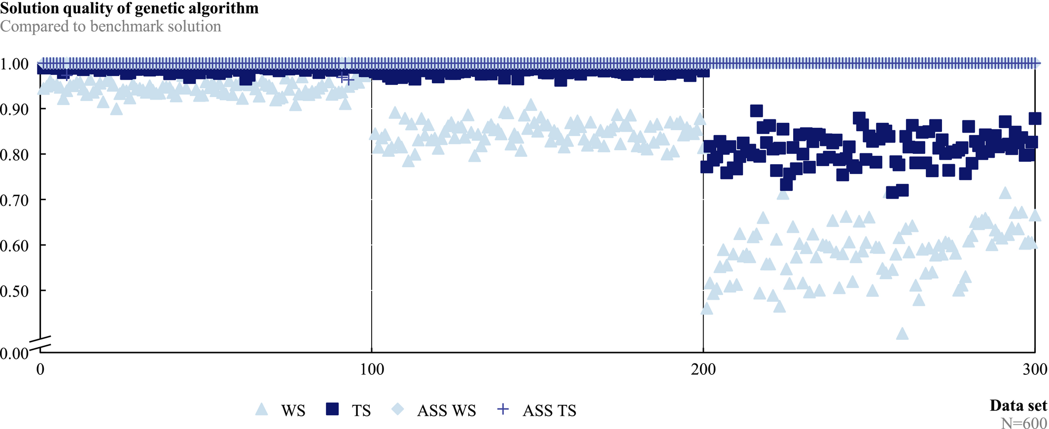
Effect of Combining Stochastic Demand, Space Elasticity, and Substitution

Because this is the first integrated stochastic model for two‐dimensional shelf spaces that accounts for space elasticity and substitution, this section illustrates the difference vis‐à‐vis the existing two‐dimensional model of Geismar et al. (2015) who do not account for demand effects. Total profits and shelf quantity assignments are compared. The parameters CV and β cover the values 0 and 0.35 with an interval of 0.05. The substitution rates considered range between 0 and 0.7 in 0.1 increments. All resulting combinations of the three parameters are evaluated. To investigate the impact of ignoring stochastic demand, space elasticity and/or substitution, a retailer is considered who makes assortment and facing decisions by assuming CV = β = λ = 0, while in reality there are CV > 0, β > 0 and λ > 0. To do so, we first run the model with CV = β = λ = 0 and evaluate ex post the results with the actual demand effects with CV > 0, β > 0 and λ > 0. This result is compared with an optimization run where the actual values of CV, β and λ are directly applied. This allows computing the impact of incorrect demand assumptions on assortment and facing decisions as well as the profit.

Figure 8

Profit Levels of GA Variants, in % of Benchmark Approach, Across all 300 Extensive Problem Settings [Color figure can be viewed at wileyonlinelibrary.com]

Figure 9 shows that the retailer gains up to 78% more profit on average (i.e., when β = 0.35, λ = 0.80 and CV = 0.35). Additionally, Figure 10 shows that up to 100% of all items get different facing quantities if stochastic demand, substitution, and space‐elasticity effects are correctly taken into account. It becomes clear that all three demand effects need to be considered jointly.

Figure 9

Profit Changes [Color figure can be viewed at wileyonlinelibrary.com]

Figure 10

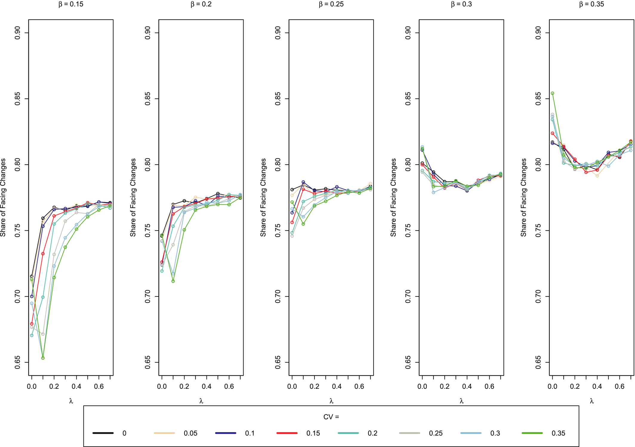
Share of Facing Changes [Color figure can be viewed at wileyonlinelibrary.com]

Case Study

After having shown that 2DSCASP can be efficiently solved to near‐optimal results within very short runtimes, it will be applied on a real data set in this section. The daily sales data of an assortment of 21 varieties of bread roll were collected at one of Germany’s largest retailers. Substitution rates between the items were identified using customer surveys. We interviewed n = 2,412 customers and asked them which substitute they would purchase if their first choice were unavailable. Asking customers whether the product they bought was really their first choice also captured substitute purchases for items that are actually unavailable. The substitution rates between two items i and j were then obtained by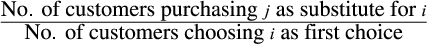

\frac{No. of customers purchasing j as substitute for i}{No. of customers choosing i as first choice}

. We had at least 30 interviewees for each item. Substitution rates per substitute amounted to up to 40% (see also Hübner and Schaal 2017a). The exact parameters are subject to confidentiality obligations. The minimum daily demand

δ_{i}^{\min}

varied between 1 and 25 units with a variation coefficient of

C V_{i} = [40 %; 152 %]

. Sales prices

r_{i}

ranged between

€ 1.5

and

€ 3.95

with unit costs of

c_{i} = [€ 0.32; € 1.02]

. The penalty costs

s_{i}

are set at zero. Because the items are perishable and our case study retailer has no further use for the items after the stated expiry date, the salvage value

v_{i}

is assumed to be zero. The retailer does not offer special discounts for items close to the expiry date. This is due to the short shelf life of bakery products (see also Kök and Fisher 2007 and Hübner et al. 2016 who analyze settings with no salvage values). Beyond the specific setting in our case study, we use non‐zero salvage values in the numerical analysis above to generalize our findings. To maintain a certain diversification on the shelf, the number of facings ranges between 1 and 30, whereby the shelf depth

S^{depth}

is 0.50m and the shelf width

S^{width}

is 1.20m. Currently, the retailer assigns shelf space to the 21 products based on sales proportions, that is, without explicit margins taken into account, demand volatility, space elasticity or substitution. The space elasticity β ranges in the sensitivity analysis between 0% and 30% in 5% increments. Additionally, 17% is added which is the average demand increase driven by space elasticity (Eisend 2014).

Table 13 shows the profit potential from applying our model. The retailer can increase profits by up to 15% depending on the assumed space elasticity. Furthermore, it can be seen that optimized assortments contain up to 38% fewer items than the current assortment. The increase in space elasticity leads to more shelf space for the most profitable items. This results in smaller assortments and an increasing number of items with facing changes.

Table 13

Results of Case Study

	Space elasticity β
	0%	5%	10%	15%	17%	20%	25%	30%
Profit potential¹	5.3%	5.6%	7.3%	8.1%	12.5%	11.2%	12.9%	14.8%
Assortment size²	86%	86%	81%	76%	71%	62%	62%	62%
Facing changes³	62%	67%	76%	81%	81%	86%	95%	95%
SD facing changes⁴	0.70	1.35	1.72	1.96	2.03	2.18	2.05	2.28

¹ Calculation: (2DSCASP profit / 2DSCASP

^{*}

profit)‐1

² Optimized assortment size as a share of current assortment size

³ Share of items with facings different to current facings

⁴ Standard deviation of absolute facing quantity changes

As a result of the remaining uncertainties of determining the parameters, we analyzed the profit potential together with the retailer depending on parameter robustness based on the average space elasticity of Eisend (2014). Moreover, we investigated the options for defining the appropriate shelf space for the bread roll category. We applied a sensitivity analysis for that purpose. To do this, the estimated substitution effects λ, variation coefficients CV and shelf space S are individually adjusted pro rata between 60% and 140% in 10% increments, whereas the other parameters remained unaffected. To ensure in‐store practicability, 20% increments are used for the shelf space. Table 14 shows that in a higher existing parameter ratio, substitution effects λ and shelf space S create more profit, whereby variation coefficients CV lead to decreasing profit. The following profit‐oriented managerial insights can be concluded for the retailer:

Table 14

Profit Potential Depending on Parameter Robustness

	Existing parameter ratio
	60%	70%	80%	90%	100%	110%	120%	130%	140%
λ	−4.2%	−3.0%	−2.0%	−0.6%	0.0%	0.7%	1.6%	2.5%	3.4%
CV	11.3%	8.9%	6.3%	3.3%	0.0%	−3.5%	−7.3%	−11.1%	−14.8%
S	−36.1%	–	−17.3%	–	0.0%	–	15.6%	–	27.7%

Inaccuracies in estimating the substitution effects have a slight impact on profit.

Slight deviations in determining the variation coefficients significantly affect profit.

If there is additional shelf space available, the retailer should enlarge the shelf space size for the bread roll category to increase profit.

Conclusion and Outlook

Conclusion Our model integrates assortment and shelf‐space optimization and takes into account stochastic demand, substitution and space elasticity. It supports retailers in creating a planogram for two‐dimensional shelves by determining optimal assortments and shelf quantities as well as the adjacently rectangular arrangement of each item’s facings. It is an integrated approach that simultaneously solves the four subproblems item selection, shelf quantity, facing arrangement, and item arrangement. Previous shelf planning literature focuses on regular shelf types where customers just see the foremost unit of an item. Solutions obtained for regular shelves cannot easily be transferred to two‐dimensional and tilted shelves. The combinatorial complexity of the model leads to a rapid increase in runtime with the number of items and the shelf‐space size. We developed a problem‐specific specialized heuristic that is based on a GA. In the numerical results we have shown that

one‐dimensional solution approaches of current literature are not readily appropriate methods for solving the two‐dimensional problems,

our algorithm efficiently yields near‐optimal results as our specialized heuristic achieves >99% of the exact approach on average for small instances,

neglecting stochastic demand, substitution and space elasticity leads to 78% lower profits and changes in facings of up to 85%, and

in a numerical analysis with the scope of one of Germany’s largest retailers, it may be possible to increase profits by up to 15%.

Future areas of research. Various opportunities exist for further research. Our model is based on several assumptions that could be relaxed in the future, e.g., we assumed that substitution takes place across one round only. Future models could account for several rounds of substitution, if substitutes are not available. The extension of our model is linked to the further development of solution approaches. Further heuristics can be developed to approach the stochastic nonlinear problem. Another topic of research interest is combination of the tactical problem described in this study with operational topics, such as shelf refilling, order management and inventory accuracy (cf. e.g., Curseu et al. 2009, DeHoratius and Raman 2008, DeHoratius and Ton 2015, Donselaar et al. 2010, Sharma et al. 2019, Xue et al. 2017). Further extensions in this area would address additional operational restrictions in backroom inventory and delivery frequency (cf. e.g., Eroglu et al. 2013, Holzapfel et al. 2016). Finally, the question of how a multi‐store environment can be taken into consideration requires investigation. For example, Bianchi‐Aguiar et al. (2015) developed an approach to replicate a standard planogram for several stores of a retail chain. A holistic multi‐store approach would also consider the potential impact of store segmentation on the efficiency of supply chain processes. The model and solution approach presented in this study has laid the foundation for these research questions.

References

Aastrup

Kotzab

. 2009. Analyzing out‐of‐stock in independent grocery stores: An empirical study. Int. J. Retail Distrib. Manag. 37(9): 765–789.

Agrawal

Smith

. 1996. Estimating negative binomial demand for retail inventory management with unobservable lost sales. Nav. Res. Logist. 43(6): 839–861.

Beasley

2004. A population heuristic for constrained two‐dimensional non‐guillotine cutting. Eur. J. Oper. Res. 156(3): 601–627.

Berlyne

D. E.

1958. The influence of complexity and novelty in visual figures on orienting responses. J. Exp. Psychol. 55(3): 289.

Bianchi‐Aguiar

Carravilla

M. A.

Oliveira

J. F.

. 2015. Replicating shelf space allocation solutions across retail stores. Working Paper, University Porto, 1–24.

Bianchi‐Aguiar

Silva

Guimaraes

Carravilla

M. A.

Oliveira

J. F.

Amaral

J. G.

Liz

Lapela

. 2016. Using analytics to enhance a food retailer's shelf‐space management. Interfaces 46(5): 424–444.

Bianchi‐Aguiar

Hübner

Carravilla

M. A.

Oliveira

J. F.

. 2019. Retail shelf space planning problems: A comprehensive review and classification framework. Working Paper, University Porto, 1–30.

Bortfeldt

Winter

. 2009. A genetic algorithm for the two‐dimensional knapsack problem with rectangular pieces. Int. Trans. Oper. Res. 16(6): 685–713.

Brown

W. M.

Tucker

W. T.

. 1961. The marketing center: Vanishing shelf space. Atlanta Econ. Rev. 9: 9–13.

10.

Campo

Gijsbrechts

Nisol

. 2004. Dynamics in consumer response to product unavailability: Do stock‐out reactions signal response to permanent assortment reductions? The influence of culture on services. J. Bus. Res. 57(8): 834–843.

11.

Chandon

Hutchinson

W. J.

Bradlow

E. T.

Young

S. H.

. 2009. Does in‐store marketing work? Effects of the number and position of shelf facings on brand attention and evaluation at the point of purchase. J. Mark. 73: 1–17.

12.

Corstjens

Doyle

. 1981. A model for optimizing retail space allocations. Management Sci. 27(7): 822–833.

13.

Curhan

R. C.

1972. The relationship between shelf space and unit sales in supermarkets. J. Mark. Res. 9(4): 406–412.

14.

Curseu

van Woensel

Fransoo

van Donselaar

Broekmeulen

. 2009. Modelling handling operations in grocery retail stores: An empirical analysis. J.Oper. Res. Soc. 60(2): 200–214.

15.

DeHoratius

Raman

. 2008. Inventory record inaccuracy: An empirical analysis. Management Sci. 54(4): 627–641.

16.

DeHoratius

Ton

. 2015. The role of execution in managing product availability. Agrawal

Smith

S. A.

, eds. Retail Supply Chain Management. International Series in Operations Research and Management Science. Springer, Boston, MA, USA, 53–77.

17.

Desmet

Renaudin

. 1998. Estimation of product category sales responsiveness to allocated shelf space. Int. J. Res. Mark. 15(5): 443–457.

18.

Donselaar

K. H. V.

Gaur

Woensel

T. V.

Broekmeulen

R. A.

Fransoo

J. C.

. 2010. Ordering behavior in retail stores and implications for automated replenishment. Management Sci. 56(5): 766–784.

19.

Drèze

Hoch

S. J.

Purk

M. E.

. 1994. Shelf management and space elasticity. J. Retail. 70(4): 301–326.

20.

Düsterhöft

Hübner

Schaal

K. N.

. 2019. A practical approach to the shelf‐space allocation and replenishment problem with heterogeneously sized shelves. Eur. J. Oper. Res. https://doi.org/10.1016/j.ejor.2019.09.012

21.

EHI Retail Institute . 2014. Retail data 2014: Structure, key figures and profiles of international retailing. EHI Retail Institute, Köln.

22.

Eisend

2014. Shelf space elasticity: A meta‐analysis. J. Retail. 90: 168–181.

23.

Eltze

Goergens

Loury

. 2013. Grocery store operations: Which improvements matter most? Akzente 1(1): 74–81.

24.

Eroglu

Williams

B. D.

Waller

M. A.

. 2013. The backroom effect in retail operations. Prod. Oper. Manag. 22(4): 915–923.

25.

Frank

R. E.

Massy

W. F.

. 1970. Shelf position and space effects on sales. J. Mark. Res. 7(1): 59–66.

26.

Gaur

Honhon

. 2006. Assortment planning and inventory decisions under a locational choice model. Management Sci. 52: 1528–1543.

27.

Geismar

H. N.

Dawande

Murthi

B. P.

Sriskandarajah

. 2015. Maximizing revenue through two–dimensional shelf–space allocation. Prod. Oper. Manag. 24: 1148–1163.

28.

Gilland

W. G.

Heese

H. S.

. 2013. Sequence matters: Shelf–space allocation under dynamic customer–driven substitution. Prod. Oper. Manag. 22(4): 875–887.

29.

Gruen

W. T.

Corsten

Bharadwaj

. 2002. Retail out‐of‐stocks: A worldwide examination of extent, causes and consumer responses: Report. Grocery Manufacturers of America, Washingtion and D.C.

30.

Hansen

Heinsbroek

. 1979. Product selection and space allocation in supermarkets. Eur. J. Oper. Res. 3(6): 474–484.

31.

Hansen

J. M.

Raut

Swami

. 2010. Retail shelf allocation: A comparative analysis of heuristic and meta‐heuristic approaches. J. Retail. 86(1): 94–105.

32.

Holzapfel

Hübner

Kuhn

Sternbeck

. 2016. Delivery pattern and transportation planning in grocery retailing. Eur. J. Oper. Res. 252(252): 54–68.

33.

Hopper

Turton

. 2001. An empirical investigation of meta‐heuristic and heuristic algorithms for a 2d packing problem. Eur. J. Oper. Res. 128(1): 34–57.

34.

Hübner

2011. Retail Category Management: Decision Support Systems for Assortment, Shelf Space and Price Planning. Lecture Notes in Economic and Mathematical Systems. Springer, Heidelberg.

35.

Hübner

Kuhn

. 2012. Retail category management: A state‐of‐the‐art review of quantitative research and software applications in assortment and shelf space management. Omega 40(2): 199–209.

36.

Hübner

Schaal

. 2017a. An integrated assortment and shelf‐space optimization model with demand substitution and space‐elasticity effects. Eur. J. Oper. Res. 261(1): 302–316.

37.

Hübner

Schaal

. 2017b. A shelf‐space optimization model when demand is stochastic and space‐elastic. Omega 69: 139–154.

38.

Hübner

Kuhn

Sternbeck

M. G.

. 2013a. Demand and supply chain planning in grocery retail: An operations planning framework. Int. J. Retail Distrib. Manag. 41(7): 512–530.

39.

Hübner

Kuhn

Sternbeck

M. G.

. 2013b. Retail operations: Why and how retailers benefit from an integrative supply chain management perspective. Wimmer

Hucke

eds. Inspiration, Ideas, Innovation. DVV Media Group, Hamburg, 359–439.

40.

Hübner

Kühn

Kuhn

. 2016. An efficient algorithm for capacitated assortment planning with stochastic demand and substitution. Eur. J. Oper. Res. 250(250): 505–520.

41.

Irion

J.‐C.

Al‐Khayyal

Tsao

Y.‐C.

. 2012. A piecewise linearization framework for retail shelf space management models. Eur. J. Oper. Res. 222(1): 122–136.

42.

Keijzer

Merelo

J. J.

Romero

Schoenauer

. 2002. Evolving objects: A general purpose evolutionary computation library. In: Lecture Notes in Computer Science. Springer Nature, Berlin, 231–242.

43.

Kellerer

Pferschy

Pisinger

. 2004. Knapsack Problems. Springer, Berlin.

44.

Kök

G. A.

Fisher

M. L.

. 2007. Demand estimation and assortment optimization under substitution: Methodology and application. Oper. Res. 55(6): 1001–1021.

45.

Kök

Fisher

M. L.

Vaidyanathan

. 2015. Assortment planning: Review of literature and industry practice. Agrawal

Smith

S. A.

, eds. Retail Supply Chain Management. Vol. 223 of International Series in Operations Research & Management Science. Springer, Boston, MA, USA, 175–236.

46.

Krishnamoorthy

C. S.

Venkatesh

P. P.

Sudarshan

. 2002. Object‐oriented framework for genetic algorithms with application to space truss optimization. J. Comput. Civil Eng. 16(1): 66–75.

47.

Lim

Rodrigues

Zhang

. 2004. Metaheuristics with local search techniques for retail shelf‐space optimization. Management Sci. 50(1): 117–131.

48.

Lodi

Martello

Vigo

. 1999. Heuristic and metaheuristic approaches for a class of two‐dimensional bin packing problems. Informs J. Comput. 11: 345–357.

49.

Martínez‐de Albéniz

Roels

. 2011. Competing for shelf space. Prod. Oper. Manag. 20(1): 32–46.

50.

Nielsen

A. C.

2004. Consumer‐Centric Category Management: How to Increase Profits by Managing Categories Based on Consumer Needs John Wiley & Sons, Inc., New Jersey.

51.

Pieters

Wedel

Batra

. 2010. The stopping power of advertising: Measures and effects of visual complexity. J. Mark. 74(5): 48–60.

52.

Pisinger

2005. Where are the hard knapsack problems? Comput. Oper. Res. 32(9): 2271–2284.

53.

Pisinger

Sigurd

, 2007. Using decomposition techniques and constraint programming for solving the two‐dimensional bin‐packing problem. INFORMS J. Comput. 19(1): 36–51.

54.

Rajaram

Tang

C. S.

. 2001. The impact of product substitution on retail merchandising. Eur. J. Oper. Res. 135(3): 582–601.

55.

Reiner

Teller

Kotzab

. 2012. Analyzing the efficient execution on in‐store logistics processes in grocery retailing – the case of dairy products. Prod. Oper. Manag. 22(4): 924–939.

56.

Ryzin

G. v.

Mahajan

. 1999. On the relationship between inventory costs and variety benefits in retail assortments. Management Sci. 45: 1496–1509.

57.

Schaal

Hübner

. 2018. When does cross‐space elasticity matter in shelf‐space planning? A decision analytics approach. Omega 244: 135–152.

58.

Sharma

Abouee‐Mehrizi

Sartor

. 2019. Inventory management under storage and order restrictions. Prod. Oper. Manag. https://doi.org/10.1111/poms.13097

59.

Smith

S. A.

Agrawal

. 2000. Management of multi‐item retail inventory systems with demand substitution. Oper. Res. 48(1): 50–64.

60.

Tan

Karabati

. 2013. Retail inventory management with stock‐out based dynamic demand substitution. Int. J. Prod. Econ. 145(1): 78–87.

61.

Urban

T. L.

1998. An inventory‐theoretic approach to product assortment and shelf‐space allocation. J. Retail. 74(1): 15–35.

62.

Wäscher

Haußner

Schumann

. 2007. An improved typology of cutting and packing problems. Eur. J. Oper. Res. 183(3): 1109–1130.

63.

Xue

Caliskan Demirag

Chen

F. Y.

Yang

. 2017. Managing retail shelf and backroom inventories when demand depends on the shelf‐stock level. Prod. Oper. Manag. 26(9): 1685–1704.

64.

Zhang

Wong

. 2015. An object‐coding genetic algorithm for integrated process planning and scheduling. Eur. J. Oper. Res. 244(2): 434–444.

65.

Zufryden

F. S.

1986. A dynamic programming approach for product selection and supermarket shelf‐space allocation. J. Oper. Res. Soc. 37(4): 413–422.