Multi-dimensional couple bargaining and housework allocation

Abstract

Research on couple bargaining and housework allocation focuses almost exclusively on partners’ economic resources. In this study, we ask whether additional bargaining resources, namely physical appearance and social networks, may exert a distinct effect – that is, whether partners can mobilize multiple resources within their bargaining framework. A focus on multiple bargaining chips is made possible by the German Socio-Economic Panel Study. In line with previous research, we conclude that earnings potential is the most important bargaining chip. But we also find that physical attractiveness can make a significant difference, although its effects depend on age. We uncover no distinct effects for social networks.

Keywords

Housework couple bargaining bargaining power earnings potential attractiveness social networks

Introduction

There is now a sizable literature addressing the gendered division of housework (Altintas and Sullivan, 2016; Coverman, 1985; Crompton, 1999; Bianchi et al., 2000, 2012; Bittman et al., 2003; Cooke, 2006; England, 2011; Esping-Andersen, 2009; Evertsson and Nermo, 2007; Killewald and Gough, 2010; Noonan, 2013; Sullivan, 2011; Sullivan and Gershuny, 2016). Mostly, the key question is whether men increase their share as women’s employment increases. Virtually all studies that rely on bargaining approaches identify bargaining power through partners’ economic capital, their earnings capacity in particular. The present study seeks to broaden our understanding of couple bargaining by including additional potential bargaining assets. We contribute specifically to household bargaining theory by extending our perspective beyond economic assets. It is doubtful that individuals, when asserting their preferences in cooperative bargaining settings, rely exclusively on income. Indeed, it is quite surprising that previous research has never explored the relative influence of additional resources.

Our core question is whether alternative resources can be mobilized when partners bargain over routine domestic tasks such as cleaning, washing and cooking. In addition to their respective economic resources, we also include the partners’ social networks (number of friends) and their physical attractiveness, measured via body mass index (BMI) data, as potential bargaining chips. We discuss several empirical and experimental studies, which suggest that the weight–height relationship of the BMI may serve as a proxy for individual attractiveness. Profiting from the longitudinal data of the German Socio-Economic Panel (SOEP) Study, we can (as did Evertsson and Nermo (2007) for Sweden, and Sullivan and Gershuny (2016) for the UK) examine how changes in bargaining resources affect changes in housework allocation in Germany. Germany poses an interesting case since a significant rise in female labor market participation occurs in the context of rather traditional gender norms. Increases in female work have been mostly part-time, and a modified male breadwinner model remains the dominant model, particularly in the West. In such a context, it remains unclear whether female earnings power affects housework bargaining as input or outcome (Ott, 1995). Alternative bargaining indicators, such as those we propose in this study, might provide further insights as they should not provoke such ambiguities of causality direction. From a more general perspective, we hope our study will spark further research on couple bargaining that explores the idea of alternative forms of bargaining power beyond the classic income indicator.

Theoretical framework

Explicitly or implicitly, most studies adopt a bargaining perspective when examining how the partners’ resources influence the division of domestic work. The basic premise in most studies is a Nash bargaining model with a cooperative equilibrium (Nash, 1953; Pollak, 2005). This implies that the partners cooperate to maximize joint welfare, but also wish to promote their own distinct preferences. The joint utility of domestic production is a clean home, tasty meals, and so on. One would assume that individuals will prioritize other activities, be they leisure, childcare or paid work, while minimizing their contribution to housework tasks.

Bargaining models also assume that each partner will have a distinct threat point (Lundberg and Pollak, 2007; McElroy and Horney, 1981; Manser and Brown, 1980). The latter will depend on one’s bargaining resources – that is, stronger bargaining power results in a better position to assert individual preferences. Both partners’ threat points determine where the equilibrium solution rests, or, in other words, what arrangement they can agree on. If one partner disregards what his or her significant other can demand on the basis of his/her bargaining power, this violates the other one’s threat-point, and he or she will abstain from bargaining altogether. In some studies this is argued to lead to partnership breakdown or divorce (Lundberg and Pollak, 2007). However, the implicit determinism of these divorce-threat models led Lundberg and Pollak (1993) to develop an alternative ‘separate spheres’ model where exceeding the threat-point results instead in a non-cooperative bargaining dynamic (Nash, 1951).

Gender roles and housework bargaining

As noted, the literature almost exclusively considers bargaining power in the form of economic resources. A key question is, whether ongoing changes in women’s economic role translate into less gendered domestic behavior. Most studies find that any increase in her bargaining power results in a decrease in her relative housework input; in parallel, men’s contribution tends to increase less than one would predict (Bittman et al., 2003; Breen and Cooke, 2005; Brines, 1994; Brodmann et al., 2007; Evertsson and Nermo, 2004, 2007; Greenstein, 2000; Gupta, 2007; Parkman, 2004; Prince Cooke, 2006; Sullivan, 2011; Sullivan and Gershuny, 2016).

This suggests that women do not profit from a given level of income to the same extent as men do. In some studies, this outcome is interpreted as conformity to expected gender norms (Cooke, 2006). The ‘gender deviance neutralization thesis’ (Bittman et al., 2003) has, however, received only scant empirical support, and most recent studies find little evidence in its favor. Evertsson and Nermo (2004, 2007) found some evidence of adhering to such gender norm practices in the US, but not in Sweden. Sullivan (2011) and Sullivan and Gershuny (2016) find basically no evidence of it in Britain. Nevertheless, any empirical approach to couple bargaining requires us to take into account the biasing impact of prevailing gender norms.

Economic bargaining resources

The majority of studies measure bargaining capacity with income indicators (Chen and Woolley, 2001; Lundberg and Pollak, 1996; Manser and Brown, 1980), earnings potential (Bielby and Bielby, 1992) or, as Pollak (2005), with wages (for an overview, see Doss, 2013). Most use a relative measure, such as the gap between the partners’ earnings. Gupta (2007), however, found that the inclusion of an absolute earnings measure seriously weakens the impact of relative earnings shares. He concluded that absolute and relative resources capture two distinct phenomena. The former measure the degree of economic independence – that is, whether any of the partners can manage on their own in a post-divorce situation; the relative measure defines how strong a partner’s bargaining position is compared to the other’s. That said, it is possible that men and women utilize different kinds of resources and weigh their specific impact against each other. It is for this reason that we choose to extend the realm of resources to also include attractiveness and social networks.

We shall consider the influence of both absolute and relative economic resources. A woman with high earnings can be considered economically independent even if the partner’s income clearly exceeds hers (Gupta, 2007; Gupta and Ash, 2008). An unclear issue is how to treat couples with an economically inactive spouse when estimating bargaining effects. Gupta (2007), Killewald and Gough (2010) and Gough and Killewald (2011) exclude such couples from their analyses. In Germany, where many couples still adhere to a (modified) male breadwinner model, this would imply a limited ability to generalize the findings. The alternative of assigning a zero income implies that the homemaker has no economic bargaining power at all. This is unrealistic, given that individuals usually can rely on a minimum of work income after separation, even if they did not work before the split-up (Pollak, 2005). Sullivan and Gershuny (2016) propose an approach that derives economic bargaining power from predicted wages (i.e. wage potential). This provides an excellent solution to the problem, and we shall follow this approach for absolute and relative earnings power.

Social networks as a bargaining resource

Bargaining theory has so far focused on the structural positions within social networks as a determinant of bargaining power (Braun and Gautschi, 2006). Here we pursue an individual perspective, viewing the ability to rely on a social network as social capital (Coleman, 1988; Lin, 2017), and as a potential bargaining resource. Having an extensive social network can significantly contribute to the quality of a couple’s social life, and may also further the career prospects of the partners – the strength of weak ties (Granovetter, 1973). Moreover, employment tends to extend social networks. Here, bargaining power increases in tandem with the level of social and economic autonomy (Doss, 2013). The idea we pursue here is that embeddedness in a social network provides access to exchange resources, which should improve the bargaining position within couples. Individuals tend to rebuild their social life in order to compensate for the loss of a spouse (Kalmijn and van Groenou, 2005).

The ability to rely on generalized (i.e. collective, trusting and flexible) forms of exchange in a social network may constitute a bargaining resource in its own right (Uehara, 1990) that compensates for the loss of spousal resources. And a strong social network might influence the threat-point, since reliable friends can provide emotional and other forms of support in case of separation, thus cushioning the effects of a split-up (Allan, 2008; Walen and Lachman, 2000). This might arguably increase one’s relative bargaining position by diminishing the other partner’s divorce threat in a threat-point model. Additionally, strong social networks can augment one’s bargaining power if, in a potential divorce scenario, the other partner will face adverse consequences, be they in the form of loss of social integration, or earnings and career prospects. Network research also suggests that it is not only the size of a social network that matters, but also the nature and type of relations: close kinship networks and generalized trusting friendship ties promise more generous support than restricted (i.e. more competitive, less trusting) networks (Uehara, 1990). However, when interpreting the reliance on network resources, we should keep in mind that they are less tangible than economic resources (Blau, 1964). Income functions by improving outside options after separation, but may also be exchanged to improve the well-being of one’s significant other. In contrast to this dualistic nature of economic resources, expected support from social networks is limited in its transferability, which may considerably hamper its role as power in couple bargaining.

Physical attractiveness as a bargaining resource

Experimental research suggests that physical attractiveness may affect social relations in the form of a beauty premium (Ravina, 2008; Rosenblat, 2008; Solnick and Schweitzer, 1999). We interpret this as a resource that improves chances in the partnering-market, and, once partnered, it is a potential form of bargaining power. If the partners favor attractiveness in their significant other, they may be more disposed to heed to the other’s wishes and preferences. Additionally, attractiveness can influence the threat point because it can be a post-divorce asset in the sense that the attractive person will re-enter the marriage market with a desirable asset.

Two major – and, in part, conflicting – premises dominate the theoretical discussion on this subject. First, attractiveness homogamy in mate selection appears to be prevalent (Carmalt et al., 2008; McPherson et al., 2001). Second, the idea of ‘beauty exchange’ (the ‘trophy wife’), where women trade beauty for men’s social status, has received much scholarly attention (Elder, 1969; Gullickson, 2017), but has recently been challenged on the basis of methodological shortcomings of previous research (McClintock, 2014). For developing theoretically guided hypotheses, the homogamy perspective poses difficulties. If women prefer a handsome male, men might also be able to utilize this as a resource in household bargaining. But if physical appearance functions as bargaining power, and both men and women have a similar command over this resource, neither should receive a bargaining advantage. The idea of a female beauty premium is more straightforward. Where physical appeal is exclusively a female asset, this introduces an aspect of asymmetry into gender-related bargaining power, where men and woman cannot utilize a specific resource to the same extent.

Of course, we do not have any information that captures beauty directly. However, there is solid evidence that physical appearance in the form of weight, height or their correlates in the form of BMI are closely related to peoples’ assessment of attractiveness (Carmalt et al., 2008; McClintock, 2014; Tovée et al., 1998, 1999a, 1999b). These findings also suggest the salience of culturally shaped perceptions of desirable weight–height relations (Swami and Tovée, 2005), as the BMI perceived as most attractive is biased towards lower values for women (with a mean around 20) than for men (around 22) (Tovee and Cornelissen, 1999; Tovée et al., 1998).

While these studies refer to attractiveness as a concept, we are aware that while beauty lies in the eye of the beholder, these BMI transformations only capture a very specific aspect of looks in the form of physical appearance. In the following, our discussion of attractiveness refers exclusively to physical appearance.

Our study must be viewed as explorative because this is the first sociological attempt to estimate the combined influence of physical appearance, social networks and economic resources on partnership bargaining. It is, therefore, difficult to develop strong, theoretically guided hypotheses. We can, nonetheless, offer some cautionary hypotheses.

In general, we assume that receiving higher earnings, being more attractive and having a larger social network decreases one’s share of housework. Additionally, we propose three more specific hypotheses. Firstly, based on prevalent gender-role ascriptions, we expect that the influence of physical appearance should be more decisive for women (Carmalt et al., 2008). We also predict that this bargaining effect declines significantly by age (England and McClintock, 2009).

Secondly, predictions regarding the bargaining impact of social networks are difficult to make since we have no information on the kinship ties and the nature of friendship networks involved. We can only identify the sheer number of close friends (see Data and Methods section). Had we been able to identify the kinds of relationships within the network, we would be in a far better position to make predictions (Uehara, 1990).

Thirdly, taking into account the standard finding that economic resources dominate bargaining power, we expect these to remain decisive even when taking also networks and attraction into consideration.

Data and methods

In our study, we analyze the German SOEP Study (Wagner et al., 2007). Starting in 1984, this representative household panel surveys around 13,000 German households, providing information on a broad variety of socio-economic characteristics for both individuals and couples. Decisively, it includes annual data on the distribution of housework for both partners.

We draw on data from the 2002 to 2015 waves (some of the data, central to our analyses, such as individuals’ weight and height, were not collected prior to 2002). We focus on the core samples, and restrict our analyses to men and women aged 20–40 in different-sex couples. The rationale is to investigate couple behavior in the division of domestic labor in a life-course stage during which conflicts between domestic and market work are most likely.

We also apply a cohort-based restriction, focusing on individuals born between 1963 and 1988. This combines a sufficient degree of similarity within the cohorts considered with a sufficient number of observations. Furthermore, we restrict the analysis to couples who have been living together for at least two successive years to make sure they have already established a basic routine regarding their division of housework. The analyses are based on a semi-balanced panel with at least two successive waves of survey participation.

Model design and dependent variables

We measure core housework hours during a normal weekday. The survey question is phrased as follows: ‘How many hours do you spend on the following activities on a typical weekday?’ – item: ‘housework (washing, cooking, cleaning)’. Although such responses are less precise than information derived from time-use surveys, they are generally considered a suitable approximation of routine activities (Brines and Joyner, 1999).

We deliberately adopt a focus on doing laundry, cooking and cleaning since these represent the most time-intense and tedious domestic duties, which are still primarily done by women (Gupta, 2007). Activities like doing errands or household repairs are associated with larger male contributions, and they are typically less time-consuming and more pleasant than cleaning (Bianchi et al., 2000).

The dependent variable is the partners’ relative share of housework hours on an average weekday. The relative measures of our key independent variables – that is, wage potential, friends and attractiveness – are constructed in the same way as the relative share of housework with:

x_{p_{r e l}} = \frac{x_{p_{i n d i v i d u a l}}}{x_{p_{i n d i v i d u a l}} + x_{p_{p a r t n e r}}}

y_{h w_{r e l}} = \frac{y_{h w_{h o u r s_i n d i v i d u a l}}}{y_{h w_{h o u r s_i n d i v i d u a l}} + y_{h w_{h o u r s_p a r t n e r}}}

where x_prel represents the relative bargaining power (wage potential or attractiveness, equation (1)). This approach leads to a normalized scale ranging from 0 to 1 (with, from ego’s perspective, 0 displaying zero bargaining power, 0.5 displaying an even share of bargaining power between the partners and 1 implying that ego commands the total amount of bargaining power). The dependent variable relative housework share (hw_rel ), is calculated in the same manner (0 indicates no housework contributions from ego, while 1 indicates that she/he provides all housework in the couple; cf. equation (2)). The data on housework contributions, earnings and other indicators are collected from each partner’s individual survey responses – that is, we collect questionnaire data for each partner, and link them via a partner indicator provided in the SOEP. This approach ensures far greater accuracy than relying on proxy information on the partner’s contributions as other studies do.

We adopt two methodological approaches. The first is based on a set of pooled (including all panel waves from 2002 to 2015) ordinary least squares (OLS) regressions. We estimate with clustered, robust standard errors c_ig, with index g denoting the vector of repeated observations per individual. Model 1 (Table 1) is based on a joint model of male and female respondents, displaying interaction effects between sex and bargaining power indicators in order to identify whether men and women rely on the same resources in unburdening themselves of household duties.

Table 1.

Pooled OLS regression of husbands’ and wives’ relative share of housework (ages 20–40).

	(1) Base model	(2) Work controls	(3) Relative bargaining
	B/SE	B/SE	B/SE
Female	1.20***	1.067***	1.062***
	(0.015)	(0.014)	(0.014)
Wage potential (z, log)	–0.169***	–0.028**
	(0.011)	(0.010)
IA: female^*	–0.105***	–0.101***
Wage potential	(0.013)	(0.012)
Relative wage potential (z, log)			–0.104
Share of combined wages			(0.014)***
IA: female^*			–0.029^*
Relative wages			(0.011)
Few friends (0–1)	–0.020	–0.019	–0.016
vs more (y/n)	(0.017)	(0.017)	(0.017)
Attractiveness (z)	0.049***	0.043***
0 (low) to 5 (high)	(0.009)	(0.009)
IA: female^*	–0.065***	–0.056***
Individual attractiveness	(0.011)	(0.011)
Attractiveness (z)			–0.001
– partner relative			(0.008)
IA: female^*			0.004
Relative attractiveness			(0.011)
Economically inactive/marginal		1	1
Work (reference)
Part-time work		–0.121***	–0.108***
		(0.017)	(0.017)
Full-time work		–0.520***	–0.494***
		(0.016)	(0.016)
Partner not working	–0.477***	–0.462***	–0.312***
	(0.012)	(0.012)	(0.016)
Doctor visits during	–0.009^*	–0.007⁺	–0.008⁺
last three months (z, log)	(0.004)	(0.004)	(0.004)
Pre-school children?	0.032***	0.041***	0.047***
(y/n)	(0.010)	(0.009)	(0.010)
East Germany	–0.088***	–0.002	–0.022⁺
	(0.014)	(0.013)	(0.014)
Aged 30–40	0.099***	0.056***	0.037**
Ref. age < 30	(0.013)	(0.013)	(0.013)
Intercept	–0.649***	–0.183***	–0.189
	(0.011)	(0.025)	(0.033)
R ²	0.681	0.708	0.708
n of observations	27,957	27,957	27,957
n of individuals	6973	6973	6973

⁺ p < 0.1.

*p < 0.05.

**p < 0.01.

***p < 0.001.

Robust standard errors in parentheses.

Omitted controls: educational homogamy, cohort, migration background, sports activity level.

Note: effects for wage potential and attractiveness account for changes in one SD.

IA: interaction effects.

Source: SOEP 2002–2015, authors’ calculations.

y_{i t} = α + β_{p_{z}} x_{p_{z} i t} + β_{k} x_{k i t} + c_{i g}

In the second approach, we investigate changes in relative housework over time, applying fixed-effects estimations in order to test whether any increase in bargaining power between t–₁ and t₀ leads to a reduction in hourly housework at t₀.

y_{i t} = α + β_{p_{z}} x_{p_{z} i t} + β_{k} x_{k i t} + u_{i t} + ∊_{i t}

The equations (3) and (4) include model controls x_k as well as different indicators of bargaining power, x_p . The regression models denoted under (3) and (4) identify the impact of absolute bargaining power (i.e. the absolute wage potential independent of the partner’s) as well as relative measures for wage potential, networks and attractiveness.

Measuring bargaining resources

Following Sullivan and Gershuny (2016), we use net monthly wage potential to identify the partners’ absolute and relative economic power. We deliberately choose wages over income, since the latter also reflects the amount of working hours which, in turn, affects time availability (Coverman, 1985; Hook, 2010). However, we control for full-time (>30 hours), part-time (15–30 hours) and inactivity (<15 hours) in the model, since these distinguish basic degrees of labor market attachment.

We estimate the wage function based on the Mincer (1974) approach, and follow Heckman’s (1979) refinement, applying a two-step estimator. First, we estimate an OLS regression wage function (detailed estimates available on request), based on the characteristics of those employed and receiving a wage at t₀ with:

\begin{array}{l} y w a g e = α + β_{} s e x + β_{} r e g i o n + β_{} m i g r a n t + β_{} a g e + β_{} a g e s q + β_{} m a r r i e d \\ + β_{} n k i d s 06 + β_{} e d u c a t i o n + β_{} o c c p r e s t i g e + β_{} o c c p r e s t i g e s q \\ + β_{} f u l l t i m e x p + β_{} u n e m p l x p + β_{} e m p s t a t u s_{t - 3; t - 1} + β_{} w a g e s_{t - 3; t - 1} \end{array}

This estimator (equation (5)) constitutes the basis for an individual’s wage potential used in equations (3) and (4).

We test whether housework contributions differ between individuals with a very thin as opposed to a dense social network. The bargaining effect of social networks is, however, unlikely to increase linearly with the number of friends. Hence, we distinguish via a dummy indicator those who can rely on a moderate to large friendship network from those who are relatively isolated with only one or no close friends at all.

The number of close friends was collected in 2–5-year intervals since 2003 in the SOEP. This should provide sufficient variation of observation given the relative stability of friendship networks.

Measuring attractiveness as bargaining power

Relying on Tovée et al. (1998, 1999a, 1999b), we use a transformation of the BMI to assess physical appearance. The subjects in the Tovée et al. experiments were shown photographs of real persons in order to rate their attractiveness. These ratings were then integrated into a distribution of beauty ratings across BMI, which were recorded along with the visual display, but not disseminated to the test subjects. The ratings resulted in a slightly right-skewed normal distribution, peaking around an ideal BMI.

We mimic this distribution based on the BMI in our sample with the following procedure: we first calculate a respondent’s distance from what was perceived as the most attractive BMI in the Tovée studies (between 21.5 and 22.5 for men, and 19.5 and 20.5 for women). As the scale range for over- and underweight differs, we apply a logarithmic function for BMI values that deviates towards overweight. This is based on the idea that additional BMI unit changes in the realm of extreme obesity only have a marginal impact on further changes in attractiveness. Secondly, we assign a continuous 0–5 score based on the individual log-distance to the most attractive BMI, where a higher score depicts more attractiveness. For the fixed-effects estimations, we additionally include an indicator that distinguishes whether an individual lost weight since t-2, improving their BMI from a value near obesity to over- or normal weight (i.e. from ≥ 28 to ≤ 26).

We include height in our indicator, since specific height ranges are perceived as more attractive (Pierce, 1996). Research suggests that the ideal height is slightly above 1.80 m for men, and around 1.65 m for women (Buss, 2008; Stulp et al., 2013). A height around these values may also signal good health and fertility (Stulp and Barrett, 2016). Outliers receive penalties for limited attractiveness (Graziano et al., 1978). We implement a height-based correction of our BMI attractiveness score with a factor between 1 (for close to ideal height) to 0.8 (for extreme outliers). Details on height correction and sensitivity tests for alternative height-based adjustments are available on request.

We bear in mind that there are other conditions that may affect the weight component of the BMI, but do not affect attractiveness, or which affect both weight and time available for housework. We include the (log) number of doctor visits within the last quarter to identify possible health problems that might limit a partners’ ability to perform housework tasks, while simultaneously affecting weight. Initially, we considered obesity to differentiate attractiveness from health-based aspects of the BMI. We excluded this control in the final models due to insignificance and co-linearity, favoring, instead, the more general health indicator of doctor visits. Additionally, we consider the intensity of sports activities, assigning a score for whether an individual does sports regularly or more rarely. Frequent sports activity will likely reduce time available for household tasks, while simultaneously affecting weight. We consider whether a woman was pregnant at the time of a given interview and the pregnancy month. Since pregnancy will likely affect both weight and activity levels in later months, while not necessarily affecting attractiveness, we control for the number of pregnancy months beyond month five.

Additional model controls

Additional controls include educational homogamy for those with university-level education, since such couples tend to display a more egalitarian division of domestic work. We exclude educational attainment, as it is highly correlated with wage potential, and none of our estimations yield a significant education effect on housework after controlling for relative wage potential.

Further controls include, firstly, a dummy for growing up in East or West Germany. The stronger employment attachment of East German women has translated into different cultures in the division of housework (Trappe et al., 2015). We control for migration background, since many of the first- and second-generation immigrants in Germany adhere to a more traditional division of labor. We also control for whether the partner is not working, since this may influence both power relations and time available for housework.

Additionally, we identify the presence of pre-school children, since this is likely to impose additional time constraints; having small children will probably also promote more traditional gender roles, certainly in Germany (Wengler et al., 2009). We distinguish between those born in the decades from the 1960s to the 1980s. This takes into account a more egalitarian division of labor within younger cohorts (England, 2011). By controlling for age, we introduce a life-course perspective associated with changing levels of housework intensity.

Empirical results

As displayed in Table 1, we estimate a pooled model of husbands’ and wives’ relative housework burdens. Here, we distinguish gender-specific effects by introducing interactions between sex and wage potential and attractiveness as indicators of bargaining power. This will serve as a frame of reference for our analyses. Firstly, women contribute considerably more to relative housework as a rule. This is by far the clearest outcome in all our analysis. It is additionally supported by the interaction effect estimates.

Among our bargaining power indicators, the (log) wage potential is by far the most decisive one. Model 1 focuses on the role of absolute resource endowments among men and women. Figure 1 provides a graphical display of this relationship. For both men and women, an increase in (log) wage potential results in a reduction of their share of housework. It is especially in the low-wage domain that women profit in terms of reducing relative housework in tandem with a wage increase. However, women’s share of housework remains higher than men’s across all segments of the wage distribution.

Figure 1.

Respondent’s share of joint housework – marginal effects of individual wage potential by sex (age 20–40). Number of observations = 27,957; number of individuals = 6973. Base model: Table 1(1).

We additionally control for full-time, part-time or economically inactive status in Table 1 (Model 2) in order to cleanse the wage indicator of time availability. A focus on hourly wages should – by design – be immune to mixing up effects of earnings and time availability. However, high-wage earners are also more likely to be in full-time occupations with more demanding time schedules. Recall that we deliberately exclude an exact measure of working time in order to avoid co-linearity. After controlling for employment status in Model 2, the relation between wage potential and the reduction in housework hours remains significant.

Figure 1 (based on Model 1 in Table 1) displays the common pattern of higher potential wages resulting in a lower share of housework. While women contribute a considerably larger share to joint housework, their decrease with a higher wage potential amounts to a similar size as among men.

Turning now to couples’ relative wage potential, we uncover a similar pattern (see Model 3 (Table 1) and Figure 2). An increase in one’s relative wage potential helps reduce housework among both men and women. However, gender differences persist, and women keep doing about half of the housework even when they are the sole breadwinner. An increase in her relative wage share from 0 to 100% is associated with a reduction of her housework share of about 25%. For him, the same change in wage potential results in a reduction of his housework share of about 50%. Interestingly, in the highest wage segments (earning >80% of joint wages), a further increase in wage potential does not produce any additional decline in housework among men or women. Figure 2 summarizes this effect with a cubic function.

Figure 2.

Respondent’s share of joint housework – marginal effects of relative wage potential by sex (age 20–40). Number of observations = 27,957; number of individuals = 6973. Base model: Table 1(3) with cubic function of relative wage potential (see equation (2) for calculation of relative wage potential).

The models in Table 2 examine the bargaining outcomes for women only. Their male partners are still considered implicitly in the calculation of relative housework, wages and attractiveness. The focus on women offers some further insights into processes behind the gender asymmetries in housework: having pre-school children is associated with a clear increase in women’s relative housework share (see Table 2). This can be seen as a manifestation of Germany’s traditional gender roles.

Table 2.

Pooled OLS regression of wives’ relative share of housework (ages 20–40).

	(1) Base model	(2) Work controls
	B/SE	B/SE
Wage potential (z)	–0.083***	–0.076***
	(0.016)	(0.015)
Relative wage potential (z)	–0.227***	–0.056***
share of couple’s combined wages	(0.013)	(0.013)
Few friends (0–1)	0.019	0.022
vs more (y/n)	(0.021)	(0.021)
Attractiveness (z)	–0.021^*	–0.019^*
0 (low) to 5 (high)	(0.009)	(0.08)
Attractiveness (z)	0.020^*	0.021^*
– partner relative	(0.010)	(0.09)
Inactive/marginal work (reference)		1
Part-time work		–0.170***
		(0.017)
Full-time work		–0.525***
		(0.018)
Partner not working		–0.317
		(0.025)***
Doctor visits during	–0.025***	–0.022***
last three months (z, log)	(0.005)	(0.005)
Sports activity level	–0.016***	–0.017***
0 (low) to 5 (high)	(0.005)	(0.004)
Pregnant beyond	–0.025***	–0.017^*
month 5 (0–5)	(0.005)	(0.007)
Pre-school children?	0.142***	0.038***
(y/n)	(0.013)	(0.012)
Homogamy in college	–0.134***	–0.109***
Education	(0.021)	(0.019)
East Germany	–0.171***	–0.226***
	(0.017)	(0.028)
Intercept	0.529***	0.930***
	(0.025)	(0.027)
R ²	0.249	0.335
n of observations	15,912	15,912
n of individuals	3880	3880

⁺ p < 0.1.

*p < 0.05.

**p < 0.01.

***p < 0.001.

Robust standard errors in parentheses.

Omitted controls: cohort, age group, migration background.

Note: effects for wage potential and attractiveness account for changes in one SD.

Source: SOEP 2002–2015, authors’ calculations.

The second bargaining chip, namely social networks, appears to have no pronounced effect. None of the results in the pooled models (Tables 1 and 2) or the fixed-effects estimation (Table 3) provide any support for its influence. This could be due to our relatively rough measure, distinguishing between those with no network (0–1 close friends), and those with more friends. We also tested other measures of the number of friends (n-metric, or n-logged), but none yielded any significant impact (results available on request). Hence, our hypothesis that social networks (as measured here) constitute a bargaining chip is not supported.

Table 3.

Fixed-effects estimates of wives’ annual change in relative share of housework (ages 20–40).

	(1)	(2)	(3)
	B/SE	B/SE	B/SE
Wage potential (z)	–0.102*	–0.102*	–0.110
	(0.042)	(0.042)	(0.029)
Relative wage potential (z)	–0.198***	–0.197***
share of combined wages	(0.037)	(0.037)
Change in relative wages			–0.182***
since t_–1			(0.013)
Few friends (0–1)	–0.116	–0.120	–0.103
vs more (y/n)	(0.088)	(0.088)	(0.087)
Attractiveness (z)	0.008
0 (low) to 5 (high)	(0.046)
Drop in BMI from obesity		–0.046*	–0.045*
since t_–1		(0.023)	(0.023)
Economically inactive/marginal work (reference)	1	1
Part-time work	–0.321***	–0.272***
	(0.056)	(0.055)
Full-time work	–0.273***	–0.265***
	(0.055)	(0.058)
Not working to part-time			–0.442***
since t_–1			(0.063)
Not working to full-time			–0.373***
since t_–1			(0.065)
Partner not working	–0.273***	–0.275***
	(0.069)	(0.068)
Partner stopped working since t_–1			–0.281***(0.078)
Intercept	0.098	0.118	0.004
	(0.110)	(0.109)	(0.1)
R ²	0.030	0.030	0.055
n of observations	15,912	15,912	15,912
n of individuals	3880	3880	3880

⁺ p < 0.1.

*p < 0.05.

**p < 0.01.

***p < 0.001.

Omitted controls: cohort, age group, educational homogamy, doctor visits, sports activity, pregnancy, pre-school children.

Note: effects for wage potential and attractiveness account for changes in one SD.

Source: SOEP 2002–2015, authors’ calculations.

Attractiveness has, however, a significant effect on housework shares for men and women alike – but in different directions (see Table 1: Models 1 and 2): the woman’s (absolute) attractiveness helps reduce her housework share; in contrast, male attractiveness results in a greater contribution to joint housework. While the effect of the absolute measure of attractiveness is positive in the male and female joint model presented in Table 1, the introduction of a gender interaction shows that this is primarily the display of the (positive) male effect, while her attractiveness counters the male effect and tips the balance in the opposite direction – that is, for her, greater attractiveness implies relatively less housework, as illustrated in Figure 3.

Figure 3.

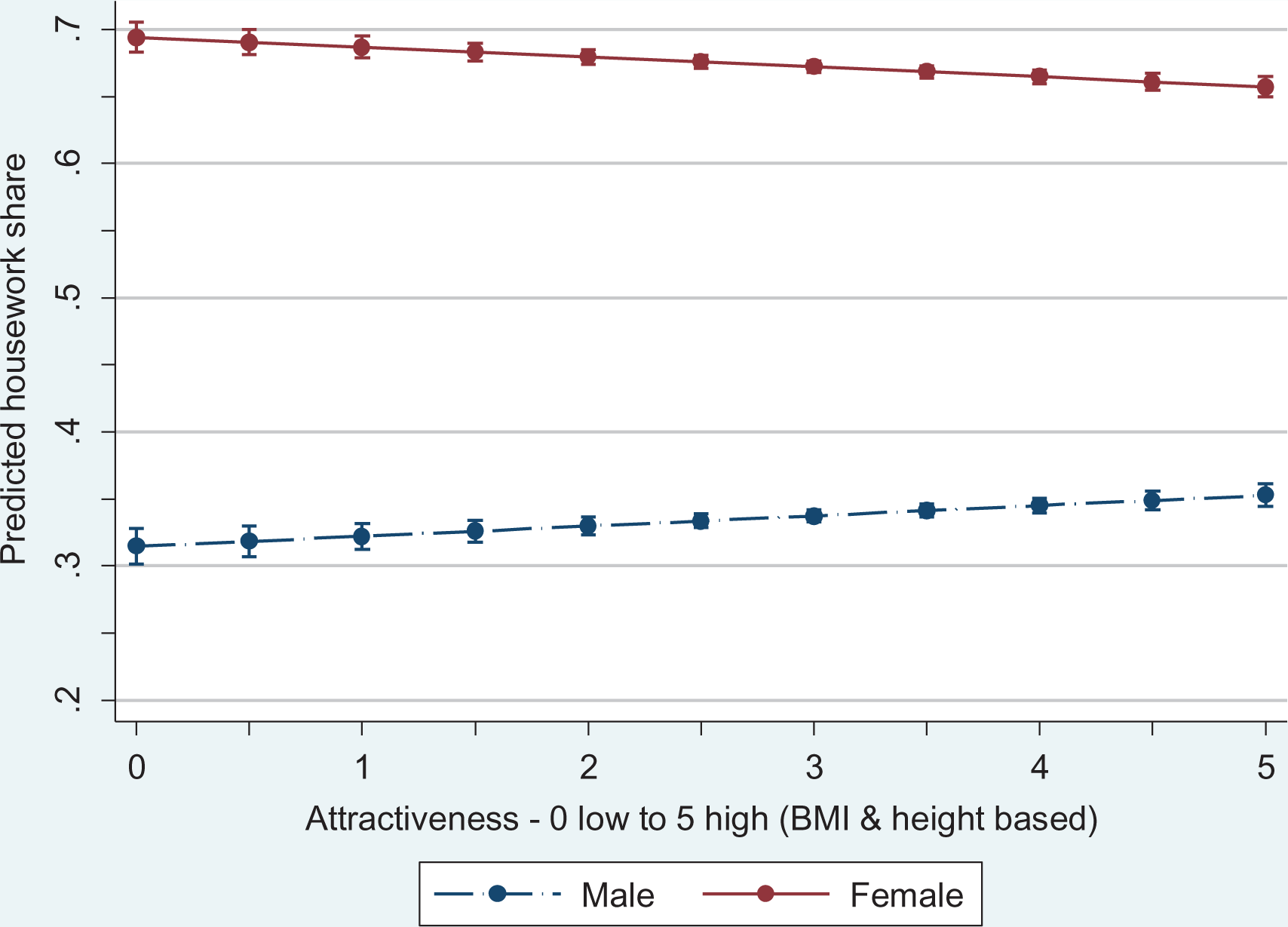
Respondent’s share of joint housework – marginal effects of attractiveness by sex (age 20–40). Numbber of observations = 27,957; number of individuals = 6973. Base model: Table 1(1).

These orthogonal gender effects for attractiveness present us with an unexpected puzzle. We introduced a number of supporting controls, which focus on effects that might affect time available for housework, and – simultaneously – attractiveness. These include the extent of physical activity and sports, and the number of medical appointments in the last quarter. Additionally, we control for pregnancy beyond the fifth month. We find that while most of these conditions do indeed affect individual contributions to domestic responsibilities (all models in Tables 1 and 2), none of these suppress the effect of the attractiveness variable.

Her physical appearance has a statistically significant effect on reducing her housework share. But the effect is modest – roughly a quarter of the impact reported for her wage potential. For men, the impact of attractiveness points in the opposite direction. From a perspective of relative bargaining power this makes little sense. Accordingly, the consideration of relative bargaining power in Table 1 (Model 3) results in a zero effect: the impact of female attractiveness diminishing housework contributions, and the male attractiveness effect on doing more housework, cancel each other out.

One interpretation is that his attractiveness simply reflects a higher level of physical activity, and, therefore, a more active lifestyle that also includes more extensive participation in doing chores. However, this explanation is unlikely to hold since the control for physical activity leaves his attractiveness effect virtually unchanged. An alternative interpretation is that couples tend towards attractiveness homogamy in their mating preferences (McClintock, 2014), and the existence of a female beauty premium (Carmalt et al., 2008). Our findings make sense if physical appearance is primarily a bargaining resource utilized by women. In contrast, male attractiveness captures mating preferences rather than his bargaining power. Accordingly, among the ‘attractive-homogamous’ couples, we should expect that wifely attractiveness will reduce her housework share and this, in turn, implies that he does more housework even if he is attractive, since his attractiveness simply reflects hers. In this regard, our findings suggest that attractiveness – from a gender perspective – functions as an asymmetric form of bargaining power.

The influence of attractiveness clearly varies by age. Therefore, we extend our analysis in Table 2, Model 2 to women aged 20–60. Figure 4 presents average marginal effects across four distinct age groups for this model. It is evident that any potential bargaining power related to physical appearance is limited to the younger ages. The effect is most pronounced in the youngest age group (20–29) and persists for women aged 30–39. For women in this age group, moving from the lowest (0) to the highest value (5) on the attractiveness scale is associated with a reduction of her housework share by about three percentage points. The two youngest age groups do not differ significantly in this respect. However, for women above the age of 39, there is no reduction in their relative housework share with higher attractiveness (effects significant at p < 1%, results available on request).

Figure 4.

Wives’ share of joint housework – marginal effects of attractiveness across age groups. Number of observations = 42,019; number of individuals = 7287. Base model: Table 2(2) with age groups extended to 20–60.

In an additional step, we examine interactions between attractiveness and different wage potential categories (Figure 5, based on Table 2 (Model 2)). The findings underscore the view that attractiveness as a bargaining power is limited to a specific population. Only women in the bottom wage quartile manage to reduce their contributions to domestic chores with greater attractiveness. In contrast, for women in all the higher quartiles, the impact of attractiveness on housework shares is statistically insignificant.

Figure 5.

Wives’ share of joint housework – marginal effects of attractiveness by wage quantile. Number of observations = 15,912; number of individuals = 3880. Base model: Table 2(2).

Fixed-effects estimation

We adopt fixed-effects estimations to identify dynamics (Table 3). Does a change in one’s share of wages, networks or attractiveness produce a corresponding change in her housework contribution? We focus again on women. Our change–change approach yields patterns very similar to our previous ‘static’ models. The largest effects result from changes in her relative wage share. Again, we control for full-time and part-time work, as well as economic inactivity, to arrive at a wage effect net of any diminished time availability due to market work. Social network changes do not show any significant impact on changes in housework (this may be due to the stability of social networks over time). We test two versions of the attraction effect: an absolute one that displays attractiveness as a function of her BMI, as in the models in Tables 1 and 2; and a transitional one, capturing an improvement by moving from obesity or overweight (> 28.5) to a BMI below 26. Changes in the original attractiveness measure have no bearing on her housework input. However, a distinct weight loss does result in a reduction of housework.

This said, we must also emphasize that the overall impact of her change-induced bargaining position is truly modest (a within R-squared of about .05). Put differently, 95% of changes in women’s domestic work input over time is unaccounted for, implying that the influence of bargaining is modest indeed when focusing on change and controlling for unobserved heterogeneity.

Conclusions

Our primary theoretical goal has been to broaden the repertoire of potential bargaining resources beyond the reliance on income-related measures that has so much dominated the literature on couple bargaining and the domestic division of housework. We focused on two potential additional resources, namely the command of social networks and physical appearance. As to the former, networks can be an important resource, not only for socializing, but also as a means of social and economic support in the case of divorce; they may also help promote one’s job prospects and career opportunities. As to the latter, we hypothesized that physically attractive partners, but primarily women, can utilize their ‘looks’ as a bargaining resource since they can raise the cost of exiting the relationship for the partner.

Adding these two resources to a couple bargaining framework was made possible by the German SOEP data, which have the additional advantage of allowing us to adopt a longitudinal approach. By following partnerships over many years, we are able to identify whether changes in a partner’s bargaining resources produce significant changes in their respective housework input. Analyzing German data also implies that we focus on a society which, comparatively speaking, retains quite traditional gender roles, particularly in the West.

We adopted a two-stage estimation strategy. In the first, we estimated essentially static models for both absolute and relative levels of wives’ earnings potential in addition to the attractiveness and social network variables. We also included an employment status variable, distinguishing inactivity, part- and full-time work. This was the only realistic way to identify the bargaining effects’ net of time constraints.

Our ‘hypotheses’ were only partially confirmed. First and foremost, our results confirm that the (potential) wages are, by far, the most effective source of spousal bargaining power. When modeled in relative terms, they are, in fact, the only truly effective resource. Thus, our findings support the large amount of literature that focuses solely on income effects. In contrast, our expectation that social networks would influence bargaining power received no support. This may be due to our rather rough indicator, and if future studies have access to more fine-grained measures, the networks hypothesis may perhaps produce further insights.

The influence of physical appearance did, however, receive empirical support; however, it is a resource that is highly age-contingent, basically limited to women under age 40. It came as a surprise to find that male attractiveness was associated with him contributing slightly more time to domestic tasks. Our interpretation of this points to marital homogamy in terms of looks – that is, if she can reduce her housework input via her attractiveness, he will probably have to pick up (at least some of) the slack. The effects were perhaps not very pronounced, but future research might profit from paying more attention to personal attributes in bargaining models.

Our fixed-effects estimation controls for unobserved heterogeneity. The results, once again, clearly point to wage potential as the most effective bargaining resource. But one also notes the very limited explained variance in this estimation. This, we believe, reflects the likelihood that once a couple has adopted a housework routine it is unlikely to change much thereafter.

Perhaps the single most revealing finding emerged from our interaction models, which examined the combined effect of attractiveness and income. The analyses suggest, firstly, that it is probably the breadwinner status, rather than merely income, which underpins the male’s bargaining power. Secondly, we uncovered the unanticipated fact that the ‘beauty premium’ is primarily effective for non-employed or low-wage wives.

All told, our findings are clearly supportive of existing studies’ emphasis on income in couple bargaining when studying time allocation. And even if our analyses yield no significant effects for networks, and if physical attractiveness produces only a limited (and quite restrictive) reduction in housework, our results nevertheless suggest that future research might profit from broadening the repertoire of bargaining resources. It would be particularly interesting to identify the influence of social networks with more detailed information on their social composition and close kinship ties.

It is also an open question whether our findings can be generalized beyond Germany. In more gender egalitarian societies, say in Scandinavia, where female full-time careers are now the norm, the wage effect may be far less dominant since both partners’ (lifetime) earnings tend to be more similar. If so, should we expect that alternative resources, be they social connectedness, appearance or other kinds of assets, will gain more influence? Or will gender egalitarianism translate into normative expectations that the partners will, without questioning, adopt an egalitarian division of domestic tasks? If so, what might be alternative foci of couple bargaining? Herein lies a key challenge for future research.

Footnotes

Funding

The author(s) received no financial support for the research, authorship, and/or publication of this article.

ORCID iD

Gosta Esping-Andersen

Appendix

Table 4.

Descriptive statistics.

	Men		Women
	Valid %		Valid %
Time-constant indicators
Sex	44.2		55.8
Grew up in East Germany (y/n)	26.6		26.8
(Family) migration background (y/n)	19.7		19.8
Cohort
1963–1969	26.9		27.0
1970–1979	57.2		56.7
1980–1989	15.9		16.4
Time-varying indicators
Few friends (0–1)	10.5		8.2
Both with university education	11.6		11.7
Pre-school children (age 0–6) (y/n)	57.3		54.4
Inactive/marginal work (<15 hours, y/n)	11.3		47.5
Part-time work (15–30 hours, y/n)	1.8		17.9
Full-time work (>30 hours, y/n)	86.9		34.6
Partner working < 15 hours (y/n)	42.5		10.0
	Mean	SD	Mean	SD
Hours of housework/weekday (0–8, c)	1.1	0.6	2.7	1.6
Relative housework share (0–1, c)	0.3	0.2	0.7	0.2
Satisfaction with housework (0–10, d)	6.8	1.5	6.8	1.5
Working hours (d)	40.2	15.8	18.6	17.8
Wage potential (net €, c)	9.1	4.5	5.4	4.1
Log wage potential (net, c)	2.1	0.5	1.6	0.5
Relative log-wages (0–1, c)	0.7	0.2	0.4	0.2
BMI (c)	26.1	4.2	24.4	5.1
Attractiveness (0 (low) to 5 (high), c)	3.2	1.0	3.1	1.2
Relative attractiveness (0–1, c)	0.5	0.1	0.5	0.1
Sports (0 (never) to 4 (frequently) d)	1.6	1.4	1.6	1.4
Number of doctor visits (log, d)	0.4	0.6	0.7	0.8
Age	34.1	4.0	33.2	4.4
n of observations		12,045		15,912
n of individuals		3093		3880

Source: SOEP 2002–2015, authors’ calculations.

BMI: body mass index; SD: standard deviation.

References

Allan

(2008) Flexibility, friendship, and family. Personal Relationships 15: 1–16.

Altintas

Sullivan

(2016) Fifty years of change updated: Cross-national gender convergence in housework. Demographic Research 35: 455.

Bianchi

Milkie

Sayer

, et al. (2000) Is anyone doing the housework? Trends in the gender division of household labor. Social Forces 79: 191–228.

Bianchi

Sayer

Milkie

, et al. (2012) Housework: Who did, does or will do it, and how much does it matter? Social Forces 91: 55–63.

Bielby

(1992) I will follow him: Family ties, gender-role beliefs, and the reluctance to relocate for a better job. American Journal of Sociology 97: 1241–1267.

Bittman

England

Folbre

, et al. (2003) When does gender trump money? Bargaining and time in household work. The American Journal of Sociology 109: 186–214.

Blau

(1964) Exchange and Power in Social Life. New York: Wiley and Sons.

Braun

Gautschi

(2006) A Nash bargaining model for simple exchange networks. Social Networks 28: 1–23.

Breen

Cooke

(2005) The persistence of the gendered division of domestic labour. European Sociological Review 21: 43–57.

10.

Brines

(1994) Economic dependency, gender, and the division of labor at home. American Journal of Sociology 100: 652–688.

11.

Brines

Joyner

(1999) The ties that bind: Principles of cohesion in cohabitation and marriage. American Sociological Review 64: 333–355.

12.

Brodmann

Esping-Andersen

Güell

(2007) When fertility is bargained: Second births in Denmark and Spain. European Sociological Review 23: 599–613.

13.

Buss

(2008) The Evolution of Desire-Revised. New York: Basic books.

14.

Carmalt

Cawley

Joyner

, et al. (2008) Body weight and matching with a physically attractive romantic partner. Journal of Marriage and Family 70: 1287–1296.

15.

Chen

Woolley

(2001) A Cournot-Nash model of family decision making. The Economic Journal 111: 722–748.

16.

Coleman

(1988) Social capital in the creation of human capital. American Journal of Sociology 94: S95–S120.

17.

Cooke

(2006) “Doing” gender in context: Household bargaining and risk of divorce in Germany and the United States. American Journal of Sociology 112: 442–472.

18.

Coverman

(1985) Explaining husbands’ participation in domestic labor. The Sociological Quarterly 26: 81–97.

19.

Crompton

(1999) Restructuring Gender Relations and Employment: The Decline of the Male Breadwinner. Cambridge, U.K: Cambridge University Press.

20.

Doss

(2013) Intrahousehold bargaining and resource allocation in developing countries. The World Bank Research Observer 28: 52–78.

21.

Elder

Jr (1969) Appearance and education in marriage mobility. American Sociological Review 34: 519–533.

22.

England

(2011) Missing the big picture and making much ado about almost nothing: Recent scholarship on gender and household work. Journal of Family Theory & Review 3: 23–26.

23.

England

McClintock

(2009) The gendered double standard of aging in US marriage markets. Population and Development Review 35: 797–816.

24.

Esping-Andersen

(2009) The Incomplete Revolution. Adapting Welfare States to Women’s New Roles. Cambridge, U.K: Polity Press.

25.

Evertsson

Nermo

(2004) Dependence within families and the division of labor: Comparing Sweden and the United States. Journal of Marriage and Family 66: 1272–1286.

26.

Evertsson

Nermo

(2007) Changing resources and the division of housework: A longitudinal study of Swedish couples. European Sociological Review 23: 455–470.

27.

Gough

Killewald

(2011) Unemployment in families: The case of housework. Journal of Marriage and Family 73: 1085–1100.

28.

Granovetter

(1973) The strength of weak ties. American Journal of Sociology 78: 1360–1380.

29.

Graziano

Brothen

Berscheid

(1978) Height and attraction: Do men and women see eye-to-eye? Journal of Personality 46: 128–145.

30.

Greenstein

(2000) Economic dependence, gender, and the division of labor in the home: A replication and extension. Journal of Marriage and Family 62: 322–335.

31.

Gullickson

(2017) Comments on conceptualizing and measuring the exchange of beauty and status. American Sociological Review 82: 1093–1099.

32.

Gupta

(2007) Autonomy, dependence, or display? The relationship between married women’s earnings and housework. Journal of Marriage and Family 69: 399–417.

33.

Gupta

Ash

(2008) Whose money, whose time? A nonparametric approach to modeling time spent on housework in the United States. Feminist Economics 14: 93–120.

34.

Heckman

(1979) Sample selection bias as a specification error. Econometrica 47: 53–161.

35.

Hook

(2010) Gender Inequality in the welfare state: Sex segregation in housework, 1965–2003. American Journal of Sociology 115: 1480–1523.

36.

Kalmijn

van Groenou

(2005) Differential effects of divorce on social integration. Journal of Social and Personal Relationships 22: 455–476.

37.

Killewald

Gough

(2010) Money isn’t everything: Wives’ earnings and housework time. Social Science Research 39: 987–1003.

38.

Lin

(2017) Building a network theory of social capital. In: Dubos

(ed). Social Capital. New York: Routledge, pp. 3–28.

39.

Lundberg

Pollak

(1993) Separate spheres bargaining and the marriage market. Journal of Political Economy 101: 988–1010.

40.

Lundberg

Pollak

(1996) Bargaining and distribution in marriage. The Journal of Economic Perspectives 10: 139–158.

41.

Lundberg

Pollak

(2007) The American family and family economics. The Journal of Economic Perspectives 21: 3–26.

42.

McClintock

(2014) Beauty and status: The illusion of exchange in partner selection? American Sociological Review 79: 575–604.

43.

McElroy

Horney

(1981) Nash-bargained household decisions: Toward a generalization of the theory of demand. International Economic Review 22: 333–349.

44.

McPherson

Smith-Lovin

Cook

(2001) Birds of a feather: Homophily in social networks. Annual Review of Sociology 27: 415–444.

45.

Manser

Brown

(1980) Marriage and household decision-making: A bargaining analysis. International Economic Review 21: 31–44.

46.

Mincer

(1974) Schooling, Experience, and Earnings. New York: Columbia University Press.

47.

Nash

(1951) Non-cooperative games. The Annals of Mathematics 54: 286–295.

48.

Nash

(1953) Two-person cooperative games. Econometrica 21: 128–140.

49.

Noonan

(2013) The impact of social policy on the gendered division of housework. Journal of Family Theory & Review 5: 124–134.

50.

Ott

(1995) Fertility and division of work in the family. A game theoretic model of household decisions. In: Kuiper

Sap

(eds) Out of the Margin. Feminist Perspectives on Economics. London: Routledge, 80–99.

51.

Parkman

(2004) Bargaining over housework. American Journal of Economics and Sociology 63: 765–794.

52.

Pierce

(1996) Body height and romantic attraction: A meta-analytic test of the male taller norm. Social Behavior and Personality: An International Journal 24: 143–149.

53.

Pollak

(2005) Bargaining power in marriage: Earnings, wage rates and household production. NBER Working Paper no. 11239.

54.

Prince Cooke

(2006) “Doing” gender in context: Households bargaining and risk of divorce in Germany and the United States. American Journal of Sociology 112: 442–472.

55.

Ravina

(2008) Love & loans: The effect of beauty and personal characteristics in credit markets. New York: Columbia University Working Paper (July).

56.

Rosenblat

(2008) The beauty premium: Physical attractiveness and gender in dictator games. Negotiation Journal 24: 465–481.

57.

Solnick

Schweitzer

(1999) The influence of physical attractiveness and gender on ultimatum game decisions. Organizational Behavior and Human Decision Processes 79: 199–215.

58.

Stulp

Barrett

(2016) Evolutionary perspectives on human height variation. Biological Reviews 91: 206–234.

59.

Stulp

Buunk

Kurzban

, et al. (2013) The height of choosiness: Mutual mate choice for stature results in suboptimal pair formation for both sexes. Animal Behaviour 86: 37–46.

60.

Sullivan

(2011) An end to gender display through the performance of housework? A review and reassessment of the quantitative literature using insights from the qualitative literature. Journal of Family Theory & Review 3: 1–13.

61.

Sullivan

Gershuny

(2016) Change in spousal human capital and housework: A longitudinal analysis. European Sociological Review 32: 864–880.

62.

Swami

Tovée

(2005) Male physical attractiveness in Britain and Malaysia: A cross-cultural study. Body Image 2: 383–393.

63.

Tovee

Cornelissen

(1999) The mystery of female beauty. Nature 399: 215–216.

64.

Tovée

Maisey

Emery

, et al. (1999a) Visual cues to female physical attractiveness. Proceedings of the Royal Society of London B: Biological Sciences 266: 211–218.

65.

Tovée

Maisey

Vale

, et al. (1999b) Characteristics of male attractiveness for women. The Lancet 353: 1500.

66.

Tovée

Reinhardt

Emery

, et al. (1998) Optimum body-mass index and maximum sexual attractiveness. The Lancet 352: 548.

67.

Trappe

Pollmann-Schult

Schmitt

(2015) The rise and decline of the male breadwinner model: Institutional underpinnings and future expectations. European Sociological Review 31: 230–242.

68.

Uehara

(1990) Dual exchange theory, social networks, and informal social support. American Journal of Sociology 96: 521–557.

69.

Wagner

Frick

Schupp

(2007) The German Socio-Economic Panel Study (SOEP) – scope, evolution and enhancements. Schmollers Jahrbuch (Journal of Applied Social Science Studies) 127: 139–169.

70.

Walen

Lachman

(2000) Social support and strain from partner, family, and friends: Costs and benefits for men and women in adulthood. Journal of Social and Personal Relationships 17: 5–30.

71.

Wengler

Schmitt

Trappe

(2009) Alles wie gehabt? Zur Aufteilung von Hausarbeit und Elternaufgaben in Partnerschaften. Zeitschrift für Bevölkerungswissenschaft 34: 57–78.