



Abstract
Is income inequality a driver of homelessness at the community level? We theorize that inequality affects homelessness both by crowding out low-income households from the rental market (what we call an “income channel”) and by causing home prices to rise (a “price channel”). We construct a dataset of information on inequality, homelessness, rent burden, and housing prices in 239 communities from 2007 to 2018 and use it to assess the income inequality–homelessness relationship. Our results suggest that income inequality is a significant driver of community homelessness and that the “income channel” is the more likely mechanism through which homelessness is created. We argue that broader policy efforts to reduce income inequality are likely to have the collateral effect of reducing homelessness, and we discuss the need for national and local policies to help low-income households afford housing.
Does income inequality have an impact on homelessness? Answering this question would improve our understanding of the structural drivers of homelessness and, consequently, could help to develop policy responses aimed at reducing the scope of homelessness. We are not the first to pose this question or to seek answers to it, but this study provides what we believe is the most rigorous empirical response to the question to date. We find that increases in local income inequality appear to be an important driver of increases in homelessness. More pointedly, our analysis suggests that in a community of 740,000 people (roughly the population of Seattle, which is the average size of the communities in the dataset we use), an increase in local income inequality that tracks the average increase in the United States between 2007 and 2018 translates into roughly 200 additional people who are homeless in that community on a given night. While the precise impact of income inequality on homelessness appears to vary as a function of whether we consider persons who are homeless as individuals or persons in families, or those who are sheltered as opposed to unsheltered, our results point clearly to a key role for income inequality in generating homelessness.
Before delving too deeply into the answer to our central question, however, it is necessary to place this question in the appropriate conceptual and empirical context. Thus, we proceed by first examining the rise of contemporary homelessness in the United States and related research seeking to identify the structural determinants of homelessness. We then discuss the rise of income inequality in the United States and present an explication of the theoretical mechanisms by which income inequality and homelessness could be linked. We then describe the data and analytic approach that we use to assess the extent to which inequality is associated with homelessness in the United States and give a full description of the results of that analysis. We conclude with a brief discussion of the implications of our findings for policy responses to homelessness.
The Search for Structural Determinants of Contemporary Homelessness
Homelessness in the United States is a long-standing problem. Since the Great Depression, there have been transient workers who lacked a fixed geographic home or were socially disconnected (Hopper 1991). “Modern-day” homelessness, however, is a more recent phenomenon (Lee, Tyler, and Wright 2010). The archetypical portrayal of contemporary homelessness as individuals bedding down on sidewalks, in doorways, and other public places first emerged in the 1980s, and homelessness is widely believed to have increased during that decade. Today, the scope of the problem remains substantial by any measure, and homelessness continues to garner public attention. The U.S. Department of Housing and Urban Development (HUD) estimates that, on a given night in 2019, 567,715 people in the United States were experiencing homelessness, with one-third in unsheltered situations and two-thirds in sheltered situations (HUD 2020).
The emergence and persistence of contemporary homelessness has spurred social scientists to look at societal or structural factors to understand its rise, persistence, and variation across communities and over time (Shinn and Khadduri 2020). 1 For example, demographic changes in the U.S. population after Word War II resulted in many, mostly African American, young adults being excluded from the labor maket during times of econonic recession in the 1970s and 1980s. This coincided with an epochal shift in federal housing policy away from direct production of low-income housing units toward less generous tenant subsidies targeted toward fewer households (Von Hoffman 2012). Even as poverty and homelessness grew, funds for low-income residents were diverted to other budget priorities, and the growth of federal housing assistance slowed (Wolch, Dear, and Akita 1988). That deceleration has continued to this day (Rice 2016), to the point that 75 percent of low-income, cost-burdened renters do not receive federal assistance (Fischer and Sard 2017).
Poverty is also a frequently hypothesized structural determinant of homelessness, but the fact that approximately 12 percent of Americans live in poverty (Semega et al. 2019), yet less than 1 percent of Americans experience homelessness (HUD 2020), suggests something else, or more, is needed to explain homelessness. An extensive body of research suggests that housing affordability may be a key factor in explaining homelessness, with studies consistently finding a positive relationship between rent levels and homelessness (Hanratty 2017; Byrne et al. 2013; Lee, Price-Spratlen, and Kanan 2003; Glynn and Fox 2019).
While contemporary homelessness has emerged and grown over the past few decades, reliable data on the trajectory of the size of the homeless population over the entirety of this time period are not available. Consistent annual estimates of the size of the homeless population have only been available since 2007, when HUD began requiring communities to conduct annual “point-in-time” (PIT) counts of the number of persons experiencing homelessness on a given night at the end of January. This more recent time series points to a different aggregate trend and one that runs in the opposite direction of the conventional wisdom: the total number of people experiencing homelessness has actually decreased from 2007 to 2019. However, as we also detail below, this reduction in homelessness has not been uniform across all communities, with some seeing substantial rises in the number of people experiencing homelessness over this time period. Indeed, the rise of homelessness in some large communities has meant that a decade-long downward trend in homelessness in the United States between 2007 and 2016 has reversed, and there have been upticks in the number of people experiencing homelessness in the United States each year between 2016 and 2019 (HUD 2020).
Why has homelessness increased significantly in some cities while the overall national rate has gone down? Figure 1 shows one potential explanation: differences in income inequality. At a local level, homelessness rates are positively correlated with inequality in every year for which data are available, from 2007 to 2018.
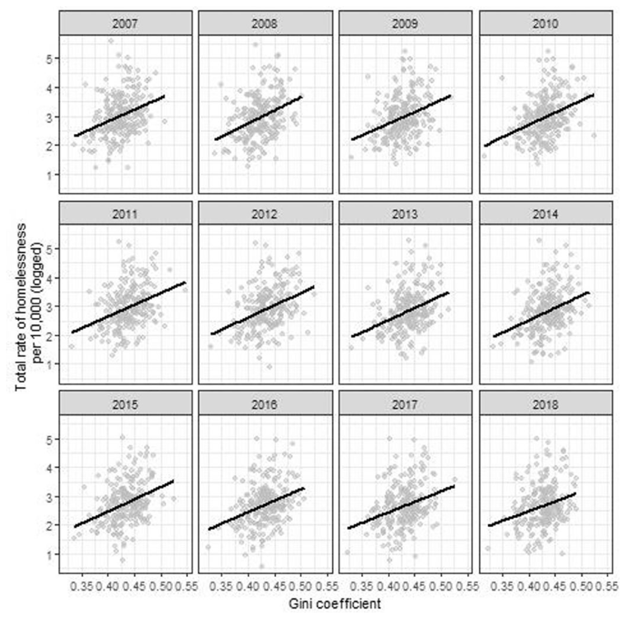
Between-Community Relationship of Income Inequality and Total Rate of Homelessness, 2007–2018
This evidence has led a few scholars to suggest income inequality as a potential structural driver of homelessness in the United States (Orlando 2013; Shinn 2010; O’Flaherty 1996), which is one of the world’s richest countries yet also one of the most unequal with higher rates of homelessness than its peer countries. Yet empirical research on whether and how income inequality impacts homelessness remains limited. We seek to address this gap with this study.
How Inequality Could Create Homelessness: A Theoretical Model
The rise of inequality in the United States has attracted significant attention in recent years, among academics and in politics, in part because incomes have grown faster for high-income households than for low- to middle-income (LMI) households since the late 1970s. As a result, high-income households now earn a larger share of the country’s annual output than they did only a few decades earlier.
Economists have tracked this evolution with several different measures. The classic Gini coefficient (Gini 1912), which we use in this analysis, has the benefit of being easy to approximate with only a rough breakdown of incomes across the distribution. The Gini coefficient estimates the degree to which the share of income earned by each percentile of the distribution differs from the share of the population in that percentile. It thus ranges from zero to one, with zero representing perfect equality (all households have the same income) and one representing perfect inequality (one household has all the income). 2 Figure 2 shows this measure alongside other measures of inequality, namely, the portion of national income earned by the richest 10 percent and 1 percent of the distribution, for comparison.
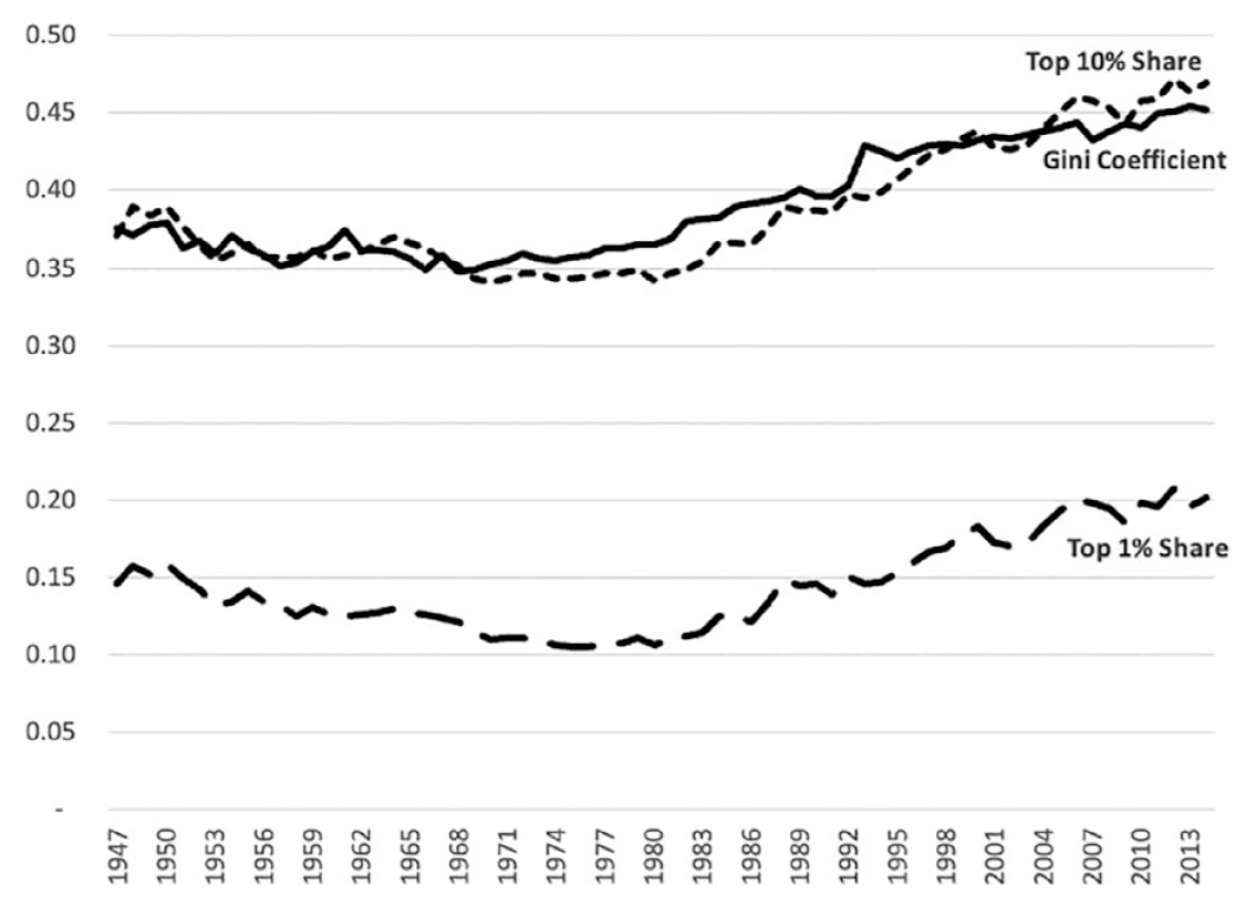
Comparison of Inequality Measures, 1947–2014
In all three cases, inequality declines slowly from 1950 to 1970. By 1980, all three measures are rising, and though there are a few cyclical pauses, they continue rising until the end of the time series. So sharp is this rise that the data pass their 1950 peak by 1990—and they keep rising thereafter. By 2014, the top 10 percent is earning nearly half of national income, and the top 1 percent has doubled its share, from one-tenth to two-tenths of every dollar produced. These measures likely understate the full extent of inequality, as they capture only annual income, not the full accumulation over time in the form of wealth. Access to saved funds, such as intergenerational transfers, is an important determinant of the ability to purchase a home, though they likely play a smaller role in monthly rent payments for low-income households. For these households living paycheck to paycheck, it is income that matters most—and moreover, it is in these income statistics that we find the most available data for our analysis.
Alongside this rise in inequality has been an equally troubling rise in housing costs, both for homeowners and for renters. This trend has accelerated since the end of the Great Recession, with housing prices and rents growing much faster than incomes, especially on the coasts, where major urban areas have restricted housing supply, making it unable to keep up with the influx of demand. In the wake of the financial and foreclosure crises, many borrowers found themselves shut out of the mortgage market, “diverting” these homeowners into the rental market (Myers et al. 2016). As a result, nearly half of renters are now “cost burdened,” meaning they spend at least 30 percent of their income on housing. In all, more than 37 million U.S. households are cost burdened, of which 18 million spend more than half of their income on housing (Joint Center for Housing Studies of Harvard University 2019). While this outcome may seem to be yet another effect of rising inequality, researchers have not established a convincing theoretical or empirical connection between the two. The similarities are too glaring to ignore. Just as the economy has grown rapidly for some and sluggishly for others, so too have the housing markets in many cities seen rapid price growth for homeowners at the same time as increasingly unbearable cost burdens for others, which may be key to understanding the uneven distribution of homelessness across the United States.
To understand this phenomenon, it is important to distinguish between two different types of inequality: between-city inequality and within-city inequality. As Diamond (2016), Ganong and Shoag (2017), and Hsieh and Moretti (2019) have shown, a significant contributor to the national rise in inequality has been the divergence between high-wage cities with high housing prices and high-skilled workers, on one hand, and low-wage cities with low housing prices and low-skilled workers, on the other hand. For a local phenomenon such as homelessness, it is inequality within each city, not between cities, that matters. That is, homelessness in Los Angeles is likely driven more by the dynamics of the housing market in Los Angeles than by the differences between Los Angeles and Kansas City. Thus, it is possible for homelessness to decline nationally and yet increase in Los Angeles if local inequality is increasing in Los Angeles but not in many other cities. (National inequality can still increase if between-city inequality is growing.) To better understand these dynamics, we consider how economic growth increases housing demand and propose two main mechanisms through which local inequality and local homelessness may be causally connected: what we call an “income channel” and a “price channel.”
The income channel
Let us begin with the theoretical construct that economic growth increases the demand for housing and thus the price of housing. If housing supply is inelastic, as a large body of evidence indicates it is for many U.S. cities (Saiz 2010; Glaeser and Gyourko 2018), new housing construction does not respond to this price increase, and not enough new housing (even of the higher-quality housing that will filter down to low-income households) is produced. The result is an increased housing cost burden for all households. If income growth is equally distributed, then housing cost burden is equally affected across the income distribution—that is, incomes rise proportionally across the income distribution to meet this increase in housing prices. Thus, the lowest-income households on the bottom tier of the housing ladder experience an income increase proportional to those at the top; if there is an increase in homelessness, it is because of the increase in prices, not because of differences in income growth. However, when income growth is skewed toward the highest-earning households, housing burden increases disproportionately for the bottom and middle of the income distribution. Thus, households toward the bottom of the income distribution will be relatively poorer than their fellow residents, who continue to drive up housing costs for the city as a whole. Even if the price growth is not abnormally high, low-income residents lose the competition to bidders with higher income growth. Some households will remain housed by devoting a larger share of their income toward housing, but others will be unable to afford housing at all, resulting in increased homelessness. This is what we refer to as the “income channel” through which inequality produces homelessness. For this channel to be true, we would expect income inequality to increase both homelessness and the share of low-income households who are rent burdened. 3
The price channel
Again, we return to the construct that economic growth increases the demand for housing and thus the price of such housing. However, cities with higher inequality attract faster housing price appreciation because they have more high-income, high-skilled, high-productivity workers, who increasingly command rents (i.e., have earnings that exceed their actual level of productivity) in the global economy. As a result, in the context of income inequality, low-income households will experience higher cost burdens not just because their income lags behind, but also because higher levels of income inequality will accelerate housing price growth. It is important to note that this cost acceleration can take the form not just of an increase in the purchase price of the houses but also of all the investments that go into the houses, including energy prices and renovation costs. This is the price channel mechanism by which increasing income inequality might increase homelessness. Even if income growth is equally distributed, these cities are so desirable that prices exceed the threshold of affordability for many low-income households.
Despite the highly plausible theoretical link between income inequality and homelessness, empirical evidence of such a relationship is somewhat limited. O’Flaherty (1996) presents some empirical support for his theory of the relationship between inequality and homelessness, although it is based on data from the 1970s and 1980s in only a handful of cities. Toro and colleagues (2007) and Shinn (2010) use cross-national comparisons between the United States and a number of European nations to show that countries with higher income inequality tend to have higher rates of homelessness. Finally, in the study most closely related to this one, Wood et al. (2015) use panel data from 328 localities in Australia to examine the structural drivers of homelessness, finding that within-community increases in the Gini coefficient are positively associated with the rate of homelessness.
Our study questions
The following study aims to understand whether rising income inequality increases homelessness at the local level. Further, if inequality does have an effect on homelessness, is it operating through the income channel, the price channel, or both? We leverage data on income inequality and homelessness from a large set of U.S. communities from 2007 to 2018. In doing so, our analysis offers the most robust analysis to date of how income inequality is related to homelessness in the United States.
Methods
Data
The current study relies primarily on publicly available data from HUD and the U.S. Census Bureau, which we use to construct a novel dataset that allows us to capture changes in income inequality, homelessness, renter cost burden, and home values in a sample of 239 communities over a 12-year period from 2007 to 2018. More precisely, these “communities” comprise single counties or aggregations of multiple counties known as Continuums of Care (CoCs), which are geographic units at which HUD administers federal homeless assistance dollars and at which local stakeholders conduct enumerations of the homeless population on an annual basis (see Mosley, this volume). To enable the construction of annual measures of income inequality, our sample includes the subset of CoCs that fully comprise counties above a certain population threshold (more than sixty-five thousand people). For the sake of simplicity, we use the terms community and CoC interchangeably throughout the remainder of the article. Below, we briefly describe the steps that we used to construct our dataset, with additional details provided in the online appendix.
First, to measure income inequality, we mirror the approach that Boustan and colleagues (2013) used. We aggregate data and microdata from the Census’ American Community Survey (ACS) to construct county-level Gini coefficients on an annual basis for each year from 2007 to 2018. We also obtain measures of renter cost burden, home values, and additional county-level variables from the ACS and other sources.
We then merge these county-level data with annual PIT counts of homelessness and annual data on the number of permanent supportive housing (PSH) units in a community from HUD. The inclusion of the number of PSH units in our analysis is important to account for recent expansions in PSH and the documented association between such expansions and reductions in homelessness (Evans et al. 2019).
We merge our county-level income inequality and other measures with the HUD data to construct a CoC-level dataset using a modified version of the process that Byrne and colleagues (2013) described. Because the ACS county-level measures that we use in our analysis are only available on an annual basis for counties with a population of sixty-five thousand or more, our final sample comprises 239 CoCs (out of 398 active CoCs in 2018) for which we have up to 12 years of data. These 239 communities account for 77 percent of the total number of persons experiencing homelessness nationwide on a given night in 2018. We conduct supplemental analysis using data from all CoCs for a limited number of years. Results from that analysis are similar to the main results and are detailed in the online appendix.
Analysis
Our analytic strategy involves estimating a series of regression models that explore the relationship between income inequality and total homelessness (measured as a rate per ten thousand members of the general population), the proportion of rent-burdened low-income renters (defined as households with income less than $20,000 paying more than 30 percent of income on rent), and median value of owner-occupied housing units (hereafter referred to as median home value) at the community level. The models using the latter two outcome measures allow us to test the “income channel” and “price channel” 4 mechanisms by which inequality might drive homelessness, respectively. In addition, to further explore the relationship between income inequality and homelessness, we estimate models in which we use homeless individuals, persons in families, sheltered homeless persons, unsheltered homeless persons, and chronically homeless persons as outcomes.
In all of these models, the Gini coefficient is the primary independent variable of interest, and we also control for the following set of time-varying control variables where appropriate: median household income, median rent for a two-bedroom apartment, median home value, poverty rate, real gross domestic product (GDP), and the number of PSH beds per ten thousand people. We briefly describe our modeling strategy here, with full details provided in the online appendix.
We estimate two types of regression models. First, we estimate a series of ordinary least squares (OLS) regression models. In addition to the time-varying control variables described above, these models also include community and year fixed effects. The inclusion of these fixed effects is intended to control for, respectively, any time-invariant differences between communities and any secular time trends that may confound the relationship between income inequality and homelessness.
Second, we use an instrumental variable (IV) approach to develop a more robust estimate of the causal impact of income inequality on our outcome. Specifically, a limitation of our OLS models is that they do not account for unobserved time-varying community-level characteristics that are possible confounders of the relationship between income inequality and our outcomes of interest and cannot rule out reverse causality. The IV approach helps to address these potential sources of bias and reverse causality by identifying a variable (the instrument) that isolates the portion of variation in our predictor (the Gini coefficient in this case) that is exogenously determined, thus allowing for a more robust assessment of its causal impact on the outcome of interest. In constructing our instrument, we follow the approach that Boustan and colleagues (2013) used. Briefly, this approach uses national changes in the income distribution as an instrument for variation in a community’s actual income distribution, with the assumption that national changes in income distribution are a source of exogenous variation in a community’s actual income distribution. We use this instrument to estimate the impact of income inequality on our outcomes using a two-stage least squares approach (2SLS). Our IV models also include community and year fixed effects.
Results
Table 1 presents summary statistics of the variables that we used in the analysis, averaged across the entire study period and in the first year (2007) and last year (2018) of the study period. The average Gini coefficient, pooled across all years and communities in the sample, was 0.438, and it increased, on average, within communities by about 0.004 (or just under 1 percent) over the entire study period. This relatively small average increase in the Gini coefficient over the study period masks a period of sharper increase over the early years of the study period and then a slight decrease over the later years. It also masks substantial heterogeneity across communities: roughly a third of communities experienced a one point or more increase in the Gini coefficient, and 18 percent experienced a decrease in the Gini coefficient of one point or more. Similarly, the total rate of homelessness decreased, on average, by 19 percent over the study period, but this masks substantial variation, with the rate of homelessness increasing, on average, in the latter years of the study period, and nearly 30 percent of communities in the sample experiencing an increase in the rate of homelessness between 2007 and 2018. It is this heterogeneity that allows us to identify the impact of income inequality on rates of homelessness.
Summary Statistics, 2007–2018

Tables 2 and 3 present the results of the OLS and IV models for the homelessness outcomes, respectively. The OLS estimates find that income inequality has a positive and significant relationship with the total rate of homelessness per ten thousand people, as well as with the rates of homelessness among individuals, people in families, and the rates of sheltered and chronic homelessness. The OLS model finds that a one-point increase in the Gini coefficient is associated with an increase in the total rate of homelessness of about 1.1 persons per 10,000 members of the general population. 5 In a community with a population of 740,000 (roughly the average population of communities in our sample, or equivalently, approximately the 2018 population of Seattle), this would translate into an increase of about eighty-one people experiencing homelessness. The coefficient estimates for the models using the rate of individual and family homelessness as outcomes suggest that this overall relationship appears to be driven more heavily by the relationship between income inequality and the rate of homelessness among individuals, as opposed to people in families. Similarly, the parameter estimate for the Gini coefficient in the model in which the rate of sheltered homelessness is the outcome suggests that the positive association between income inequality and the total rate of homelessness is driven largely by an increase in the rate of sheltered homelessness. The relatively weaker relationship between income inequality and chronic homelessness makes sense, as we would expect chronic homelessness to be less sensitive to the income and price channel mechanisms that we consider as drivers of the relationship between inequality and homelessness.
Ordinary Least Squares (OLS) Models of the Relationship between Income Inequality and Homelessness

NOTE: All models include CoC and year fixed effects. Robust standard errors clustered at CoC level shown in parentheses.
p < .05. **p < .01. ***p < .001.
Instrumental Variable (IV) Models of the Relationship between Income Inequality and Homelessness

NOTE: All models include CoC and year fixed effects. Robust standard errors clustered at CoC level shown in parentheses.
p < .05. **p < .01. ***p < .001.
The IV estimates shown in Table 3 represent our preferred specification and are consistent with the OLS estimates: the parameter estimates for our Gini coefficient measure are positive and significant in the models for the total rate of homelessness, the rates of homelessness among individuals and persons and families, and the rates of sheltered and chronic homelessness. Moreover, as with the OLS models, the parameter estimates for the Gini coefficient are relatively stronger in both the models for individuals and for sheltered homelessness. However, the magnitude of the coefficients in the IV models are substantially larger than in the OLS models. For example, in the model for the total rate of homelessness, the IV estimates indicate that a one-point increase in the Gini coefficient generates an increase in the total rate of homelessness of 7.6 persons per 10,000 members of the general population. Returning to our example of a hypothetical community with a population of 740,000, this means that a one-point increase in the Gini coefficient would result in an increase of about 562 people experiencing homelessness on a given night. Another way of contextualizing this estimate is by applying the average change in the Gini coefficient observed across all communities in our sample over the study period, which was an increase of 0.37 points. In a community with a population of 740,000, this would translate into an additional 208 people experiencing homelessness on a given night. 6
To examine whether our price channel and income channel mechanisms might be driving the relationship between income inequality and homelessness, Table 4 presents the results of the models in which we use the proportion of rent-burdened low-income renters and median home values as our outcomes. For the proportion of rent-burdened renters, the OLS model finds a positive, but not statistically significant, relationship between income inequality and the share of rent-burdened low-income renters. However, the IV model finds a positive and significant effect of income inequality on the proportion of rent-burdened low-income renters, with a one-point increase in the Gini coefficient leading to a 0.86 percentage point increase in the proportion of rent-burdened low-income renters. For the median home value models, the OLS specifications find a significant negative association between the Gini coefficient and home values, while the IV estimates do not find a significant association between the Gini coefficient and home values. Thus, in examining the mechanism by which income inequality generates homelessness, we find more support for the income channel than for the price channel.
Models of the Relationships between Income Inequality, Proportion Rent Burdened Low-Income Renters and Home Values

NOTE: All models include CoC and year fixed effects. Robust standard errors clustered at CoC level shown in parentheses.
p < .05. **p < .01. ***p < .001.
Discussion
We return to our original questions of whether local income inequality generates homelessness and, if so, what is the mechanism through which it does. Our results are clear in showing a link between local income inequality and homelessness, and our IV estimates suggest that this relationship is causal in nature. Notably, our findings suggest that the impact of income inequality on homelessness is driven by changes in sheltered, but not unsheltered, homelessness. That we did not find evidence of a link between inequality and unsheltered homelessness could be due to measurement error, as there are long-standing methodological challenges in enumerating the unsheltered population, the degree of which varies across communities (Glynn and Fox 2019). Alternatively, because the rate of sheltered homelessness depends on shelter capacity, our findings may also suggest that income inequality is linked to whether a community responds to homelessness through an expansion of emergency shelter.
Our findings that income inequality has a positive impact on renter cost burden but not home values also suggest that the income channel is the more likely causal mechanism through which income inequality impacts homelessness. Because our findings are not sufficiently robust to fully untangle the relationships between income inequality, renter cost burden, home values, and homelessness, we offer only tentative evidence in favor of the income channel. Consequently, we hope our findings offer a point of departure for future research to fully explore these mechanisms.
Of course, our investigation of the impact of income inequality on homelessness is not just an academic exercise. Our findings have implications for policy and programmatic efforts to address homelessness. We envision such efforts operating at three different levels.
First, our results suggest that broader policy efforts to reduce income inequality would have the collateral benefit of reducing homelessness. Thus, our study provides yet another brick in the wall of the argument that we should pursue aggressive policy responses to reverse decades-long trends in income inequality in the United States.
Second, our results suggest that policy and programmatic efforts intended specifically to address homelessness are needed more sorely in places where income inequality has been increasing more quickly. Our tentative evidence in favor of the income channel points to specific types of policy responses that may be warranted. In particular, while many housing policy advocates focus on slowing the growth of housing prices, this strategy alone is unlikely to be sufficient in preventing homelessness. It is important to include policies that increase the ability of low-income households to afford housing—for example, increasing the minimum wage, public benefit levels, and the supply of Section 8 Housing Choice Vouchers. Because this problem is so specific to these high-inequality localities, it especially makes sense for these localities to adopt their own solutions rather than a one-size-fits-all federal policy. For example, Los Angeles has effectively created its own Section 8 program through its Department of Public Health for people experiencing homelessness and is currently providing prepaid debit cards as a direct cash subsidy to low-income families who have been affected by the COVID-19 pandemic.
Finally, these findings point to the importance of local, as distinct from national, inequality. While most of the research literature and the public debate have focused on the macro level of analysis, this study reveals that the city level is what matters for homelessness. It is the ability of high-income residents to outcompete low-income residents that leads to the exclusion of the latter group from the housing market. The significance of the income channel, rather than the price channel, confirms this finding. Homelessness is less associated with the divergence between high-priced and low-priced cities than it is with the divergence between residents of the same city. Hopefully, this conclusion inspires future research to explore why some cities have higher levels and growth rates of inequality and what targeted policies can reverse these local trajectories, rather than relying on federal policies that are poorly attuned to the needs of different local housing markets. If policy-makers focus only on slowing the growth of prices in cities like New York and Los Angeles, it is likely to be insufficient to solve the homelessness crisis. They must also consider the ways in which some neighborhoods are given more access to opportunity than others, whether through segregation or locally financed education or the spatial mismatch of jobs and housing. Homelessness is more than a problem of dollars and cents. It is a symptom of a deeper challenge, fundamental to the very structure of our society: how do we share this Earth with our fellow human beings, with all that each location has to offer and all that each person deserves to experience?
Supplemental Material
sj-docx-1-ann-10.1177_0002716220981864 – Supplemental material for A Rising Tide Drowns Unstable Boats: How Inequality Creates Homelessness
Supplemental material, sj-docx-1-ann-10.1177_0002716220981864 for A Rising Tide Drowns Unstable Boats: How Inequality Creates Homelessness by Barrett A. Lee, Marybeth Shinn, Dennis P. Culhane, Thomas H. Byrne, Benjamin F. Henwood and Anthony W. Orlando in The ANNALS of the American Academy of Political and Social Science
Footnotes
Note:
The authors wish to acknowledge Leah Boustan for providing the data and code that were essential in constructing the measures of income inequality that we used in this study.
Notes
Thomas H. Byrne is an assistant professor at the Boston University School of Social Work and an investigator at the U.S. Department of Veterans Affairs Center for Healthcare Outcomes and Implementation Research and National Center on Homelessness among Veterans.
Benjamin F. Henwood is an associate professor and the director of the Center for Homelessness, Housing and Health Equity Research at the University of Southern California Suzanne Dworak-Peck School of Social Work. He is a lead author in the American Academy of Social Work and Social Welfare’s The Grand Challenge of Ending Homelessness.
Anthony W. Orlando is an assistant professor of finance, real estate, & law and Donor’s Scholar of Analytics at California State Polytechnic University, Pomona. He is a visiting scholar at the Federal Reserve Bank of Atlanta and faculty affiliate of the USC Bedrosian Center on Governance and the Public Enterprise.
References
Supplementary Material
Please find the following supplemental material available below.
For Open Access articles published under a Creative Commons License, all supplemental material carries the same license as the article it is associated with.
For non-Open Access articles published, all supplemental material carries a non-exclusive license, and permission requests for re-use of supplemental material or any part of supplemental material shall be sent directly to the copyright owner as specified in the copyright notice associated with the article.
