



Abstract
Standard measures of residential segregation tend to equate spatial with social proximity. This assumption has been increasingly subject to critique among demographers and ethnographers and becomes especially problematic in historical settings. In the late nineteenth-century United States, standard measures suggest a counterintuitive pattern: southern cities, with their long history of racial inequality, had less residential segregation than urban areas considered to be more racially tolerant. By using census enumeration procedures, we develop a sequence measure that captures a more subtle “backyard” pattern of segregation, where white families dominated front streets and blacks were relegated to alleys. Our analysis of complete household data from the 1880 Census documents how segregation took various forms across the postbellum United States. Whereas northern cities developed segregation via racialized neighborhoods, substituting residential inequality for the status inequality of slavery, southern cities embraced street-front segregation that reproduced the racial inequality that existed under slavery.
Starting from human ecology models of urban racial patterns, studies of residential segregation tend to assume that individuals have a higher probability of social contact with people who live geographically close rather than those who live further away. Most quantitative measures of segregation, including aspatial (Massey and Denton 1988) and spatial (Reardon and O’Sullivan 2004; Reardon et al. 2008) indices, are based on a premise that equates proximity with potential interaction between individuals from different racial groups. This assumption, however, is increasingly subject to critique by ethnographers and demographers, who contend that spatial distance does not adequately capture the lived experience of segregation. Urban ethnographers trace segregation through walking tours that document racial interaction in public spaces and along pedestrian paths, albeit ones that often do not follow the dictates of spatial proximity (Anderson 1992, 2011; Duneier 1994, 2013; Molotch 1972). Likewise, demographers suggest that modern urban populations tend to interact with others who live “down the street” from them (Grannis 1998, 2009), while recognizing that straight-line distance remains an influential predictor of sociability (Hipp and Perrin 2009). These critiques imply that the residential patterning of racial groups may be better explained by models based on street networks and other features of neighborhoods rather than models based exclusively on geographic propinquity or administrative boundaries among census tracts.
The use of spatial distance as equivalent to social distance becomes especially problematic in the historical study of residential segregation. Quantitative measures of residential segregation in the United States point to a counterintuitive pattern, in which urban areas with a history of extreme racial inequality have lower segregation scores than urban areas that are considered to be more racially tolerant. This pattern can be traced back to the nineteenth century, when blacks who were engaged as slaves or servants lived in close proximity to the whites who owned or employed them (Lieberson 1963; Massey and Denton 1993; Taeuber and Taeuber 1965). In the 1960s and 1970s, a thriving demographic literature demonstrated that southern cities that represented the oldest urban centers of the region—and thus had the deepest roots in slavery—also historically ranked lower on standard indices of segregation, such as the index of dissimilarity (Roof, Valey, and Spain 1976; Schnore and Evenson 1966). At the same time, qualitative evidence for some southern cities suggests these rankings did not signal racial integration, but might be associated with a more subtle “backyard” pattern of segregation, where white families dominated front streets and blacks were relegated to living on smaller streets and alleys (Demerath and Gilmore 1954; Johnson [1943] 1970; Spain 1979). Rooted in a legacy of slavery and indicative of highly unequal status relationships between blacks and whites, the pattern of segregation along street networks was not captured by conventional measures of segregation.
This article advances scholarship on racial residential segregation by theorizing and empirically examining how the structural bases of the “backyard” pattern vary from other dimensions of segregation. We build on the early work of Agresti (1980) to develop a sequence measure that documents street-front segregation. The measure offers several advantages over existing measures, especially in regard to the historical study of residential segregation. By using census enumeration procedures, it incorporates detailed spatial relations between housing units without recourse to household addresses or historical maps of urban centers. Moreover, it offers an approach that differentiates the backyard pattern from other forms of segregation, based on either straight-line spatial distance or boundaries between wards, districts, or census tracts. To investigate the empirical properties of the measure, we focus on a single city, Washington, DC, where surviving census district maps combined with the 1880 Census allow us to geocode households and draw detailed comparisons with other spatial and aspatial measures of residential segregation.
We then move to a broader analysis of residential segregation in the postbellum United States, comparing the sequence measure with the index of dissimilarity in 171 cities and towns. Our analysis points to three findings that advance the literature on segregation. First, whereas previous evidence was qualitative and limited to a few southern cities, we empirically quantify the extent of the backyard pattern across all U.S. urban centers in the late nineteenth century. Second, we find that segregation took different forms across the postbellum United States. Confirming the intuitions of historical case studies, the U.S. South was indeed more susceptible to street-front segregation (or segregation via other neighborhood features) before the widespread diffusion of Jim Crow laws, whereas the Northeast was more susceptible to the emergence of segregated African American districts. This regional divergence highlights the importance of distinguishing the micro-level impact of racial segregation on pedestrian patterns from its macro-level impact on the spatial separation of households.
Third, we show that the theoretical explanation of residential segregation varies by its form. Street-front segregation reproduced the residential inequality that had once existed under slavery. As a result, this form of segregation was more likely to be observed in cities where blacks represented a larger proportion of the urban population and where blacks worked in occupations that brought them into regular contact with white employers, such as domestic service. By contrast, the formation of racialized districts substituted residential inequality for the status inequality of slavery. Blacks were more likely to be segregated via racialized neighborhoods in younger cities, cities where more time had passed since the abolition of slavery, and cities where blacks represented a smaller share of the population. In the late nineteenth century, these features accounted for much of the regional divergence between the cities of the South and the Northeast, offering a structural explanation for historical differences in the origins and forms of U.S. racial segregation.
Dimensions of Historical Segregation
Past research on historical residential segregation largely uses aspatial measures, mostly based on the index of dissimilarity (e.g., Berlin [1974] 2007; Cutler, Glaeser, and Vigdor 1999; Lieberson 1963; Taeuber and Taeuber 1965; Trotter 1985; Tuckel, Schlichting, and Maisel 2007), but also the isolation index (Cutler et al. 1999; Gotham 2000; Lieberson 1980; Massey and Denton 1993) and the Gini index (Rhode and Strumpf 2003). Although aspatial indices of segregation have been repeatedly criticized on methodological grounds (see Reardon and O’Sullivan 2004), the use of spatial measures of segregation in historical research continues to be limited by data availability. Calculation of spatial indices of segregation requires geographic data (e.g., addresses or maps of census divisions, such as enumeration districts or blocks) that are only available for some cities in historical studies (e.g., Spielman and Logan 2013). Aspatial segregation measures tend to rely on relatively coarse geographic boundaries, such as city wards, when deployed in historical settings.
More importantly, neither spatial nor aspatial indices capture patterns of residential segregation along streets or walking networks, where pedestrian paths are most likely to lead to face-to-face encounters between individuals from different social groups. Grannis (1998, 2009) suggests that small residential streets are the basis of neighborly interactions in modern urban centers. Examining communities formed by tertiary street networks in Chicago, Los Angeles, and New York, he finds they are a potent source of racial homogeneity, after controlling for spatial distance between block groups (Grannis 2005). 1 Arguably, small streets and other neighborhood features are even more important to residential interaction when viewed historically, owing to the greater prevalence of foot and other non-vehicular traffic (Massey and Denton 1993). Writing in the early 1940s, Johnson ([1943] 1970:9) found a number of isolated black communities in the U.S. South resulting from pedestrian boundaries “marked by a railroad track, stream, or other fixed barrier” (see also Ananat 2011). In other urban clusters, he suggested that “the location of many Negro homes near places of employment (as domestics) [had] established a large degree of tolerance [among whites] of Negro neighbors” (Johnson [1943] 1970:10). Even in such locales, other forms of segregation and social distance tended to substitute for physical separation between blacks and whites.
The backyard pattern was the classic form of segregation in the postbellum South. Johnson associated this pattern with Charleston, South Carolina, in particular, where clusters of residences for black servants or tenants could often be found in the rear of affluent white families’ homes. Subsequently, social historians identified variants of the pattern in other urban centers across the South (Demerath and Gilmore 1954; Myrdal 1944; Taeuber and Taeuber 1965). In antebellum New Orleans, for instance, conditions of servitude and limited land availability led to widespread intermingling of slave and free black residences with white households (Spain 1979). However, the physical organization of households preserved social distance between blacks and whites. Homes of wealthy (and often slave-owning) whites faced wide boulevards on the exterior of “superblocks,” while blacks lived on small interior streets and alleyways. This pattern initially persisted during the postbellum period, although the spatial segregation of blacks in New Orleans subsequently increased, precipitated by the introduction of Jim Crow and the expansion of the city’s streetcar system after 1900 (Spain 1979).
In the emerging cities of the New South, black urban clusters tended to be small and scattered in the late nineteenth century. Cities such as Lexington, Kentucky, Durham, North Carolina, and Atlanta, Georgia, did not exhibit the backyard pattern of segregation. Nevertheless, black districts formed in narrow zones characterized by undesirable living conditions or depressed land prices. In lieu of tertiary streets, these zones were defined by other features of local topography or land use, such as railroad tracks, cemeteries, city dumps, factories, and land with steep slopes or poor drainage (Kellogg 1977). Although white households were often not distant from black districts, they were more likely to be located on higher ground and away from public nuisances. Topography and land prices sustained the social separation of blacks and whites even though the black population was fairly dispersed in many cities of the New South.
These considerations point to a pattern of residential segregation distinct from the dimensions usually assessed by aspatial and spatial measures of segregation (see Figure 1). Traditional aspatial indices capture the separation of social groups across administratively or politically defined geographic boundaries. This separation—which we call primary (or p-) segregation—offers only a crude assessment of the capacity of members of different groups to interact, particularly when physical segregation tends to be more local than the boundaries used in administrative data. As an alternative, much of the recent methodological literature points to spatial indices as a means to capture the separation of social groups, even if they happen to be located within the boundaries of the same administrative units. In this conception, segregation occurs through the separation of groups along straight-line paths in physical space. Assessment of this separation—which we call secondary (or s-) segregation—offers important methodological advances, in terms of addressing the modifiable areal unit problem (MAUP) and taking full advantage of the geographic information available from recent censuses (Reardon and O’Sullivan 2004). 2 It does not, however, address the concern that segregation may largely be a function of residential street layout or other neighborhood features that influence pedestrian paths (Grannis 2009).

Dimensions of Residential Segregation
We call this third dimension of separation between groups tertiary (or t-) segregation. As suggested by historical examples, such as the backyard pattern and black urban clusters in the South, social groups can be separated through tertiary segregation while living in reasonably close spatial proximity or residing in the same wards or census districts. Myrdal (1944:621) famously described the backyard pattern as one where “Negroes usually live in side streets or along alleys [in] back of the residences of whites.” Johnson ([1943] 1970:9–11) noted similarly that several forms of residential segregation feature some “accommodation to racial proximity,” including the backyard pattern itself, dispersed clusters of blacks in southern cities, and street-side segregation (“in which white people are found occupying one side of the street and Negroes the other”). A common feature of these residential arrangements is that the straight-line distance between white and black households is low. Yet pedestrian pathways that differentiate front streets from alleys—or that are constrained by the separation of households across busy streets or other physical barriers—preserve the micro-segregation experienced by residents.
Structural Bases of Segregation
Modern and historical treatments of racial segregation suggest that tertiary segregation may not only be conceptually distinct from primary and secondary segregation, it may be explained by different mechanisms as well. If so, theorizing the structural foundations of tertiary segregation—and how they diverge from other dimensions of segregation—remains a central task of historical demography.
The distribution of employment opportunities exercised a strong historical constraint on the location of black households. Emerging in a time when slaves were compelled to attend to the needs of white households, the backyard pattern often persisted where blacks lived near white employers, but whites sought to preserve status boundaries through the physical arrangement of residences (Johnson [1943] 1970; Wilson 2012). Cities with substantial numbers of black domestic servants in the postbellum period were especially susceptible to street-front segregation. Urban patterns of residential organization were also affected by small-scale manufacturing (Massey and Denton 1993). In cities that depended on blacks to work in workshops, tanyards, mills, and other small manufactories, black households were clustered in the alleyways around these enterprises (Kellogg 1977). White households were often located nearby, but they tended to be up the hill or across the tracks, away from industrial nuisances. T-segregation thus minimized the spatial mismatch found in some modern U.S. cities, where blacks are both physically and socially isolated from labor market opportunities due to their places of residence (Ovadia 2003). 3
The prevalence of the black population in cities is another factor associated with historical levels of residential segregation. In recent decades, black minority representation sometimes increases the level of black-white segregation, with common explanations rooted in minority threat theories (in which whites are more likely to exclude blacks when they experience psychological threat from a larger black population) or ecological theories (in which black enclaves become more self-sufficient as the black population expands) (Blalock 1967; Iceland, Sharp, and Timberlake 2013; Logan, Stults, and Farley 2004; Marshall and Jiobu 1975). Historically, the creation of spatially isolated enclaves of blacks was far more politically fraught in many U.S. cities. Among whites, there was a widespread distrust of a cohesive black community and a desire to monitor blacks intensively (Spain 1979). This was particularly true in the U.S. South, where 17 cities (including Atlanta, Charleston, Houston, and Savannah) had majority or near-majority (over 40 percent) black populations in 1880.
In urban areas, several mechanisms linked black population size with the preservation or emergence of tertiary segregation. One mechanism was that the legacy of slavery left small, poorly built dwellings that were originally intended for slaves in the back of, around the corner, or across the street from better residences owned by whites. Occupying former slave quarters carried a considerable amount of stigma in the postbellum period, but the limited housing supply made it a necessity for blacks in many southern cities. Given crowding, high rents, and discriminatory restrictions on housing choice (Myrdal 1944), blacks were especially likely to move into these housing units when a city had a large or increasing black population.
A related mechanism accounting for tertiary segregation was the effort to manage interracial contact. The avoidance of direct physical contact between blacks and whites was a central driver in patterns of segregation (Johnson [1943] 1970). In cities with large black populations, spatial proximity between black and white households made interracial contact far more likely. In these contexts, Myrdal (1944:621) observed that segregation was based on what he identified as “‘ceremonial’ distance rather than spatial distance.” Ceremonial distance was maintained insofar as black residences were located out of public view, on backstreets and alleys in mixed-race neighborhoods. Within this residential pattern, socializing among white neighbors and play activities among white children were thought to be the province of front streets and more visible recreational areas, while socializing among black neighbors and play activities among black children were thought to be the province of back streets and alleys. From the perspective of white residents, t-segregation managed perceptions of minority threat and maintained social distance in urban locales where the black population was ubiquitous.
The pioneering work of Schnore and Evenson (1966) identified city age as another historical predictor of segregation. Older cities, particularly in the South, with a longer legacy of slavery were especially likely to maintain spatial proximity between black and white households. As Woodward ([1955] 2002:14–15) argued, a “pattern of residential intermixture prevailed to the end of slavery—and did not disappear quickly thereafter.” It was only gradually that “the new order added physical distance to the social distance between the races” (Woodward [1955] 2002:22; see also Roof et al. 1976). On this basis, we expect primary and secondary segregation decreased substantially with city age and increased with the time lag since emancipation. 4
On the whole, these mechanisms suggest a divergence between the structural bases for primary or secondary segregation, on the one hand, and tertiary segregation, on the other. Historically, the former dimensions substituted residential inequality for the status inequality of slavery. In the late nineteenth-century United States, the isolation of blacks in separate neighborhoods could be expected in newer cities, cities where more time had elapsed since emancipation, and cities where blacks remained a minority of the population. T-segregation, on the other hand, reproduced the residential inequality that had once been found under slavery. Street-front segregation was most likely in cities where blacks’ occupations brought them into regular contact with white employers and where blacks represented a larger proportion of the urban population. This residential pattern was unlikely to decay with the passage of time following emancipation.
The Sequence Index of Segregation
Our methodological approach builds on previous attempts to use census enumeration procedures to construct measures of segregation applicable in historical contexts (Agresti 1980; White, Dymowski, and Wang 1994). Drawing on Agresti (1980), we propose a Sequence Index of Segregation (SIS) that uses the ordering of households in census population listings as the basis for a measure of tertiary residential segregation. Historical population schedules consist of listings of every resident in every household visited by census enumerators, along with other information collected as part of the census. The SIS measure rests on the assumptions (examined further below) that households adjacent in census listings were neighboring and that enumerators followed typical pedestrian pathways due to census enumeration procedures. We test whether racial sequences in the population listings are serially independent—that is, we compare the observed degree of interspersal between two categories (whites and blacks in our analysis) to what would be expected under a random order. We compute the index of segregation by dividing the observed number of racially alike “runs” of households R by the expected number E(R) and subtracting this ratio from one:

where a run is a continuous sequence of individuals of the same race in a longer sequence of individuals from two racial groups. 5 Following Agresti (1980) and Wald and Wolfowitz (1940), the expected number of runs E(R) is calculated as

with N1 and N2 representing the number of individuals from the two racial groups that are observed in the entire sequence.
The SIS measure compares the actual amount of segregation along the path of an enumerator to that which would be observed under conditions of randomness. A value of one indicates complete segregation of the racial groups, with only two runs. A value of zero indicates random integration, when the observed number of runs in a sequence is equal to the expected number of runs. It is also possible for the SIS to be negative, when random interspersal would give rise to fewer runs than the actual sequence of residence among two racial groups, potentially as a result of conscious urban planning. Following Agresti (1980), the theoretical maximum for the number of runs in a sequence is equal to

A statistical property of the SIS, especially favorable in historical contexts, is that it can be applied to very small settlements or areas with a very small minority population. In particular, the distribution of the number of runs is approximately normal as long as the number of white households and number of black households are both greater than 10 (Brunk 1975). Recent simulation studies suggest that sequence measures can clearly differentiate between instances of complete segregation and no segregation as long as minority populations have more than five households in an area (Logan and Parman 2014).
Although the sequence-based measure of segregation using the logic of runs was first proposed by Agresti more than 30 years ago, it has received very limited application, primarily for data and methodological reasons. Until recently, use of historical micro-census data tended to involve tedious primary data collection. Historical demographers had to go into archives for particular towns and regions and analyze long hand-written listings of census enumerations. Now these microdata are increasingly available in electronic form (e.g., via the Integrated Public Use Microdata Series) (Ruggles 2014). Another data limitation acknowledged by Agresti (1980) was the limited time coverage for micro-census releases. At the time, the U.S. Census had not released enumeration forms for years beyond 1900 (because individual records are sealed for 72 years due to confidentiality considerations). Additionally, virtually all of the 1890 records were destroyed in a fire. Consequently, researchers had to rely on a very short time series. Now the same data are available until 1940 (with identifying information) and the present (without).
Most importantly, the methodological properties of the SIS as a measure of tertiary segregation were left unexamined. The assumption of ordered population listings was not analyzed empirically; the measure was not compared with alternative indices of segregation; and, finally, the measure’s reliability was assumed rather than tested. Without a careful examination of the empirical properties of the SIS, its utility for segregation research remains uncertain. Therefore, our primary methodological improvement on Agresti involves analysis of the SIS’s validity and reliability, to which we turn next.
Analysis of Racial Segregation in Washington, DC
To evaluate the accuracy and consistency of the SIS measure, we focus on Washington, DC, in 1880. The choice of the year and the city was driven by substantive and data considerations. The 1880 Census was the last population schedule collected before the widespread diffusion of Jim Crow laws and before the Civil Rights Act of 1875 (which sought to prevent racially biased access to public transportation and amenities) was declared unconstitutional in 1883. The census provides an informative baseline of the levels of racial segregation that resulted in the aftermath of slavery. Washington, DC, serves as a strategic research site for studying segregation, because it was a border city during the antebellum era, with a relatively large free black population and a mixture of prototypical northern and southern patterns of racial residence. 6 Data considerations also point to the utility of studying the pattern of residential segregation in Washington at the time. Among all nineteenth-century censuses, the 1880 Census is the only one for which geocoded data for the entire population (i.e., 100 percent enumeration) are currently available via IPUMS (Ruggles et al. 2010). 7 Washington is one of the few cities in the 1880 IPUMS data file for which the complete street address data required for spatial analysis have been released.
In 1880, the population of Washington, DC, included 149,057 inhabitants. We exclude the institutionalized population, non-whites and non-blacks, and cases that fall in the category of “partner, friend, or visitor” (based on their relationship to the household head). The resulting sample size is 143,251 and consists of 29,145 households. Because mixed-race households (apart from servants) were quite rare in 1880 (less than .1 percent of the total), we limit our analysis to the race of household heads, treating households themselves as racially homogeneous. 8 Our final sample includes white (67 percent) and black (33 percent) household heads with a total of 29,145 cases.
From 1880 until 1930, records in the census were arranged by enumeration districts. In the 1880 Census, the city of Washington, DC, was divided into 82 enumeration districts, numbered from 9 to 90 (the first eight districts were in the suburbs). The number of households per district ranged between 108 and 710, with a mean of 421 and standard deviation of 149. Our analysis includes only residents living within the city limits. Because enumeration districts were the smallest geographic unit above the address level in the 1880 Census, we use these districts for purposes of aspatial analysis and detailed comparisons across segregation measures.
Use of enumeration districts as units of analysis offers several theoretical advantages. First, the districts were defined so that most enumerators were residents and would be intimately familiar with these areas and their inhabitants. The “high degree of local knowledge” on the part of enumerators (Ruggles and Menard 1994:161) suggests their paths resembled those of other neighborly interactions. Second, enumeration districts provided clear boundaries for enumerators, often on the basis of civil divisions, with an eye toward allowing enumerators to travel the districts on foot within a relatively short time period. As a result, the districts represent geographic areas where residents could feasibly know any of their neighbors, and interact with them on a regular basis, but might be constrained from doing so by the layout of street networks, physical barriers, and social divisions.
For the spatial analyses, we used several maps. We examined the 1880 Census enumeration district map (National Archives and Records Administration 2003) and supplemented it with an antebellum landownership map (McClelland, Blanchard, and Mohun 1861), reflecting building sites and patterns of land use immediately before the end of slavery in the District of Columbia. Because both maps are image-based, we then georeferenced them in ArcGIS 10.2 (Environmental Systems Research Institute 2013) using the modern map of Washington streets (District Department of Transportation 2012) as a control layer. The control layer is informative because the city’s street layout has changed very little since the 1880s. We also used the 1888 Sanborn map for Washington (Sanborn Map Company 2001) to locate streets that had been renamed since the late nineteenth century or do not exist anymore.
Construct Validity of SIS
The basis for the sequence-based index of segregation rests on the assumption that most households listed consecutively in the census population listings were also neighbors in real life (Agresti 1980). Starting with the 1850 Census, the instructions to enumerators explicitly required them to number households “in the order of visitation” and to maintain records in the same order (U.S. Census Bureau 2002:19; Wright and Hunt 1900). Furthermore, because enumerators had to visit every household, census takers moved in a systematic sequence between neighboring households along well-established pedestrian routes. Historical evidence on census procedures suggests that enumerators indeed “went from cabin to cabin” (Magnuson and King 1995) or house-to-house down the same street, across the street, or around the corner. Enumeration instructions asked enumerators to leave blanks for households that were occupied but had no respondent present. Enumeration sequences were often preserved by filling in those blanks in subsequent visits (Logan and Parman 2014).
To examine whether the assumption of sequential street-front enumeration is valid, we geocoded the census data and traced the local enumerator’s visitation route. 9 We illustrate our analysis using enumeration district 10, located in the Georgetown area of Washington, DC (see Figure 2). 10 When sorted by the order of visitation, the census listings reveal continuous street sequences (see Table 1). For instance, 59 observations with serial numbers 884457 to 884515, and four observations with serial numbers 884523 to 884526, were located on High Street (now Wisconsin Avenue). For one house on High Street, the enumerator had to return, presumably because its residents were absent during the initial enumeration. However, such interruptions in street sequences are rare, representing less than 5 percent of the total street sequences in Washington. Because the serial number represents the order in which households were enumerated, we can infer that the enumerator first completed the boundary streets and then visited households on the interior of the city block. The pattern of visitation is consistent with our conceptualization of t-segregation, which considers the adjacency of households on the front streets of city blocks separately from their adjacency to households on streets and alleys within a block.

1880 Census Population Map for Enumeration District 10 in Washington, DC
Ordered Sequences of Serial Numbers and Enumeration Route for Enumeration District 10

Note: N = 253 cases.
Discriminant Validity of SIS
We next compared the SIS with other measures of segregation for Washington, DC. Because the SIS assesses segregation at a small scale and with attention to various constraints on social interaction (including the layout of street networks), its values are consistently higher than those of other commonly used measures of segregation, both spatial and aspatial (see Table 2). 11 Although the corresponding aspatial and spatial measures (e.g., the aspatial and spatial dissimilarity index) have almost identical values, the higher value of the SIS suggests it captures barriers between white and black households that are not reflected in other dimensions of residential segregation.
City-Level Indices of Segregation between Blacks and Whites, Washington, DC, 1880

Source: Authors’ calculations using the 1880 Census data.
To examine the discriminant validity of the SIS at a more fine-grained level, we contrasted the SIS values with the spatial dissimilarity index (
Comparison of SIS with
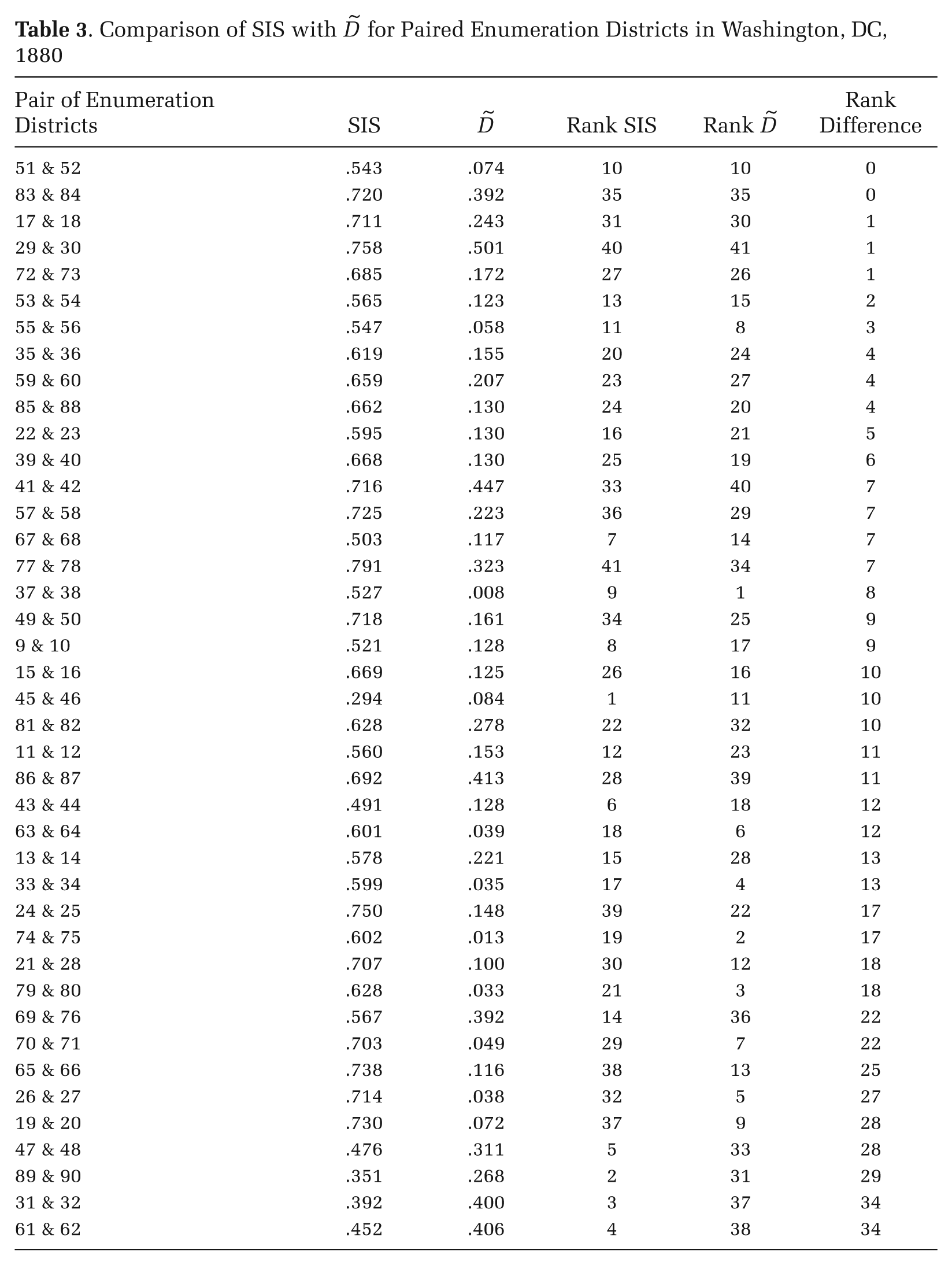
The SIS and spatial
Reliability of SIS
Because the SIS is based on the order of enumeration, one concern that may arise is how sensitive it is to variation in enumeration route, for example, to the sequence of streets chosen by a census taker. We conducted a simulation analysis of SIS reliability within an enumeration district, again focusing on District 10. Each district street represents a potential starting point for enumeration. If enumerators followed a rule of spatial contiguity, then the enumeration of a street could be followed by any adjoining street that had not already been canvassed. If enumerators followed a rule of random routing, then the enumeration could be followed by any remaining street in the district that had not already been canvassed. Additionally, boundary streets could be enumerated in either direction, and internal streets could be enumerated in either direction and through side-by-side enumeration of households (on the same side of the street) or alternating sides (by crossing the street after enumerating each household). 15
Our simulation analysis of SIS reliability thus considers four possible routing scenarios with respect to street sequencing and the enumeration of internal streets: (1) random routing, internal streets enumerated side-by-side; (2) random routing, internal streets enumerated side-by-side or by alternating sides; (3) streets ordered based on spatial contiguity, internal streets enumerated side-by-side; and (4) streets ordered based on spatial contiguity, internal streets enumerated side-by-side or by alternating sides. For each scenario, we computed SIS values for 1,000 simulated sequences within District 10. Under all possible routing scenarios, the SIS takes a limited number of values, all of which are close to or include the observed value of .544 (see Table 4). These simulation results suggest the SIS exhibits little sensitivity to different starting and ending points, route variation, or different direction of enumeration along streets.
Distribution of SIS Values Assuming Different Enumeration Scenarios, Enumeration District 10 (percentages)

Note: N = 1,000 sequences.
Calculating the SIS across enumeration districts, aggregation could also introduce noise into the measure, similar to the modifiable areal unit problem for aspatial indices. When the SIS is computed at the city-wide level, the sequence is sorted by enumeration district number and then serial number (within enumeration districts). The implicit assumption is that the last person enumerated in district n is neighboring with the first person listed in district n + 1, which need not be the case, because the finishing location of district n’s enumeration is not necessarily the same as the starting location of district (n + 1)’s enumeration, particularly when the schedules were prepared by different enumerators.
We performed two sets of analyses to assess how sensitive the SIS is to breaks in the sequence introduced by aggregation from the district level to the city level. We initially computed SIS values for 1,000 sequences of randomly ordered enumeration districts in Washington, DC (see Figure 3a). Next, we ordered enumeration districts based on a spatial contiguity rule, moving from one enumeration district to a randomly selected adjacent non-enumerated district (see Figure 3b). In both scenarios, the resulting distribution is roughly normal and very narrow, with the mean value of SIS being close to the observed value (obtained when enumeration districts are ordered based on their census number). Thus, we have little reason to suspect that variations in district order across cities will have any substantive impact on the calculation of the sequence index of segregation.

Frequency Histogram of SIS Values (with Varying District Order)
T-Segregation in Washington, DC
The sequence index of segregation for all of Washington, DC, is equal to .68, meaning that among adjacent household pairs, 68 percent more were of the same race than would be expected under conditions of random racial integration. At the level of enumeration districts, SIS values vary between –.05 and .81, with a mean of .58 and standard deviation of .16. The weighted mean (by enumeration district size) is approximately .62 and is quite close to the SIS value computed at the city-wide level (e.g., as one long sequence).
Under the condition of complete racial segregation (when the sequence is sorted by race), the SIS takes a value of one. To illustrate, again using District 10 as an example, where the enumerator first visited boundary streets and then went along interior streets, we would see complete street-front segregation if all white households had lived on boundary streets and all black households lived on interior streets, or vice versa. Under random integration (when the household enumeration sequence is sorted randomly), the value of SIS is approximately zero (less than .01 for the entire city of Washington, DC). For District 10, where some streets are all-white (see Figure 2), we would see random street-front integration if both white and black households had occupied all streets in the district, and their houses had been randomly interspersed within each street. Finally, the SIS can take a negative value, indicating more-than-random integration. Given there are N1 = 205 white households and N2 = 48 black households in District 10, the theoretical minimum for the SIS is –.24 (see Equations 1, 2, and 3). This value would indicate that 24 percent fewer adjacent household pairs were of the same race than would be expected based on the random placement of households.
Analysis of Racial Segregation Across U.S. Cities
To examine the prevalence of tertiary segregation in the postbellum United States and test its structural determinants, we next analyzed regional variation in the SIS and compared it with the dissimilarity index for U.S. cities in 1880. We restricted the sample to incorporated cities with at least 5,000 residents and at least 20 black households. We imposed the minimum threshold for the black population because the dissimilarity index is prone to random departures from evenness when calculated for cities with very small minority populations relative to the number of geographic units (Massey and Denton 1988). All cities in our sample have at least two enumeration districts (cities with a single district would not have a meaningful index of dissimilarity). The final sample of cities that meet these criteria is N = 171, including 2,088,493 households. Our findings are substantively similar when alternative criteria for sampling cities are used.
Our dependent variables are the SIS and the aspatial dissimilarity index (D). We chose the aspatial dissimilarity index as a basis of comparison for two reasons. First, use of spatial indices was impossible due to the limited availability of spatial data for nineteenth-century U.S. cities. Second, among the aspatial indices, the dissimilarity index has received the widest attention in previous historic research on residential segregation. To compute the city-level SIS and D, we excluded the institutionalized population and non-whites and non-blacks from the analysis. Following our preliminary examination of segregation patterns in Washington, DC, the analysis is again based on household heads’ race.
Our primary independent variable of interest is region. The modern census definition splits the contiguous United States into four regions. 16 However, the U.S. West was sparsely populated in 1880, with much of that part of the country in the form of territories rather than states. The handful of cities in the West were concentrated in California, along with Portland, Oregon, and Salt Lake City, Utah. To ensure a sufficiently large regional sample of cities, we combined the West and Midwest into one category, referred to as the “Far and Midwest” in the analyses here. We also place the border states—which allowed slaveholding until the end of the Civil War but did not secede from the Union—in the southern region. This category includes Missouri, Kentucky, Maryland, Delaware, and the District of Columbia. A final special case is West Virginia, which separated from Virginia in the middle of the Civil War to become a Union state. We treat it as part of the South. Thus, our regional division involves only two modifications from the standard Census Bureau definition: (1) combining the West and Midwest in one category; and (2) moving Missouri to the South. We use the Northeast as the reference category.
Guided by our theory regarding the structural determinants of historical segregation, we added the following city characteristics to our models to see whether they could explain the association between region and types of residential segregation: the proportion of the population that was black, the time lag since emancipation, city age, 17 and occupational composition of the black labor force. 18 We grouped the occupations available in the census data into five broad categories: (1) service workers (including domestic servants); (2) professional and white-collar occupations; (3) manufacturing; (4) retail and wholesale; and (5) other laborers. 19 The proportions of black workers in each occupational category appear as predictors in our models, with the proportion in professional and white-collar occupations as the reference category. The choice of the omitted category was driven by the intuition that cities with a larger black middle class would have more residential integration. Accordingly, we considered how the redistribution of the black labor force to other occupational categories affected residential segregation.
Models also control for city size and occupational status differences between whites and blacks. Previous studies show that city size is positively associated with segregation—larger cities tend to be more segregated than smaller cities, although extant evidence is largely limited to contemporary periods (Farley and Frey 1994; Iceland et al. 2013) and the mechanisms underlying this association remain unclear (Spielman and Harrison 2014). A city’s size is also intertwined with its age, as many older cities in the nineteenth century tended to be large. Aside from black labor-force composition, previous research suggests that white-black status differences may affect residential segregation (Iceland and Wilkes 2006). Our full models include the mean occupational status difference between whites and blacks for each city, measured using Duncan’s (1961) socioeconomic index (SEI).
In the multivariate analyses, we present two sets of ordinary least squares (OLS) regression models that predict tertiary segregation (SIS) and primary segregation (D) with regional dummies and city-level variables. 20 Other research on city-level variation in segregation has also sought to capture net micro-segregation, isolating patterns of segregation at a smaller scale from those at a larger scale (Lee et al. 2008). As applied here, this suggests testing the effects of our theoretically derived predictors on one dimension of segregation, while controlling for the other dimension to capture the net segregation effect. 21 We tested these alternative model specifications, and the analyses led to substantively similar results when SIS and D were included as independent variables.
Descriptive Results
Table 5 summarizes the mean values of variables used in the analysis. Given that it measures residential segregation at a more granular level of spatial analysis, the SIS is larger on average than the D (.409 compared to .386) when the sample of nineteenth-century cities is considered as a whole. However, these means disguise considerable regional variation. We find that in the late nineteenth century, the dissimilarity index was lowest in urban areas within the South and highest in the North. The sequence index of segregation, on the other hand, suggests the opposite pattern: when tertiary segregation is taken into account, including the backyard pattern and the existence of small homogenous urban clusters, residential segregation was actually higher in the South than in the Northeast. Table A1 in the Appendix details the respective D and SIS values of each city in the sample.
Means and Standard Deviations for Variables Used in Regressions, by Region and Entire Sample

Note: All cities with at least 5,000 residents and at least 20 black households are included in the calculations.
Source: 1880 Census.
Table 5 reveals considerable regional variation in some independent measures and uniformity in others. Cities of the late nineteenth-century South tended to be smaller and younger than those in the Northeast (Doyle 1990) and featured a much larger black population than did cities in any other region of the country. Southern cities also had the highest mean occupational differences between whites and blacks. Service occupations were the most common jobs for urban blacks in 1880, although the proportion of the black labor force in these occupations did not exhibit much variation across regions.
Multivariate Results
As a final stage of our analysis, we estimated OLS regression models to examine and compare the structural determinants of primary and tertiary segregation. The baseline model is limited to the regional dummy variables shown in Table 5. We then present nested models, adding the city-level variables of theoretical interest and two model specifications with black labor-force composition and white-black occupational status differences.
Table 6 displays standardized coefficients from OLS regressions in which the dissimilarity index and the sequence index of segregation are the dependent variables. (Table A2 in the Appendix presents unstandardized coefficients.) Consistent with the descriptive statistics noted earlier, the regression results show significant regional differences in the type and level of residential segregation (Models 1 and 5). We find that the D index is, on average, 1.22 standard deviations higher in the Northeast than in the South. In contrast, based on the SIS, segregation scores in the South are .58 standard deviations higher than in the Northeast. 22 Together, these results point to two qualitatively different types of segregation that emerged in the Northeast and South. During the postbellum era, the Northeast had higher levels of primary segregation, as evidenced by the separation of blacks and whites across administrative census boundaries. In contrast, the South had higher levels of street-front or tertiary segregation. And the West did not show much evidence of either. In northern cities, blacks were clustered in different areas of the city (e.g., districts) from whites, whereas in southern cities blacks were relegated to living on different streets than whites but within the same districts.
Standardized Coefficients from OLS Regression Models of Racial Residential Segregation in U.S. Cities, 1880

Note: N = 171 cities.
p < .05; **p < .01; ***p < .001 (two-tailed tests).
Our results lend quantitative empirical support to the qualitative intuitions of mid-twentieth century studies about the backyard pattern of segregation, which has been missed by the modern literature on segregation. Relying on ecological measures of segregation, previous quantitative studies of historical residential segregation attributed lower D scores in the South to higher levels of integration (for a review, see Massey and Denton 1993). Based on the SIS measure, our analysis shows that the South developed a different, more fine-grained pattern of segregation, which took place at a smaller spatial scale than in the Northeast. These regional differences in the postbellum United States call attention to the importance of differentiating between the micro and ecological levels of segregation.
Much of the regional difference in the type and level of residential segregation between the Northeast and South can be explained by city-level variables (Models 2 and 6, Table 6). While the expanding size of cities is consistently linked to increases in both forms of black-white segregation, the proportion of the population that was black has the opposite effect on primary and tertiary segregation. In the late nineteenth century, the estimates suggest that increases in a city’s black population decreased the propensity among African Americans to form an ethnic enclave in a separate district and, at the same time, increased the tendency for them to experience street-front segregation. In other words, with increasing prevalence, the black population was more likely to be dispersed throughout a city and separated from whites through street-front (micro) segregation. Because more southern cities had majority or near-majority black populations at the time, blacks in the South were most likely to experience tertiary segregation. The addition of this variable alone accounts for much of the difference in the SIS measure between the South and Northeast.
The estimates also point to an institutional explanation for differences in the extent and type of segregation. In younger cities, and cities where more time had elapsed since the end of slavery, blacks were more likely to be isolated in separate residential districts via primary segregation. This finding suggests that in the Northeast, the physical separation of blacks and whites via primary segregation emerged over time as a substitute for the status inequality between black slaves and free whites during the early American Republic (White 1991). By contrast, city age and the time lag since emancipation have a weak association with the SIS measure.
Finally, tertiary segregation appears to be heavily influenced by the occupational structure of the black population in a city, whereas none of the occupational variables is significant in explaining primary segregation. Street-front segregation was most likely when blacks had to live near white employers (e.g., when employed as domestic servants), and whites sought to preserve status boundaries through the physical arrangement of households. Cities with a higher proportion of black workers employed in manufacturing and retail or wholesale trade also displayed greater levels of tertiary segregation. The standardized coefficients suggest a hierarchy between the kinds of black occupations that were especially likely to call for status differentiation despite collocation (e.g., domestic service) and those where status boundaries were weaker (as in the case of black professionals) (Model 4, Table 6). Primary segregation, by contrast, was more likely to be associated with greater occupational equality in the white and black population, possibly due to the parallel economies that resulted with the formation of racialized enclaves (cf. Ovadia 2003).
Although city size, the proportion of the population that was black, time elapsed since the abolition of slavery, city age, and the occupational composition of the black population seem to account for much of the difference in segregation patterns between the South and Northeast, the models do not explain the regional differences between the West and other parts of the country. Across all models, cities in the Far and Midwest consistently display lower levels of tertiary and primary segregation, even once other variables are controlled.
Given the extensive literature on the exceptionalism of residential segregation in the U.S. South, we also considered whether the structural correlates of SIS and D varied by region. Schnore and Evenson (1966), for instance, associate city age with primary segregation specifically in the southern states. For our broader sample of cities, however, Chow tests of regional differences between the South and non-South are generally statistically insignificant for both the SIS and D measures of residential segregation. 23 These results suggest that a model without regional interactions can serve as a parsimonious specification of historical segregation across the United States, once the fundamental distinction between primary and tertiary segregation is taken into account.
Conclusions
This article offers methodological and substantive contributions to the literature on residential segregation. Using census enumeration procedures, we developed a sequence measure that captures street-front segregation. Analyzing the 1880 complete count census data for a large sample of U.S. cities, we provide the first systematic empirical evidence on historical patterns of racial residential segregation. Contrary to the consensus interpretation in the segregation literature that “there was a time, before 1900, when blacks and whites lived side by side in American cities” (Massey and Denton 1993:17), the measure suggests that even in the aftermath of Reconstruction and prior to the Great Migration, cities across the country already witnessed racial residential segregation. Furthermore, we show that segregation took various forms across the postbellum United States. Whereas northern cities developed segregation via racialized districts, southern cities were more susceptible to micro-segregation, through the backyard pattern and other forms of tertiary segregation. Finally, we advance the claim that the theoretical explanation of residential segregation varies by its form. In particular, we find that the structural determinants of street-front segregation—as reflected in the prevalence of the black population, its occupational structure, and a city’s historical experiences with slavery—are distinct from the structural determinants of segregation via racialized districts. Street-front segregation in the South reproduced the racial inequality found under slavery, while segregation through racialized districts in the North substituted residential inequality for the status inequality of slavery.
Our findings become more consequential as the outcomes of segregation are considered. A focus on historical patterns of racial residential segregation is especially informative for understanding black socioeconomic mobility and the evolution of race relations over the twentieth century, with potential implications for racial inequality in the modern United States. The patterns of incorporation of blacks in the geographic structure of U.S. cities have profound consequences for black socioeconomic advancement (Sampson 2013). Historically, segregation has had implications for other forms of social control and subordination, including incarceration (Muller 2012; Olzak and Shanahan 2014) and physical violence (Olzak and Shanahan 2003). Yet distinct forms of segregation may affect upward or downward mobility in very different ways. For instance, racially segregated enclaves in northern cities became a catalyst for black entrepreneurship in the 1920s and 1930s (Boyd 1998). It is unclear whether earlier street-front segregation in the South could have produced the same outcome, given the economic subordination of blacks to spatially proximate white households within this residential pattern.
The sequence index parallels recent efforts to incorporate more nuanced conceptions of space into the analysis of urban segregation. It moves scholarship away from ecological measures, which assign residents to census tracts, districts, or geocoded addresses, and toward measures of pedestrian networks, which identify residents’ typical routes through their neighborhoods. Although ecological measures have a venerable history (Jahn, Schmid, and Schrag 1947), they are wed to a common assumption that spatial proximity between housing units is the primary determinant of the probability of intergroup contact. Conceptualized in this way, ecological measures may be limited in contexts where residential proximity is associated with subordination or surveillance, rather than sociability. By contrast, measures based on pedestrian networks contend that interaction depends on the likelihood that individuals will travel similar paths in public settings and that the structure of a city’s “pedestrian circulation system” is an essential precondition of meaningful contact between social groups (Grannis 2009:35).
The sequence measure is particularly useful for historical contexts where vehicular traffic is absent or negligible, and census or other assessors rely on house-to-house enumeration, rather than mail-in surveys, phone interviews, or other means of collecting demographic data. As used here, the sequence measure remains a property of districts, wards, census tracts, neighborhoods, or other geographic divisions of cities. Extension to the micro level may be desirable when researchers seek to trace the effect of segregation on individuals and households. Recent work by Logan and Parman (2014) derives a disaggregate measure of segregation based on household adjacency in manuscript censuses, which complements the sequence index of segregation that we apply to enumeration districts.
Further research is needed to understand the scope conditions under which sequence-based segregation is likely to affect outcomes and perceptions among urban residents. While well-suited to historical research, the SIS measure captures only a relatively narrow set of conditions undergirding the contact hypothesis (Allport 1954) and thus only partially addresses the possibility of improved interracial relations as a result of reduced segregation. An important conceptual limitation of the measure is its emphasis on segregation in urban public spaces. Racial-ethnic categories may be a powerful source of social segregation in public, but this need not extend to interactions in private settings (Britton 2008). The SIS also gauges racial or ethnic segregation on a continuous basis, rather than seeking to identify the presence of distinctive enclaves on the basis of the geographic clustering of individuals with similar attributes. Model-based cluster analysis (e.g., Spielman and Logan 2013) could be applied to sequences of neighbors along pedestrian paths, where distances between neighbors are defined by proximity in the sequence, rather than straight-line geographic proximity. This method could help identify historical neighborhoods in cities across the United States that are delineated by tertiary, rather than primary or secondary, segregation.
The results reported here are based on the 1880 U.S. Census, a census year for which complete household data for the United States are readily available through the IPUMS project. However, increasingly more microdata based on complete census schedules, both in the United States and internationally, are being distributed through initiatives like IPUMS and the North Atlantic Population Project (NAPP) (Ruggles 2014). Similarities in enumeration methods among historical census data enable researchers to use the SIS measure for historical examinations of segregation across time and space. In Canada, for instance, enumerators were instructed to visit households “from house to house” (Department of Agriculture 1881), and in England and Wales the instructions to census enumerators advised them to keep completed census schedules “arranged as they are collected” (Census of England and Wales 1881). Future comparative historical research could therefore make use of international releases of complete censuses available through the NAPP.
Methodologically, additional analysis is required to explore the properties of the SIS measure under sampling. The SIS will likely prove reliable when applied to smaller samples, under the condition that entire pages from the manuscript censuses are sampled rather than individual households. If the SIS is generally subject to limited sampling error, then it can be applied to other census schedules without complete count data in the United States and abroad.
The sequence index of segregation equips researchers with a method for further historical scholarship on trends in racial segregation. In the United States, a substantial limitation of previous research on historical racial segregation is its exclusive reliance on aspatial indices, which fail to capture the diverse forms of segregation that emerged with Jim Crow in the postbellum period. Most studies that focus on trends in segregation also adopt relatively short observation windows and begin close to the present. This narrow chronological focus misses the historical origins of segregation, which may have important implications for its current levels and forms. Our study suggests that looking at the early forms of segregation and how they varied by region may be useful in explaining widening regional differences in segregation in the contemporary United States (Iceland et al. 2013). Future research should address this gap by documenting the SIS in different historical contexts, on its own or in combination with other measures of racial segregation.
Footnotes
Appendix
Unstandardized Coefficients from OLS Regression Models of Racial Residential Segregation in U.S. Cities, 1880

| Sequence Index of Segregation (SIS) |
Aspatial Dissimilarity Index (D) |
|||||||
|---|---|---|---|---|---|---|---|---|
| (1) | (2) | (3) | (4) | (5) | (6) | (7) | (8) | |
| Region | ||||||||
| Northeast (omitted) | ||||||||
| South | .108
***
|
.022 |
.012 |
.022 |
−.217
***
|
−.073 |
−.083 |
−.096
*
|
| Far and Midwest | −.109
***
|
−.089
***
|
−.079
**
|
−.059
*
|
−.102
***
|
−.122
***
|
−.110
***
|
−.113
***
|
| City-Level Variables | ||||||||
| Population | .003
***
|
.003
***
|
.003
***
|
.005
***
|
.005
***
|
.005
***
|
||
| Proportion Black | .309
**
|
.353
***
|
.234
*
|
−.242
*
|
−.112 |
−.110 |
||
| Years since Emancipation | −.003 |
.075 |
.055 |
.140
**
|
.113
*
|
.103
*
|
||
| City Age | .039 |
.034 |
.023 |
−.057
*
|
−.053
*
|
−.056
*
|
||
| White-Black SEI Difference | .003 |
.001 |
−.022
*
|
−.022* |
||||
| Occupational Structure of Black Labor Force | ||||||||
| Proportion in Professional/White-Collar Occupations (omitted) | ||||||||
| Proportion in Service Occupations | .546
***
|
.949
***
|
.036 |
.097 |
||||
| Proportion in Manufacturing | .724
**
|
.291 |
||||||
| Proportion in Retail/Wholesale | 1.829
**
|
−.207 |
||||||
| Proportion in Other Labor | .823
*
|
−.530 |
||||||
| Intercept | .426
***
|
.369
***
|
−.097 |
−.488
***
|
.471
***
|
.393
***
|
.470
***
|
.420
**
|
| Adjusted R2 | .254 | .368 | .488 | .530 | .254 | .454 | .471 | .475 |
Note: N = 171 cities. Years since emancipation and city age coded in hundreds of years.
p < .05; **p < .01; ***p < .001 (two-tailed tests).
Acknowledgements
We would like to thank Eduardo Bonilla-Silva, Mitch Duneier, Doug Massey, Sara McLanahan, Sean Reardon, and Marta Tienda for their feedback on earlier versions of this article.
Funding
Support for this research was provided by grants from the Eunice Kennedy Shriver National Institute of Child Health and Human Development (grant #5R24HD047879) and from the National Institutes of Health (training grant #5T32HD007163).
Notes
References
Supplementary Material
Please find the following supplemental material available below.
For Open Access articles published under a Creative Commons License, all supplemental material carries the same license as the article it is associated with.
For non-Open Access articles published, all supplemental material carries a non-exclusive license, and permission requests for re-use of supplemental material or any part of supplemental material shall be sent directly to the copyright owner as specified in the copyright notice associated with the article.
