Support for Beauty-Status Exchange Remains Illusory

Abstract

In my article, “Beauty and Status: The Illusion of Exchange in Partner Selection?” (McClintock 2014), I used descriptive statistics, three forms of regression, and six measures of socioeconomic status to examine the “trophy wife” stereotype that women “exchange” their beauty for men’s status. According to the stereotype, such women would partner with comparatively less-attractive men who are comparatively high in socioeconomic status. I found little support for beauty-status exchange, and this limited support lacked robustness. Gullickson critiques my analysis on two grounds, arguing against the difference-based regression models, and proposing a new specification of interaction effects in the log-linear models. However, the difference models conceptualize exchange as defined in the relevant literature, and Gullickson’s modified difference models only replicate my conventional regression models, providing no new evidence for or against beauty-status exchange. Likewise, Gullickson’s proposed log-linear specifications are not only non-hierarchical, they also fail to improve model fit or to support exchange when using alternative measures of status. Indeed, Gullickson focuses on the only measure of status that yields any support for beauty-status exchange. Altogether, Gullickson’s case for beauty-status exchange overlooks the preponderance of contrary evidence and prioritizes statistical significance, attainable only under narrow model specifications, over robustness and model fit.

Keywords

demography gender social stratification research methods

I am pleased that Gullickson’s comment on my article, “Beauty and Status: The Illusion of Exchange in Partner Selection?” (McClintock 2014), provides an opportunity to reemphasize my fundamental conclusion: support for beauty-status exchange is weak and reliant on very narrow model specifications. Indeed, Gullickson does not dispute my central argument that because beauty and socioeconomic status are positively correlated within individuals, ignoring partner matching on these traits can produce erroneous evidence of exchange. Instead, we differ in our interpretation of the same results—by focusing on a limited selection of models and measures, and misconstruing the appropriateness of my original models, Gullickson highlights support for beauty-status exchange while obscuring its fragility.

Gullickson’s critique hinges on two issues: modeling and conceptualizing beauty-status exchange in the difference models, and specifying and interpreting interaction effects in the log-linear models. However, the difference models conceptualize exchange as defined in the relevant literature, and Gullickson’s modified models merely replicate my conventional regression models, providing no new evidence. Gullickson’s proposed log-linear specifications fail to follow hierarchical model specifications,¹ improve model fit, or withstand alternative measures of status. Altogether, Gullickson’s case for beauty-status exchange overlooks the preponderance of contrary evidence and prioritizes statistical significance, attainable only under narrow model specifications, over robustness and model fit. Thus, Gullickson’s critique does not alter my initial conclusion that evidence of gender-stereotypical beauty-status exchange is weak and lacks robustness. Instead, it justifies empirical methodologists’ argument that the goal of empirical analysis should not be to find support for a given hypothesis, but to test whether support for that hypothesis is evident across a variety of credible models and measures (Ioannidis 2005; Ioannidis and Doucouliagos 2013; Leamer 1983, 1985; McClintock 2014, 2017; Rosenfeld 2005, 2010).

Overview

In my article (McClintock 2014), I used descriptive statistics, three forms of regression, and six measures of socioeconomic status to examine the “trophy wife” stereotype that attractive women who are relatively low in socioeconomic status engage in beauty-status exchange to partner with less-attractive men who are comparably high in socioeconomic status. I presented results for three measures of socioeconomic status in the main article and an additional three measures in the online supplement. I found some evidence of beauty-status exchange for one measure of socioeconomic status, years of completed education, but no evidence of beauty-status exchange for the other five measures of status. In reanalyzing the same data, but focusing on the one measure of status for which there was any support for beauty-status exchange (years of education), Gullickson has also found evidence of beauty-status exchange. This in no way alters the conclusions of my prior analyses. However, it illustrates why selectively reporting only those models that support a favored hypothesis, rather than considering the totality of evidence, is a major cause of inaccurate published results (Ioannidis 2005). Below, I address Gullickson’s specific concerns regarding my difference and log-linear models.

Difference Models

Gullickson critiques my difference models on both methodological and conceptual grounds, but the methodological critique is misconceived, and the conceptual critique would be better-directed at the literature affirming beauty-status exchange. Briefly, in the difference models I use the difference in physical attractiveness (his attractiveness minus her attractiveness) to predict the difference in socioeconomic status (his status minus her status). Conceptually, Gullickson notes that the difference model treats exchange as a trade-off in which each spouse has more of one desirable trait and less of the other trait. Methodologically, Gullickson demonstrates that adding absolute measures of attractiveness and status to the difference model yields results equivalent to those in my conventional regression models. Indeed, I am forthright about these assumptions and model constraints in the original article (McClintock 2014:583).

Thus, I do not dispute Gullickson’s computations, but they are inapposite—the difference models are meant to make different assumptions than the conventional regression models and thereby test whether evidence of exchange is robust under those assumptions—assumptions that, as I will discuss, are conceptually grounded in the relevant literature. The difference models test a form of exchange in which (1) absolute levels are unimportant, and (2) exchange entails one partner having more of one trait and the other partner having more of the other trait. By excluding absolute measures, I constrain the coefficients on those measures to be zero, and this is intentional. By adding absolute measures, Gullickson relaxes that assumption—but this produces nothing new, as it only replicates my conventional regression models. Gullickson may disagree with the definition of exchange that motivates the difference models, but this is a conceptual, not a methodological, concern.

In this vein, Gullickson (2017:1095) argues that “the belief in an absolute tradeoff between spouses is an overly narrow conceptualization of exchange.” Yet this conceptualization is precisely what proponents of demographic exchange theories advocate. Indeed, in his defense of status-caste exchange, in which racial status is traded for socioeconomic status, Kalmijn (2010:1252) defines exchange as an “absolute tradeoff”:

Exchange theories of mate selection argue that persons who have a lower status than their partner in one respect tend to have a higher status than their partner in another. A relative disadvantage in one domain is “exchanged” for a relative advantage in another domain. The hypothesis has been applied to several different pairs of vertically ordered characteristics, such as education and physical attractiveness.

The difference models test for beauty-status exchange, as defined in the relevant literature, as an absolute tradeoff. As Gullickson points out, this presents a narrow understanding of social exchange in partner selection. Indeed, I agree that beauty-status exchange assumes an overly narrow, commodified model of partner selection, ignoring the importance of compatibility and love in modern unions. However, that is not a methodological critique of my analysis—it is a conceptual critique directed at the larger literature.

“Confounding” Floor and Ceiling Effects?

Gullickson argues that “floor and ceiling” effects necessitate including absolute measures of beauty and status. Indeed, absolute levels of beauty and status limit one’s ability to engage in beauty-status exchange, but it does not follow that they are “confounding” variables that must be included in the difference models. Floor and ceiling effects do not provide a case against the difference models, but they are a potential limitation on the scope of cross-trait exchange in partner selection—by definition, beauty-status exchange is an absolute tradeoff, so it is not a practicable partnering strategy for everyone. For example, individuals with maximal education cannot find a partner with a higher education level, and therefore cannot use physical attractiveness to secure a partner more-educated than themselves.

Thus, although Gullickson demonstrates that absolute measures of beauty and status, when added to the difference models, are significant predictors and change model coefficients, this is immaterial. The exclusion of absolute measures of beauty and status from the difference models is not a mathematical oversight—it is a deliberate and theoretically appropriate modeling choice. Moreover, I present other models—the conventional regression models—that include absolute measures as controls and make fewer assumptions about the nature of exchange. As Gullickson demonstrates, these less-constrained models are equivalent to Gullickson’s revised difference models.

Log-Linear Models

In addition to the descriptive statistics, conventional regression models, and difference models, I estimated negative binomial regression models (a generalization of log-linear models, see Long and Freese 1997). I first included a parameter modeling gender-symmetric beauty-status exchange in which either men or women might trade their own physical attractiveness for the other partner’s socioeconomic status. This parameter was statistically significant only in the model using years of completed education to measure status; it was statistically insignificant for the remaining five measures of status. I next added a parameter modeling gendered beauty-status exchange, in which women trade beauty for men’s status. Thus, my models test (1) whether beauty-status exchange is a discernable pattern in mate selection, and (2) whether gender-stereotypical beauty-status exchange is significantly more common than is reverse-stereotypical beauty-status exchange. For no measure of status was there a significant gender difference, nor was there reliable evidence of gender-symmetric beauty-status exchange across measures.

Alternative Specifications of Beauty-Status Exchange

Gullickson argues that my approach obscured evidence of gendered beauty-status exchange. He prefers using one parameter representing the exchange of women’s beauty for men’s status (gender-stereotypical exchange) and another parameter representing the exchange of men’s beauty for women’s status (reverse-stereotypical exchange). Counter to conventional rules for specifying log-linear models (Agresti 1996:150), Gullickson’s beauty-status exchange terms are not hierarchically nested (see note 1). Moreover, Gullickson’s approach does not test whether there is a significant difference in the prevalence of these two possible forms of beauty-status exchange; rather, it separately tests whether there is evidence of either form of exchange. That is, in seeking support for gender-stereotypical exchange, Gullickson’s model asks and answers a different question than do my models.

I could certainly debate the merits of hierarchical model specifications and formal tests for significant gender differences, but Gullickson’s critique is missing the larger point. Regardless of which specification one prefers, evidence of beauty-status exchange (gender-symmetric or gender-stereotypical) is not robust. My conclusion to this effect is not dependent on the significance, or lack thereof, of one coefficient in one model; instead, I base it on a thorough evaluation of results across a variety of alternative models and measures.

The fragility of Gullickson’s result is evident in Table 1, which presents results from models estimated using these alternative approaches, for all couples and separately by union status. The first model (MAT) accounts for matching on physical attractiveness and on years of completed education, but it does not model any form of exchange. The second model (SYM) adds a parameter modeling gender-symmetric exchange in which either partner might trade beauty for status. The third model (EAM) adds a parameter modeling gender-stereotypical exchange in which women trade beauty for men’s status (consistent with McClintock 2014). The fourth model (AG) follows Gullickson’s preferred measures: a parameter allowing women to trade beauty for men’s status (gender-stereotypical), and another allowing men to trade beauty for women’s status (reverse-stereotypical). In addition, I present measures of model fit, which I will address subsequently.

Table 1.

Coefficients from Negative Binomial Regressions Examining Patterns of Exchange and Matching with Respect to Physical Attractiveness and Years of Completed Education. Coefficients within the Square Are Identical to Those Presented by Gullickson (2017; Table 3), although Parameters Are Labeled Differently (see notes d, e, and f). Gender-Symmetric Exchange or Matching without Exchange Fits Best by BIC in All Cases. Add Health Romantic Pair Sample (2001 to 2002).

	All Couples				Dating				Cohabiting				Married
MODEL ^a MATching, gender-SYMmetric exchange, EAM’s parameters, AG’s parameters	MATMatching, no exchange	SYM Gender-symmetric exchange	EAMEAM’s exchange parameters	AGAG’s exchange parameters	MATMatching, no exchange	SYM Gender-symmetric exchange	EAMEAM’s exchange parameters	AGAG’s exchange parameters	MATMatching, no exchange	SYM Gender-symmetric exchange	EAMEAM’s exchange parameters	AGAG’s exchange parameters	MAT Matching, no exchange	SYMGender-symmetric exchange	EAMEAM’s exchange parameters	AGAG’s exchange parameters
Couple Matching
Match on years of education^b	1.12^*	1.28^*	1.29^*	1.29^*	.98^*	1.14^*	1.15^*	1.15^*	1.25^*	1.41^*	1.41^*	1.41^*	.87^*	.92^*	.92^*	.92^*
Match on physical attractiveness^c	.68^*	.83^*	.83^*	.83^*	.53^*	.66^*	.64^*	.64^*	.65^*	.80^*	.80^*	.80^*	.61^*	.67^*	.66^*	.66^*
Exchange
Gender-symmetric^d
Attractiveness for education		.52^*	.34			.66^*	.39			.57^*	.54			.21	.00
Gender-stereotypical^e
Her attractiveness for his education			.35	.69^*			.43	.82^*			.06	.60^*			.39	.39
Reverse-stereotypical^f
His attractiveness for her education				.34				.39				.54				.00
Model fit
Model degrees of freedom	32	33	34	34	32	33	34	34	32	33	34	34	32	33	34	34
Residual degrees of freedom	224	223	222	222	224	223	222	222	224	223	222	222	224	223	222	222
BIC^g	1224	1218	1222	1222	740	735	740	740	871	870	875	875	831	836	841	841
Change in G² (LRT)^h	116^*	11^*	1	1	74^*	11^*	1	1	89^*	7^*	0	0	75^*	1	1	1
Number of couples	1,507				420				544				543

Note: Regressions are estimated using multiple imputed datasets; however, only one case is missing data on education and no cases are missing data on physical attractiveness. All models account for the within-individual correlation of attractiveness and status.

MAT includes parameters for matching but no parameters for cross-trait exchange. SYM includes a parameter for gender-symmetric exchange. EAM includes McClintock’s (2014) specification of beauty-status exchange. AG includes Gullickson’s preferred (non-hierarchical) specification of beauty-status exchange.

Years of completed education: less than high school, high school graduate, some college, four-year college graduate or higher.

Physical attractiveness rating: very physically unattractive or unattractive, average, attractive, very physically attractive.

In a gender-symmetric exchange, either partner may trade socioeconomic status for the other partner’s physical attractiveness. Gullickson lists this parameter twice in his Table 3, as “Gender Symmetric” in Model 1a and as “Men” in Model 1b. Presumably, Gullickson labels the same term differently in Models 1a and 1b because in Model 1b the main “effect” of the gender-symmetric exchange term is interpreted differently due to inclusion of the higher-order (gender-stereotypical) interaction—the main effect in Model 1b is the effect for men; the effect for women is the sum of this main effect and the gender-stereotypical term (described in note e). Despite Gullickson listing this parameter twice, under different names and on different lines, it is the same parameter.

In a gender-stereotypical exchange, the male partner trades his socioeconomic status for the female partner’s physical attractiveness. Gullickson (2017) lists this parameter twice in his Table 3, as “Difference (women vs. men)” in Model 1b and as “Women” in Model 1c. Despite Gullickson listing this parameter twice, under different names and on different lines, it is the same parameter.

In a reverse-stereotypical exchange, the male partner trades his physical attractiveness for the female partner’s socioeconomic status. Gullickson (2017) labels this parameter “Men” in Model 1c. (Note that the parameter labeled “Men” in Gullickson’s Model 1b is a different parameter—it is the parameter for gender-symmetric exchange; see note d.)

Lower values on the Bayesian Information Criterion (BIC) represent improved model fit (Raftery 1995). For all couples, the BIC prior to adding the matching parameters is 1330. The model with the lowest BIC is bolded.

The change in G² between nested models is used to calculate the likelihood ratio test (LRT). Specifically, the change in G² compares the MAT model to an otherwise-equivalent model that excludes the two homogamy terms, the SYM model to the MAT model, the EAM model to the SYM model, and the AG model to the SYM model. The EAM and SYM models are equivalent in overall model fit; the SYM model is the prior (nested) model for both.

p < .05 (p-values for matching coefficients are consistently below .001) (two-tailed test).

Union status

The models combining all couples exactly replicate my prior results (Table 7 in McClintock 2014) and Gullickson’s alternative approach (Table 3 in Gullickson 2017). However, as noted in my original analysis, what limited evidence there was for beauty-status exchange was strongest among dating couples and weakest among married couples; this reflects prior findings that couple matching is greater in subsequent relationship stages (McClintock 2010). Perhaps unions based on beauty-status exchange are unstable, less often advancing to cohabitation or marriage. If so, the pretty partner may receive little return on investment. Economic resources are infrequently pooled between dating couples, and when subjects are in their early 20s, education may predict future earnings without implying high current resources (indeed, the correlation between completed years of education and current income is .11 for women and .03 for men).

Model fit.²

I present the Bayesian Information Criterion (BIC) as a measure of model fit. When selecting among models, the lowest BIC is preferred (Raftery 1986, 1995; Schwartz 1978). For the combined sample of all couples, the BIC for a model without matching or exchange parameters is 1330 (not shown); adding parameters for matching on attractiveness and on status lowers the BIC substantially, to 1224, unequivocally indicating improved model fit (Raftery 1995). In contrast, the BIC is not decisively improved by adding parameters for beauty-status exchange (this is true for any of the three alternative specifications of beauty-status exchange—labeled SYM, EAM, and AG). In addition to the BIC statistic, I also present the likelihood ratio goodness-of-fit test (LRT), which compares nested models (Long and Freese 1997:93–96). The BIC statistic places greater emphasis on parsimony than does the LRT, but for no model in Table 1 does the LRT favor a more complex model than the BIC.

Thus, one may identify a model in which a statistically significant coefficient provides support for gender-stereotypical beauty-status exchange (if using years of completed education to measure status), but this model provides no significant improvement over a model that constrains beauty-status exchange to be gender-symmetric.³ This is true for both measures of model fit (BIC and LRT). Even using Gullickson’s preferred model specifications, adding the parameter for gender-stereotypical beauty-status exchange fails to improve model fit.⁴

Measuring Socioeconomic Status

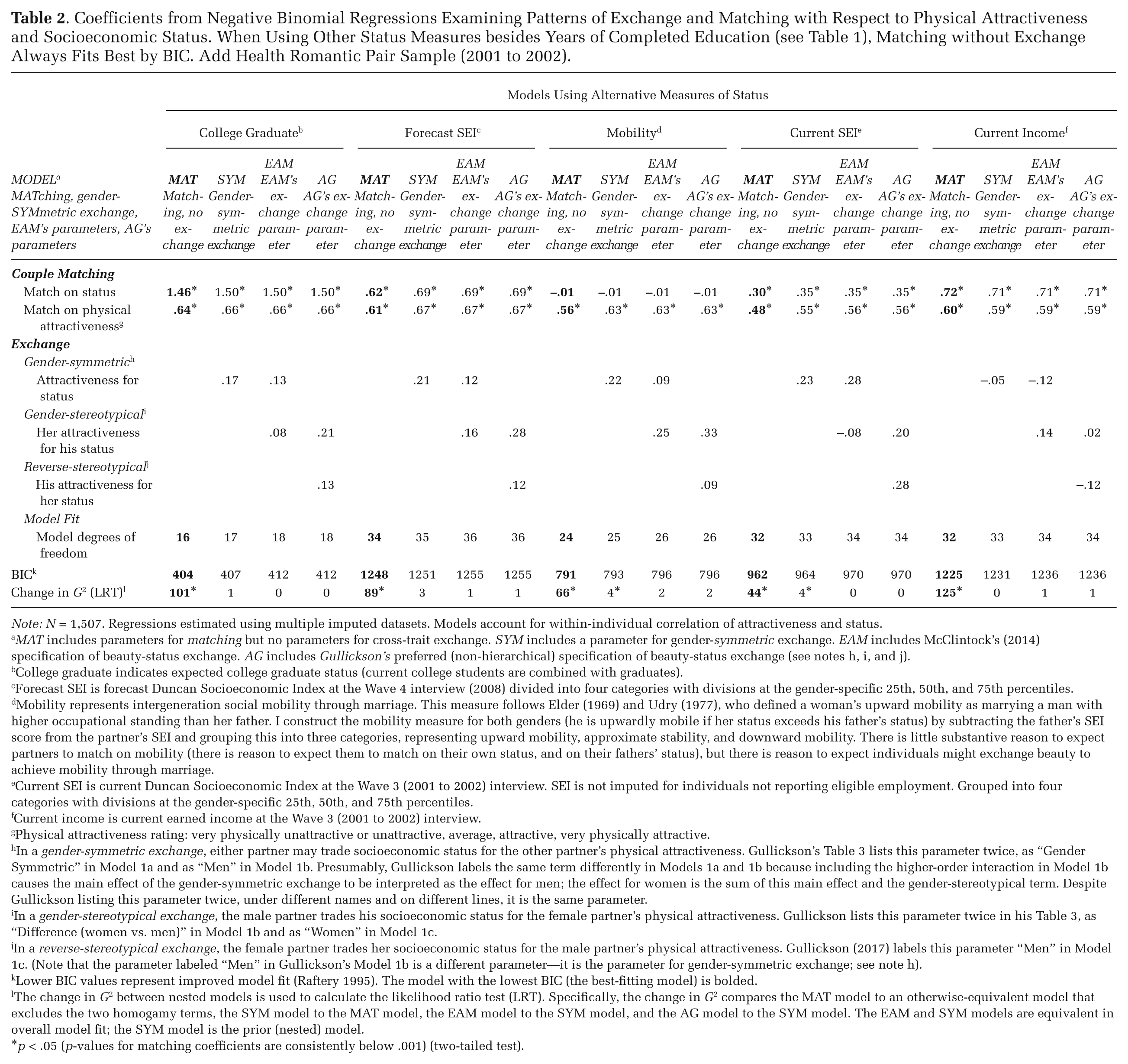
In my initial analysis, I considered six measures of socioeconomic status: years of completed education, expected college degree status, forecasted score on the Duncan Socioeconomic Index (SEI), socioeconomic mobility, current SEI score, and current earned income (for details, see McClintock 2014). Gullickson focuses on the only one of the six measures for which I found any evidence of gender-stereotypical beauty-status exchange, years of completed education. Accordingly, in Table 2, I present coefficients and model fit statistics from negative binomial regression models using Gullickson’s preferred model specification and the remaining five measures of socioeconomic status. Gullickson’s key result—a significant coefficient for gender-stereotypical beauty-status exchange—is entirely dependent on his choice of one specific measure of status.

Table 2.

Coefficients from Negative Binomial Regressions Examining Patterns of Exchange and Matching with Respect to Physical Attractiveness and Socioeconomic Status. When Using Other Status Measures besides Years of Completed Education (see Table 1), Matching without Exchange Always Fits Best by BIC. Add Health Romantic Pair Sample (2001 to 2002).

	Models Using Alternative Measures of Status
	College Graduate^b				Forecast SEI^c				Mobility^d				Current SEI^e				Current Income^f
MODEL ^a MATching, gender-SYMmetric exchange, EAM’s parameters, AG’s parameters	MAT Matching, no exchange	SYMGender-symmetric exchange	EAMEAM’s exchange parameter	AGAG’s exchange parameter	MATMatching, no exchange	SYMGender-symmetric exchange	EAMEAM’s exchange parameter	AGAG’s exchange parameter	MAT Matching, no exchange	SYMGender-symmetric exchange	EAMEAM’s exchange parameter	AGAG’s exchange parameter	MAT Matching, no exchange	SYMGender-symmetric exchange	EAMEAM’s exchange parameter	AGAG’s exchange parameter	MAT Matching, no exchange	SYMGender-symmetric exchange	EAMEAM’s exchange parameter	AGAG’s exchange parameter
Couple Matching
Match on status	1.46^*	1.50^*	1.50^*	1.50^*	.62^*	.69^*	.69^*	.69^*	–.01	–.01	–.01	–.01	.30^*	.35^*	.35^*	.35^*	.72^*	.71^*	.71^*	.71^*
Match on physical attractiveness^g	.64^*	.66^*	.66^*	.66^*	.61^*	.67^*	.67^*	.67^*	.56^*	.63^*	.63^*	.63^*	.48^*	.55^*	.56^*	.56^*	.60^*	.59^*	.59^*	.59^*
Exchange
Gender-symmetric^h
Attractiveness for status		.17	.13			.21	.12			.22	.09			.23	.28			–.05	–.12
Gender-stereotypicalⁱ
Her attractiveness for his status			.08	.21			.16	.28			.25	.33			–.08	.20			.14	.02
Reverse-stereotypical^j
His attractiveness for her status				.13				.12				.09				.28				–.12
Model Fit
Model degrees of freedom	16	17	18	18	34	35	36	36	24	25	26	26	32	33	34	34	32	33	34	34
BIC^k	404	407	412	412	1248	1251	1255	1255	791	793	796	796	962	964	970	970	1225	1231	1236	1236
Change in G² (LRT)^l	101^*	1	0	0	89^*	3	1	1	66^*	4^*	2	2	44^*	4^*	0	0	125^*	0	1	1

Note: N = 1,507. Regressions estimated using multiple imputed datasets. Models account for within-individual correlation of attractiveness and status.

College graduate indicates expected college graduate status (current college students are combined with graduates).

Forecast SEI is forecast Duncan Socioeconomic Index at the Wave 4 interview (2008) divided into four categories with divisions at the gender-specific 25th, 50th, and 75th percentiles.

Mobility represents intergeneration social mobility through marriage. This measure follows Elder (1969) and Udry (1977), who defined a woman’s upward mobility as marrying a man with higher occupational standing than her father. I construct the mobility measure for both genders (he is upwardly mobile if her status exceeds his father’s status) by subtracting the father’s SEI score from the partner’s SEI and grouping this into three categories, representing upward mobility, approximate stability, and downward mobility. There is little substantive reason to expect partners to match on mobility (there is reason to expect them to match on their own status, and on their fathers’ status), but there is reason to expect individuals might exchange beauty to achieve mobility through marriage.

Current SEI is current Duncan Socioeconomic Index at the Wave 3 (2001 to 2002) interview. SEI is not imputed for individuals not reporting eligible employment. Grouped into four categories with divisions at the gender-specific 25th, 50th, and 75th percentiles.

Current income is current earned income at the Wave 3 (2001 to 2002) interview.

Physical attractiveness rating: very physically unattractive or unattractive, average, attractive, very physically attractive.

In a gender-symmetric exchange, either partner may trade socioeconomic status for the other partner’s physical attractiveness. Gullickson’s Table 3 lists this parameter twice, as “Gender Symmetric” in Model 1a and as “Men” in Model 1b. Presumably, Gullickson labels the same term differently in Models 1a and 1b because including the higher-order interaction in Model 1b causes the main effect of the gender-symmetric exchange to be interpreted as the effect for men; the effect for women is the sum of this main effect and the gender-stereotypical term. Despite Gullickson listing this parameter twice, under different names and on different lines, it is the same parameter.

In a gender-stereotypical exchange, the male partner trades his socioeconomic status for the female partner’s physical attractiveness. Gullickson lists this parameter twice in his Table 3, as “Difference (women vs. men)” in Model 1b and as “Women” in Model 1c.

In a reverse-stereotypical exchange, the female partner trades her socioeconomic status for the male partner’s physical attractiveness. Gullickson (2017) labels this parameter “Men” in Model 1c. (Note that the parameter labeled “Men” in Gullickson’s Model 1b is a different parameter—it is the parameter for gender-symmetric exchange; see note h).

Lower BIC values represent improved model fit (Raftery 1995). The model with the lowest BIC (the best-fitting model) is bolded.

p < .05 (p-values for matching coefficients are consistently below .001) (two-tailed test).

For each of the five measures of socioeconomic status, the models presented in Table 2 parallel those presented in Table 1—the first models matching without exchange, the second models gender-symmetric exchange, the third model follows my specification of gendered exchange, and the fourth model follows Gullickson’s preferred specifications. If Gullickson’s results were robust, the coefficients on gender-stereotypical beauty-status exchange in the fourth model would be statistically significant, but they are consistently not significant.⁵ Moreover, across all five measures of socioeconomic status, the best-fitting model (that with the lowest BIC statistic) is the first model, which only accounts for matching. Evidence of beauty-status exchange is not robust to alternative measures of status, even using Gullickson’s preferred model specifications.

Discussion

Ultimately, Gullickson and I agree that there is some support for beauty-status exchange when measuring socioeconomic status as years of completed education. However, this support is not robust to alternative measures or model specifications. It is evident only for one of the six measures of socioeconomic status, completed years of education, a measure for which couple differences may be especially transient. Most subjects are in their early 20s, and age differences in young couples can create temporary inequality in completed education, particularly for students. Additionally, although Gullickson does not consider differences by union status, evidence that couples might trade years of completed education for beauty is strongest among dating couples and nonexistent among married couples. Finally, Gullickson’s preferred log-linear model specifications fail to improve model fit or to support beauty-status exchange when using alternative measures of socioeconomic status.

Empirical methodologists argue that an inference is not credible if it is fragile, if it can be reversed by minor changes to models or measures (Ioannidis 2005; Leamer 1985). To that end, my analyses included descriptive statistics, which have the advantage of simplicity and transparency; three forms of regression models, each imposing different assumptions; and six measures of socioeconomic status (I considered alternative measures of attractiveness in the online supplement). In revisiting my analyses, Gullickson makes methodological and conceptual arguments, but he fails to produce new or persuasive evidence. Gullickson’s critique of the difference models misconstrues the models’ conceptual appropriateness, and his modified difference models simply revert to another of my models in which there is evidence of exchange (the conventional regression models; McClintock 2014). Likewise, Gullickson’s alternative specification of beauty-status exchange in the log-linear models achieves a significant coefficient on the relevant parameter, but it fails to improve model fit and is entirely dependent on his choice of one specific measure of status. Using Gullickson’s preferred measure of beauty-status exchange and substituting any of the remaining five measures of socioeconomic status (Table 2) produces no support for gender-symmetric or gender-stereotypical beauty-status exchange.

The fragility of support for beauty-status exchange, whether gender-symmetric or gender-stereotypical, demonstrates the importance of seeking robust results, rather than seeking support for a given theory (Ioannidis 2005). This is especially imperative when a theoretical perspective has attained canonical acceptance—good science questions widely-shared assumptions, and a theory as generally accepted as gender-stereotypical beauty-status exchange should evidence robust support. My analysis used a range of credible and theoretically motivated models and measures, and I found little support for beauty-status exchange, as conceptualized in the relevant literature. Doubtless, beauty-status exchange sometimes occurs, but in this sample of young couples, it is not a common pattern of partner selection. Instead, the overwhelming tendency is for couples to match on physical attractiveness and socioeconomic status.

Footnotes

Acknowledgements

I would like to thank Michael J. Rosenfeld, Abigail R. Ocobock, Jessica L. Collett, and Erin McDonnell for their helpful comments on this article. Their advice has been invaluable.

Data

This research uses data from Add Health, a program project designed by J. Richard Udry, Peter S. Bearman, and Kathleen Mullan Harris, and funded by a grant P01-HD31921 from the National Institute of Child Health and Human Development, with cooperative funding from 17 other agencies. Special acknowledgment is due Ronald R. Rindfuss and Barbara Entwisle for assistance in the original design. Persons interested in obtaining data files from Add Health should contact Add Health, Carolina Population Center, 123 W. Franklin Street, Chapel Hill, NC 27516-2524 (addhealth@unc.edu).

Editors’ Note

To avoid any possible conflict of interest, the entire review process for this article was handled by an ASR Deputy Editor with no Notre Dame affiliation.

1.

Gullickson’s model is misspecified, in that it excludes appropriate lower-order terms (). Gullickson’s beauty-status exchange terms are not hierarchically nested, whereas I nest gender-stereotypical exchange within the lower-order interaction, gender-symmetric exchange. Strictly speaking, gender-stereotypical beauty-status exchange is an interaction of educational hypergamy (he is more educated) and physical attractiveness hypogamy (he is less attractive), so these lower-order terms should also be included. However, including hypergamy and hypogamy parameters does not substantively alter the results, nor does it improve model fit.

2.

For the purposes of model fit, my specification of gendered beauty-status exchange and Gullickson’s specification are equivalent. The models differ in their ability to detect significant gender differences, but they use the same degrees of freedom and predict identical cell counts.

3.

Modeling similarity in the education and attractiveness of non-matched couples lowers the BIC to 1098 (differing by one level of attractiveness or education is more common than differing by two levels, and differing by three levels is least common). Allowing the strength of educational matching to vary by educational level further lowers the BIC to 1069 (matching is strongest among college graduates).

4.

Compared to the model that only includes gender-symmetric exchange (SYM), Gullickson’s preferred model raises the BIC by 4.

5.

Even if one removes the term for reverse-stereotypical exchange, the term representing gender-stereotypical exchange remains statistically insignificant for these five measures of status (not shown).

Elizabeth Aura McClintock is an Assistant Professor of Sociology at the University of Notre Dame. Her research addresses how intimate relationships reflect, perpetuate, and potentially alter gender, class, age, and racial inequalities. Recent publications examine the association of women’s and men’s occupational sex composition with romantic and relationship outcomes, such as the gendered division of housework. Methodologically, much of her research considers how researchers’ preconceptions and biases, such as commonly held gender stereotypes, may influence research questions, study design, and interpretation of results.

References

Agresti

Alan

. 1996. An Introduction to Categorical Data Analysis. New York: John Wiley & Sons.

Elder

Glen H.

1969. “Appearance and Education in Marriage Mobility.” American Sociological Review 34(4):519–33.

Gullickson

Aaron

. 2017. “Comments on Conceptualizing and Measuring the Exchange of Beauty and Status.” American Sociological Review 82(5):1093–1099.

Ioannidis

John P. A.

2005. “Why Most Published Research Findings Are False.” PLoS Medicine 2(8):696–701.

Ioannidis

John

Doucouliagos

Chris

. 2013. “What’s to Know About the Credibility of Empirical Economics?” Journal of Economic Surveys 27(5):997–1004.

Kalmijn

Matthijs

. 2010. “Educational Inequality, Homogamy, and Status Exchange in Black-White Intermarriage : A Comment on Rosenfeld.” American Journal of Sociology 115(4):1252–63.

Leamer

Edward E.

1983. “Let’s Take the Con Out of Econometrics.” American Economic Review 73(1):31–43.

Leamer

Edward E.

1985. “Sensitivity Analyses Would Help.” American Economic Review 75(3):308–313.

Long

Scott J.

Freese

Jeremy

. 1997. Regression Models for Categorical Dependent Variables Using Stata. College Station, TX: Stata Press.

10.

McClintock

Elizabeth Aura

. 2010. “When Does Race Matter? Race, Sex, and Dating at an Elite University.” Journal of Marriage and Family 72(1):45–72.

11.

McClintock

Elizabeth Aura

. 2014. “Beauty and Status: The Illusion of Exchange in Partner Selection?” American Sociological Review 79(4):575–604.

12.

McClintock

Elizabeth Aura

. 2017. “Occupational Sex Composition and Gendered Housework Performance: Compensation or Conventionality?” Journal of Marriage & Family 79(2):475–510.

13.

Raftery

Adrian E.

1986. “Choosing Models for Cross-Classifications.” American Sociological Review 51(1):145–46.

14.

Raftery

Adrian E.

1995. “Bayesian Model Selection in Social Research.” Sociological Methodology 25:111–63.

15.

Rosenfeld

Michael J.

2005. “A Critique of Exchange Theory in Mate Selection.” American Journal of Sociology 110(5):1284–1325.

16.

Rosenfeld

Michael J.

2010. “Still Weak Support for Status-Caste Exchange: A Reply to Critics.” American Journal of Sociology 115(4):1264–76.

17.

Schwartz

Gideon E.

1978. “Estimating the Dimension of a Model.” Annals of Statistics 6(2):461–64.

18.

Udry

J. Richard

. 1977. “The Importance of Being Beautiful: A Reexamination and Racial Comparison.” American Journal of Sociology 83(1):154–60.

Support for Beauty-Status Exchange Remains Illusory

Abstract

Keywords

Overview

Difference Models

“Confounding” Floor and Ceiling Effects?

Log-Linear Models

Alternative Specifications of Beauty-Status Exchange

Union status

Model fit. 2

Measuring Socioeconomic Status

Discussion

Footnotes

Acknowledgements

Data

Editors’ Note

1.

2.

3.

4.

5.

References

Model fit.²