Crime concentrations and micro places: An empirical test of the “law of crime concentration at places” in Belgium

Abstract

This study examines the extent to which crime concentrations occur at micro places, in order to test Weisburd’s law of crime concentration at places, in two large Belgian cities. Police-registered crime data for the period 2004–2012 were used. Analyses were conducted at the grid level (using 200 meters by 200 meters grid cells), as a proxy for behavior settings. This study assesses Weisburd’s theoretical proposition and by (partly) replicating prior empirical research, we conclude that the findings are in line with those from prior studies regarding crime concentration at micro places. Finally, opportunities and avenues for future research on crime places are discussed.

Keywords

Crime statistics environmental criminology grid cells law of crime concentration micro places

Introduction

Micro places are small geographical locations that in recent years have gained increasing prominence in empirical research in the field of environmental criminology. The criminology of place focuses primarily on these micro-units of analysis, such as addresses, street segments, or clusters of these units (Weisburd, Bruinsma, & Bernasco, 2009). When reviewing the existing literature on the criminology of place, it is immediately clear that these micro-units often have disparate definitions, and hence, they are operationalized differently too. For example, Sherman, Gartin, and Buerger (1989) define a “place” as: “a fixed physical environment that can be seen completely and simultaneously, at least on its surface, by one’s naked eyes” (p. 31), while Eck and Weisburd (1995) define micro places as “specific locations within the larger social environment” (p. 3). As stated by Payne (2018): “The definition of ‘place’ often depends on the research question and on pragmatic concerns such as data availability and degree of error in the data” (p. 146). Madensen and Eck (2013) bring conceptual clarity and provide a theoretical meaningful distinctions among place aggregations by distinguishing (1) proprietary places,¹ (2) proximal places,² and (3) pooled places.³

Within environmental criminology in general and the criminology of place in particular the focus is not so much on the “why” of deviant behavior as on why concentrations of crime arises “in specific places and at specific times.” This tradition has its origins in diverse urban traditions: it combines aspects of situational crime prevention (Weisburd, Bernasco, & Bruinsma, 2009), urban planning and urban design (for urban design, see Jeffery, 1971), and urban architecture (see Newman, 1972). As a result, features of physical space and criminal opportunity (Eck & Weisburd, 1995) also acquire a place alongside the much more established social ecology (Byrne & Sampson, 1986; Reiss & Tonry, 1986; Wikström, 2007), which placed significantly more emphasis on neighborhoods (higher aggregation levels than micro places) as breeding grounds or magnets for crime concentrations and fear of crime (Covington & Taylor, 1991).

One of the main findings from research within the criminology of place is that crime is concentrated within a relatively limited number of micro places (Weisburd, 2015; Wilcox & Eck, 2011). Repeated assertions concerning crime concentrations in different contexts have resulted in the formulation of a universal law, also called the law of crime concentration at places. This law has so far been tested mainly, but not exclusively, in the context of the United States (Lee, Eck, SooHyun, & Martinez, 2017; Telep & Weisburd, 2018). In this contribution we will examine whether this law of crime concentrations also applies at the level of micro places in a West European context. As Favarin (2018) states: “the generalizability of the law of crime concentration is missing important information pertaining to non-US cities, especially in Europe” (p. 3). As social laws are supposed to have a general nature and thus applicable in different context, every additional test informs us of the robustness of the relationship. Additionally, every new test may be seen as a potential falsifier of the theory (Bruinsma & Pauwels, 2018; Opp, 2014). In this light, it might be interesting for readers on the other side of the world (e.g. New Zealand) to read about a test in an unprecedented context with an unconventional operationalization of micro places.

The structure of this contribution is as follows. We start with an outline of Weisburd’s proposition. Then, we provide a nonexhaustive overview of studies on the so-called law of crime concentration at places. Next, we discuss the aims of our study, the data and methods used, and the results. We conclude by asking what this contribution means for (future) empirical research within the criminology of place.

Weisburd’s propositions on the law of crime concentration at places

As will be set out in the next section, there is strong empirical evidence that crime is not proportionally and randomly distributed across (micro) places. Regarding the concentration of crime at micro places, Weisburd (2015) postulated a series of propositions with the aim to give an impetus to the policy regarding crime control and the etiology of the criminology of place; to unravel the crime–place connection to say it in his own words (Weisburd & Eck, 2018).

The search after a general law was the starting point of the study of Weisburd, Groff, and Yang (2012; Telep and Weisburd, 2018). In this study, Weisburd et al. (2012) came to five conclusions based on their longitudinal research on crime concentrations in Seattle, Washington, which indicate the importance of micro places:

Crime is highly concentrated at so-called hot spots, that is to say, a small number of places is responsible for a large proportion of crime (cf. Sherman et al., 1989).

The concentration of crime is consistent over time and crime is also concentrated in the same places.

Crime is highly variable at the micro level; the use of higher aggregation levels results in a loss of information.

Crime is not the only factor to vary significantly at the micro level; social and contextual characteristics of places also vary at the micro level.

Crime relating to space is predictable and this makes it possible, in addition to understanding crime concentrations, to adopt effective prevention strategies at the hot spots in question.

Thereafter, in 2015, Weisburd formulated his general law of crime concentration at places: “for a defined measure of crime at a specific microgeographic unit, the concentration of crime will fall within a narrow bandwidth of percentages for a defined cumulative proportion of crime” (p. 138). Essentially, the law claims that for specific types of crime a limited range of percentages of micro places will be responsible for a specific concentration of crime (e.g. 25 or 50% of the crime in a city). The emphasis on the type of crime is important, given that the concentration of crime differs to the extent that other crime types are studied.

Weisburd (2015) goes on to maintain:

I have focused on a first law of the criminology of place - the law of crime concentration at places. I have presented new evidence showing that the law applies with startling consistency both across cities and within cities across time. The data suggest that the law of crime concentration is a “general proposition of universal validity” (Sutherland, 1947:23), analogous to physical laws observed in the natural sciences. (p. 151)

This is what Popper would have called a “bold statement”: general validity is a strong claim, which calls for replication studies in multiple cultural settings. The concept of “law” should not be interpreted as a covering law (Hempel, 1963). However, descriptive empirical social laws raise questions. Such descriptions require an adequate explanation of the conditions and mechanisms behind the empirical law (see Bruinsma & Pauwels, 2018 for a discussion).

Since 2015, this law of crime concentration is increasingly being studied within the criminology of place tradition. First, Weisburd et al. (2016) have concretized the general law by setting the threshold for 50% of crime at approximately 4% of the micro places and 25% of crime at less than 1.5% of the micro places.

Later, Bernasco and Steenbeek (2017) state that the criminology of place “has not yet developed common standards for reporting and summarizing crime concentrations” (p. 452) and the law of crime concentration does not close this gap, because this law does not prescribe how crime concentration at places should be measured. Using cumulative percentage statements, as the definition of the law hints to, results in using defined cutoff values, such as 25 or 50% of crime in a city, which are arbitrary (Lee, 2017). In order to overcome this, Bernasco and Steenbeek (2017) advocate showing the entire cumulative distribution. They recommend the use of the (standardized) Lorenz curve and the (standardized) Gini coefficient when reporting and summarizing crime concentrations (Bernasco & Steenbeek, 2017). The Lorenz curve is a representation of the cumulative distribution of a variable (e.g. crime, operationalized as the number of crime incidents or calls for service) compared to the cumulative distribution of units of analysis (e.g. places, operationalized as street segments or grid cells). Bernasco and Steenbeek (2017) emphasize the added value of the Lorenz curve:

Applied to the distribution of crimes across places, the Lorenz curve plots cumulative percentages of crime on the vertical axis against cumulative percentages of places on the horizontal axis, with the places ordered by number of crimes. Thus, each and every point on the curve corresponds to a statement like “Y percent of crimes occur in the X percent most targeted places”. In other words, the Lorenz curve includes in a single graph all cumulative percentage statements that can be made about a given crime distribution! By presenting the Lorenz curve there is no longer any need to decide on a cut-off value for X or for Y, as all are included. (p. 4)

The Gini coefficient is a number that expresses the degree of concentration in a distribution. This coefficient summarizes the concentration using a numeric value. The Gini coefficient was designed more than a century ago in order to express the degree of income inequality. A value 0 corresponds to “perfect equality,” in this case the absence of crime concentrations or with other words: an equal number of crimes are committed in all places. A value of 1 corresponds to “perfect inequality,” in this case maximum concentration of crime or with other words: all crimes are committed in a single place.

The use of the Lorenz curve and the Gini coefficient is problematic when there are fewer crimes than units of analysis, because this results in an overestimation of the level of crime concentration as an equal distribution of crime across places is theoretically not possible (Bernasco & Steenbeek, 2017; Sherman et al., 1989). In these cases—when crime would still not be concentrated in all places, even if there would be a perfectly equal distribution of crime across the units of analysis—Bernasco and Steenbeek (2017) recommend the use of a standardized Lorenz curve and a standardized Gini coefficient (G′).

Besides these reporting standards, other statistics are also available. In his doctoral dissertation, Lee (2017) compares measures of the concentration of crime at places and times. Regarding crime at place, he compares the decile index, Gini index, Shannon index, and Simpson index. He concludes that, for reporting spatial concentration of crime, the use of the Shannon index is often preferred. Curiel and Bishop (2016) propose the use of the Rare Event Concentration Coefficient, especially in cases that—as the name suggests—events are rare. This coefficient is mixture model based on a Poisson distribution.

Prior empirical research

Empirical research within the criminology of place has demonstrated for decades that crime concentrates at (micro) places. Thirty years ago, as far back as 1989, Sherman et al. already discovered that there were strong concentrations of crime at a very limited number of places in a city. For example, Sherman et al. (1989) discovered that in Minneapolis (Minnesota) only 3.3% of places were responsible for 50.4% of calls to the police (N = 323,979). This concentration was even pronouncedly greater when they were examined for separate types of crime. For example, it appeared that for robbery (N = 4166), auto theft (N = 3908), and criminal sexual conduct (N = 1729), respectively, 2.2, 2.7, 1.2% of all places (i.e. approximately 115,000 addresses) were responsible for 100% of all calls to the police regarding the respective types of crime.⁴

This finding was a major impetus which boosted a lot of enquiries into crime concentrations at micro places. Since the late 1980s, various studies have reported a significant concentration of crime at micro places in various cities across the United States (Braga, Hureau, & Papachristos, 2010; Pierce, Spaar, & Briggs, 1988; Weisburd, 2015; Weisburd, Bushway, Lum, & Yang, 2004). It is only recently that similar studies have appeared outside the United States. Andresen and Malleson (2011) studied crime concentrations in Vancouver (Canada), Andresen and Linning (2012) in Ottawa (Canada), Weisburd and Amran (2014) in Tel Aviv (Israel), Melo, Matias, and Andresen (2015) in Campinas (Brazil), Steenbeek and Weisburd (2015) in The Hague (the Netherlands), Vandeviver and Steenbeek (2017) in Antwerp (Belgium), and Favarin (2018) in Milan (Italy). Recently, Lee et al. (2017) carried out a review that covered 44 studies, of which nine were analyzed regarding the prevalence of crime concerning a non-U.S. context, including some of those listed above. These scholars unanimously reached the same conclusion: crime at the micro place level is not proportionately distributed across the micro-units of analysis in question.

In the Belgian context, Vandeviver and Steenbeek (2017) recently tested the law of crime concentration at places in Antwerp, Belgium for residential burglary at street segments⁵ from 2005 to 2016. They found that 50% of the crime incidents concentrate (on a yearly basis) between 1.83 and 2.55% of the street segments.⁶ The basic descriptive statistics mentioned in Vandeviver and Steenbeek’s (2017) study indicate that major European cities do not have a gridiron plan like major cities in the United States and, as a consequence, street segments are highly variable in their lengths.⁷ This conclusion is an important one, as it demonstrates the importance of the replication of the test in different contexts.

The purpose of this study

The purpose of this study is to test Weisburd’s law of crime concentration at places and concomitantly (partly) replicate⁸ prior empirical findings regarding crime concentration at micro places in the Belgian urban context, which has a different geographical, functional, and morphological structure from the urban context in the United States. We perform a test of the law of crime concentration at places with other units of analysis than the frequently used street segments, however, with micro-geographic units of analysis and therefore partly replicate prior empirical findings. We test this geographical law by using state-of-the-art reporting and summarizing standards (see Bernasco & Steenbeek, 2017).

Our intent for this test is to empirically study whether crime concentrations at micro places are present in two major Belgian cities. Although the question is descriptive, the results contribute to increasing our knowledge concerning the generalizability of the descriptive law. In addition, we submit that this test may be an additional step at the forefront of unraveling the crime–place connection (Weisburd & Eck, 2018) for several reasons. First, the use of unconventional—but nevertheless still micro geographic—units of analysis as an operationalization of micro places and, second, the comparison of three different types of crime within two major urban cities is unprecedented in an European context. Third, we study the temporal stability of these findings.

Operationalization of micro places

Studies on the social ecology of crime and environmental criminological research are often based on geographical units that are mainly set up for administrative purposes. However, the analysis of crime data in excessively large geographical units can mask geographical variability, which is present on a lower level (Albert J. Reiss Jr., personal communication in Sherman et al., 1989; Gerell, 2017, Stark, 1987). This can have implications for the validity of the findings. Excessive research and reflections of scholars taught us that smaller units of analysis are better (Oberwittler & Wikström, 2009). A vast amount of the variance in crime incidents can be attributed to the micro level when compared to larger units of analysis (O’Brien & Winship, 2017; Schnell, Braga, & Piza, 2017), so the action in crime is definitely at the micro place level (Steenbeek & Weisburd, 2015).

When formulating his law, Weisburd (2015) did not operationalize micro places in the formal definition, although he hints the use of street segments as he used the street segment as a unit of analysis in the empirical part of the same contribution. A street segment is defined as the part of the street that is situated between two intersections. In the cities studied in the United States there are city blocks, which means that the street segments are—in general—of comparatively equal length. This typical gridiron plan in major cities in the United States makes this a user-friendly level of analysis in this context. Major European cities—as described earlier—do not have such a gridiron plan, which means that street segments are of highly variable lengths. It therefore makes sense that longer street segments would have a higher likelihood of crime concentrations than shorter street segments.

We argue that, with regard to the study of crime concentrations, another operationalization of a micro place (i.e. a grid cell) may better suit the morphology of the cities studied, as a plausible alternative for street segments. The grid level is created by spreading a uniform grid over a geographical area. These grid cells can have several dimensions, but in this study we used grid cells of 200 meters by 200 meters. This unit of analysis is already used on a small scale for projects and is likely to gain importance in the future (e.g. Rummens, Hardyns, & Pauwels, 2017). Following Wikström, Oberwittler, Treiber, and Hardie (2012), Bernasco, Bruinsma, Pauwels, and Weerman (2013) argue that small grid cells (200 meters by 200 meters) can be seen as “behavior settings.” These are small areas where people may choose to commit crimes, based on the temptations, provocations, signaling cues and deterrence levels.

One advantage of the grid level compared to the street segment level is that grid cells have fixed dimensions, whereas this is not the case for street segments. Hence, it standardizes the content from a geographical point of view. This might be advantageous regarding the extent of biased outcomes due to the choice for an aggregation level. This problem is known as the modifiable areal unit problem (MAUP) (see Openshaw, 1984). The MAUP, or the problem concerning the scalability of spatial units, demonstrates the difficulty in choosing the appropriate aggregation level (Dark & Bram, 2007). The core element of this problem is that identical data, which are aggregated in various ways, can lead to different results. MAUP involves both the issue concerning which aggregation level is the most appropriate in a specific study (zonation effect) and the issue of how to aggregate data to a higher aggregation level (scale effect) (Oberwittler & Wikström, 2009). By using very small geographical units of analysis, we try to minimize the MAUP.

Data and methods

Data

In this study, registered police data from two major Belgian cities⁹ spanning nine years (2004–2012) were used. Both cities are among the largest cities in Belgium with more than 150,000 inhabitants. The data were geocoded at the grid level. Grid cells of 200 meters by 200 meters were used. City X and Y have, respectively, 5403 and 4254 grid cells. Three crime types were studied separately: residential burglary,¹⁰ assault and battery,¹¹ and aggravated robbery.¹²

For each crime type the accuracy of the indicated location has been verified (see Table 1). The quality of geographical research depends on the methodological issues that may arise at the geographical level: the number of correctly completed police records including an indication of place varies significantly for the different types of crime and the geocoded information is more accurate for crime types involving a static target than for crime types involving a mobile target. In the case of unidentifiable street names, we unfortunately have no other option than to delete these cases from the dataset. For missing house numbers, we looked for a suitable and methodologically defensible method of allocation (on a grid) in order to retain as many data as possible for the analyses.¹³ An overview of the missing data for City X and City Y can be found in Table 1.

Table 1.

Accuracy of the location, City X and City Y, 2004–2012.

	N	Missing street	Missing house number
City X
Aggravated robbery
Theft including violence	11,003	2.0% (221)	67.5% (7424)
Theft including weapon	3490	2.2% (77)	52.1% (1820)
Purse theft	4545	1.2% (54)	69.0% (3138)
Assault and battery	52,727	1.0% (536)	36.4% (19,195)
Residential burglary	43,901	0.2% (70)	2.0% (878)
City Y
Aggravated robbery
Theft including violence	3501	2.9% (103)	58.9% (2.061)
Theft including weapon	206	1.5% (3)	18.0% (37)
Purse theft	1299	1.0% (13)	66.1% (859)
Assault and battery	29,035	4.6% (1.339)	37.3% (10.837)
Residential burglary	13,567	0.7% (90)	2.7% (370)

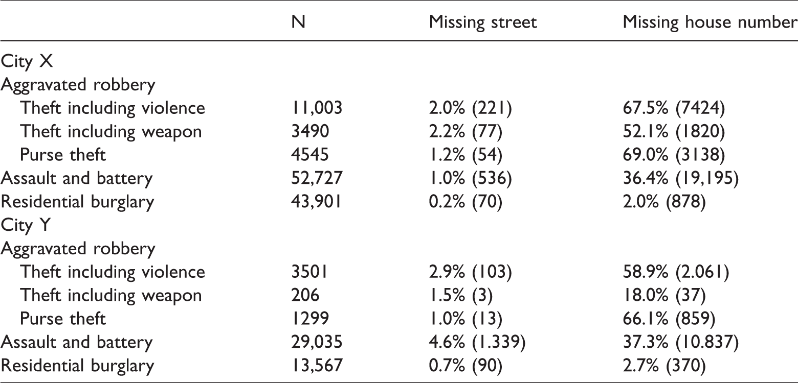
Table 1 shows that a missing house number is a more frequent problem than a missing street. In the case of missing streets, the variation ranges from 0.2 to 2.2% for City X and from 0.7 to 4.6% for City Y. In the case of a missing house number, the variation ranges from 2.0 to 69.0% for City X and from 2.7 to 66.1% for City Y. A missing house number seems to depend on the nature of the target (mobile versus static): in the case of residential burglaries it is for the most part inherent to the event that the house number is known. Yet, here we can report a certain amount of incomplete registrations too.

Methods

Both overall crime concentrations across the nine years studied and the annual variances in crime concentrations are calculated. To compare the results of our study with prior research, cutoff values are reported and in addition, in accordance with recently recommended reporting and summarizing standards, the Lorenz curve and Gini coefficients are reported as well. For the formula used to calculate the (standardized) Gini coefficient, we refer to Bernasco and Steenbeek (2017).

Results

In this section, the crime concentrations for three different types of crime on the grid level in two major Belgian cities are described. When calculating concentration measures, grid cells without crimes (i.e. zero counts) were included, because the absence of crime at certain places is an important element of its distribution. In other words, in this study crime concentrations are addressed in terms of prevalence and not in terms of frequency (Lee et al., 2017). For other purposes, it might be useful to use a different procedure (i.e. calculating concentrations among places that suffered at least one crime incident).

Overall crime concentrations in nine years

First, the overall crime concentration in nine years (2004–2012) is described. The amount of grid cells per city is lower than the crime count per crime type over nine years in the respective cities and, as a consequence, no correction has to be made at the calculations of the summary statistics (i.e. Lorenz curve and Gini coefficient). For the crime types aggravated robbery, assault and battery, and residential burglary, City X counts, respectively, 18,518; 51,848; and 43,760 registered crime incidents and City Y counts, respectively, 4723; 27,496; and 13,410 registered crime incidents.

Figure 1 illustrates the percentage of all grid cells in which, respectively, 25 and 50% of the crime incidents are concentrated. The bars in Figure 1 indicate the percentage of grid cells in which the given percentage of crime incidents is located, hence, lower percentages (and thus lower bars) indicate higher levels of crime concentration. The left side of Figure 1 contains the levels of concentration of 25% of the crime incidents. The right side of Figure 1 contains the levels of concentration of 50% of the crime incidents.

Figure 1.

The law of crime concentration at places per crime type at the grid level (2004–2012).

The differences between the crime types and cities are remarkable. The concentrations in City Y are, in general, slightly higher than in City X; however, the ratios between the crime types in both cities remain the same. There are obvious differences in the levels of crime concentration across the different types of crime. The concentration of aggravated robbery incidents is the strongest for both cities, followed by the concentration of assault and battery incidents. The concentration of residential burglaries is the weakest from the three crime types; however, these crime incidents are still concentrated in a small number of grid cells.

The cutoff values used in Figure 1 (i.e. 25 and 50% of crime incidents) are frequently used in prior research regarding (the law of) crime concentrations within the criminology of place. However, as recently stated by Bernasco and Steenbeek (2017), these cutoff values might be arbitrary and definitely do not provide an overview of the total distribution. Therefore, in Figure 2, the Lorenz curve contains the total distribution of crime concentrations for the distinct crime types and the two cities.

Figure 2.

Lorenz curve of crime data (2004–2012) at the grid level.

Figure 2 shows the distribution of the crime concentration by visualizing the cumulative percentage of places (on the x-axis) compared to the cumulative percentage of crime incidents (on the y-axis). This visualization clearly demonstrates that crime incidents at the grid level are highly concentrated in a few places. This visualization of the distribution of the crime concentrations also provide visual evidence that the range of percentages of micro geographic units (i.e. the “bandwidth”; Weisburd, 2015) is very narrow for several specific cumulative proportions of crime.

To summarize the distribution of the crime concentrations visualized in Figure 2, the Gini coefficient is calculated for the three different crime types and two cities. These Gini coefficients are visualized in Figure 3, where higher bars indicate a higher Gini and, hence, implicate a stronger concentration of crime incidents. Based on these Gini coefficients, the same conclusions can be drawn as previously based on the cutoff values, however; these coefficients summarize the distribution as a whole: the concentration of aggravated robbery incidents is the strongest, followed by assault and battery incidents, and finally the residential burglaries. Generally, the crime concentrations across the three crime types in City Y are slightly stronger than in City X.

Figure 3.

(Unstandardized) Gini (G) coefficients per crime type for City X and Y.

Stability of crime concentrations across years

In addition to the overall crime concentrations between 2004 and 2012, the stability of the crime concentrations across these nine years is assessed. By calculating the crime concentration per crime type and per year, the amount of grid cells per city is frequently higher than the crime count (see Figure 5, 6 and 7 in Appendix 1). As a consequence, corrections have to be made at the calculation of the summary statistic used. In this section, we report the standardized Gini coefficient (G′). In cases where the crime count is equal to or higher than the amount of grid cells per city, the standardized Gini (G′) coefficient equals the unstandardized Gini (G) coefficient (Bernasco & Steenbeek, 2017, p. 459).

The bars in Figure 4 illustrate the percentage of all grid cells (on the primary y-axis) in which 50% of the crime incidents are concentrated for respective City X and Y (note that lower percentages are visualized by lower bars and indicate higher levels of crime concentration). However, as places outnumber crimes in most of the years, perfect equality is not logically possible for these cases and, as a consequence, reporting these statistics would be inappropriate. For this reason, we added the standardized Gini (G′) coefficient as lines (on the secondary y-axis) in Figure 4.

Figure 4.

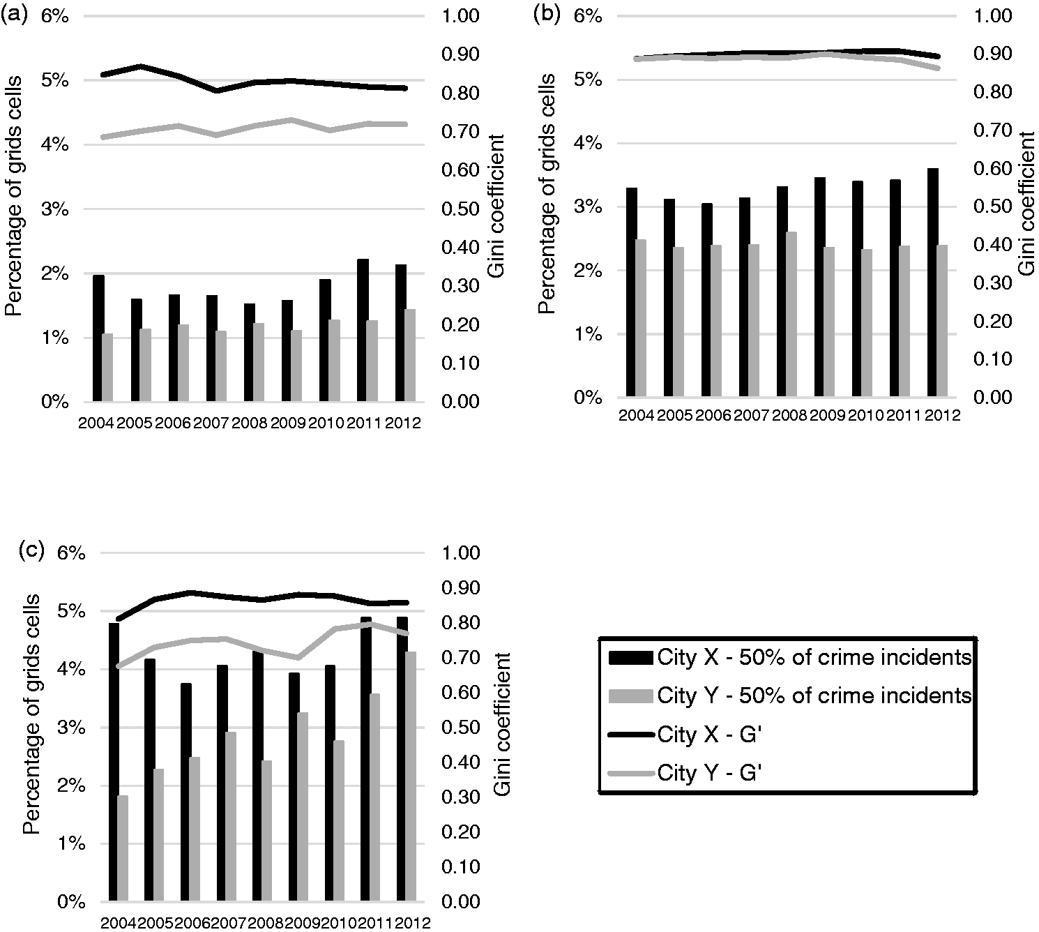
Standardized Gini (G′) coefficients and 50% cutoff values per crime type per year for City X and Y. (a) Aggravated robbery, (b) Assault and battery, and (c) Residential burglary.

Figure 5.

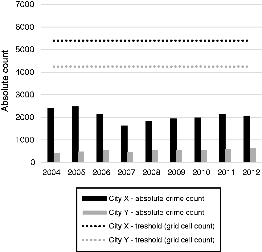
Assessment of the number of grid cells per city compared to the number of aggravated robbery incidents per city per year.

Figure 6.

Assessment of the number of grid cells per city compared to the number of assault and battery incidents per city per year.

Figure 7.

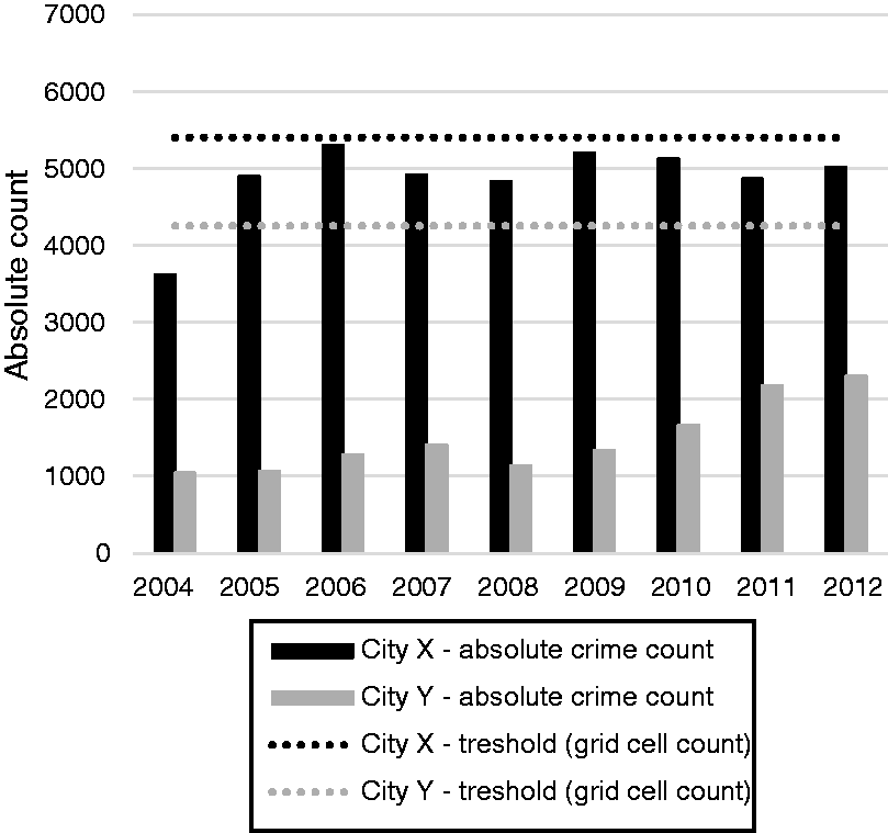
Assessment of the number of grid cells per city compared to the number of residential burglary incidents per city per year.

As can be observed, in cases where data are very scarce (e.g. in the case of aggravated robbery in City Y) the downward correction by the standardized Gini coefficient is significant. In cases where the correction of the Gini coefficient actually was not necessary for every individual year (e.g. in the case of assault and battery in City X), the standardized Gini is very high (e.g. assault and battery in City X has an average G′ of 0.90).

When the trends for the crime concentrations of the different crime types in Figure 4 are compared to each other, it becomes immediately clear that some crime types display stronger annual fluctuations in crime concentrations than others. In particular, residential burglary displays a strong annual variety, both in the cutoff values (displayed in bars) as in the Gini coefficients (displayed in lines). The two remaining crime types (i.e. aggravated robbery, and assault and battery) show more stable trends in crime concentrations across nine years.

Conclusion and discussion

In this study, crime concentrations at places were studied in two major Belgian cities from the standpoint of Weisburd’s law of crime concentration. By doing this, prior research regarding crime concentration in urban settings was partially replicated. With regard to the overall crime concentrations in nine years, the results are aligned with prior empirical findings concerning crime concentrations at micro places (e.g. with those of Weisburd (2015) and Lee et al. (2017)). It was found that 25% of crime is concentrated according to crime type and according to the city between 0.44 and 1.86% of the micro places, with 50% of crime concentrated between 1.61 and 5.37% of the places. These results are based on a period of nine years (2004–2012). Looking at the (arbitrary) cutoff values, remarkable differences between the different crime types and respective cities were observed, as the concentrations of crime in City Y tend to be stronger than crime concentrations in City X. In addition, residential burglaries tended to be more dispersed than the other types of crime. This indicates that combining different crime types into a single crime concentration index may hide significant variances or mask more specific crime patterns for each and every crime type. Using contemporary recommended reporting and summarizing standards, it was concluded that the Lorenz curve, which shows the full distribution of crime, visualize the very narrow bandwidth of relative frequencies of places in which crimes concentrate. This strong concentration was also indicated by the Gini coefficient, which was observed to vary across crime types and across cities between 0.85 and 0.94 during 2004 and 2012. As for the stability of crime concentrations across years, the results indicated that the extent of the fluctuations in crime concentrations across years was not equal for the three crime types. In particular, again, residential burglary displayed a different pattern unlike the other types of crime.

We argued that it is also important to consider grid cells as micro places because they can be seen as behavioral settings from a theoretical point of view (Bernasco et al., 2013; Oberwittler & Wikström, 2009). From a methodological perspective, the street segment level might be less useful in European cities, such as Belgian cities, than in the urban U.S. context, given their specific morphology (which from a geographical perspective seem to compare more or less to the smaller, nonmetropolitan U.S. cities). However, additional research is needed to ascertain at the empirical level to what extent the street segment level is applicable and what the implications are for classification on the basis of these micro places.

The street segment is a very relevant micro level in studying crime, given its importance in

organizing the daily lives of city dwellers and because they are a small enough spatial unit of analysis to minimize aggregation bias while large enough to ensure having a measurable number of burglaries and detecting meaningful changes in spatial patterns of burglary. (Vandeviver & Steenbeek, 2017, p. 6)

Or as Weisburd, Shay, Amram, and Zamir (2018) state: “Street segments are the building blocks of social life in cities” (p. 113). Moreover, one could argue that grids standardize space, but not its content or included proprietary places (cf. Madensen & Eck, 2013). In other words, grid cells do contrast the prior efforts to define places with an ontological meaning. With this study, we are not able to contradict this, as the aim was to describe crime concentrations in order to see to what extent the micro place disparities follow Weisburd’s law of crime concentration in two urban contexts and over nine years.

It is important not only to focus on the concentration of crime at place, but additionally on the causal mechanisms behind the law of crime concentration (Bruinsma & Pauwels, 2018). One of the next steps is to open the black box (Parri, 2014). To obtain this goal, integrated theory is required and the question must be asked as to why specific interactions and acts of crime take place in certain micro places. Micro places are, after all, not real actors of flesh and blood, but small entities that trigger decision processes (Wortley, 2001). A real explanation will therefore undoubtedly require a complex macro–micro–macro integration (Opp, 2011). A productive way of evaluating explanations may be the development of a research program of integrated theory comparison that aims to juxtapose different explanatory models. The goal is not to endlessly compare competing explanations, but to identify shortcomings in one explanation and to explore the possibilities of other theories to fill the gap of one explanation. Without identifying mechanisms and micro place conditions producing the law-like patterns, crime prevention policy is not sufficiently informed.

A more fundamental question remains: what are the theoretical and empirical criteria necessary for either corroborating or falsifying the law of crime concentrations at the level of micro places. Bernasco and Steenbeek (2017) provide an important impetus for standardization with regard to reporting on the law of crime concentration at places. They suggest that the use of the (standardized) Lorenz curve and (standardized) Gini coefficient provides a better (i.e. less arbitrary and more informative) representation of the concentration of crime. According to Bernasco and Steenbeek (2017), this method also allows for a better comparison of findings in different contexts. However, the question remains as to which range must be exceeded for it to be a corroboration of the law? In principle, unless there are specific theoretical and methodological rules laid out for this, no clear testing is possible. The developer(s) of the law of crime concentration may be the most suitable scholars to indicate precisely how high the concentration should be, how consistent the concentration should be over time, and which other parameters need to be taken into account. These parameters are important, given that these and other studies show that the study of shorter timespans or the analysis of defined crime types has implications for established crime concentrations. Only in this way future replication studies can give an unambiguous answer to the question of whether the law of crime concentration at places is generalizable.

There are some practical implications of the findings. The grid level analyses suggest that it is possible to focus on a defined number of problematic micro places, where the great majority of crime is committed. The smaller the units of analysis, the more unequivocally the results can be interpreted. More evidence is needed in different parts of the world to know when, and under what conditions a focus on micro place-based patrols at the grid level is valid. Micro place research at the grid level also provides opportunities for new avenues for research such as crime forecasting and predictive policing whereby an attempt is made to predict crime concentrations at the grid level (see Rummens et al., 2017).

Finally, two limitations should be kept in mind when reading the findings of this study. The first limitation is of methodological nature. The robustness of the results based on the methods used for allocation of crime incident registrations with missing house numbers needs further exploration. Two different methods of allocation were used and, as a consequence, the results may be biased by the particular method of allocation. The question is whether the stronger concentration of crimes in City Y in comparison with City X is due to these different allocation methods in case of missing house number or due to a “true effect.” Weisburd’s (2015) empirical findings show that crime concentrations are stronger in smaller cities than in large cities and in our study City Y was significantly smaller than City X. However, large cities in the context of the United States (“metropoles”) cannot be compared to large cities in the Belgian context. Further methodological studies could focus on this problem. The methodological problem stresses the need for detailed and valid registration practices. Although we acknowledge the fact that it is not always possible to register a house number, the use of other techniques (e.g. registering GPS coordinates) deserves further attention of scholars and practitioners. It is quintessential to understand to what extent different methods of imputation and geocoding lead to convergent or divergent results.

The second limitation is that we did not assess the stability of crime concentrations within micro places. Based on our observations we concluded that crime, in general, concentrates in a small bandwidth of percentages of micro places; however, we are not able to assess whether or not these are the same places across years. Future research should therefore focus on this internal stability of crime concentration at micro places, like Vandeviver and Steenbeek (2017) did by using Andresen’s (2016) Spatial Point Pattern Test or Weisburd et al. (2012) with applying group-based trajectory analysis (Nagin & Land, 1993).

Further empirical research into the law of crime concentration at places will show the extent to which this law also holds in other cities (preferably in different socioeconomic contexts) and other micro geographic units of analysis. Additional analyses can also be conducted within the cities studied, for example by looking at other crime types or other operationalizations of micro places, such as the street segment level.

Weisburd et al. (2018) gave an important impetus in unraveling the crime–place connection by testing social disorganization theory at the level of micro places. The main reasons of the contemporary underrepresentation of this type of studies are still related to data constraints. However, nowadays, we have access to a broad range of new data sources, such as data from mobile devices or from social media. The exploration of these new data sources within (environmental) criminology is still in its infancy, but the handful of studies conducted show its promising added value. These data sources offer opportunities to provide a microscopic spatiotemporal view in favor of the criminology of place. New data sources provide—for example—opportunities in measuring the ambient population (Malleson & Andresen, 2015, 2016), instead of the residential population, which is mainly used in calculating crime rates, or measure sociodemographic or socioeconomic indicators on a much finer level of granularity (Gebru et al., 2017; Glaeser, Kominers, Luca, & Naik, 2018). Future research should focus on the use of these new data sources with the aim of testing environmental criminological theory.

Footnotes

Declaration of conflicting interests

The author(s) declared no potential conflicts of interest with respect to the research, authorship, and/or publication of this article.

Funding

The author(s) received no financial support for the research, authorship, and/or publication of this article.

Notes

References

Andresen

M. A.

(2016). An area-based nonparametric spatial point pattern test: The test, its application, and the future. Methodological Innovations, 9, 1–11. doi:10.1177/2059799116630659

Andresen

M. A.

Linning

S. J.

(2012). The (in)appropriateness of aggregating across crime types. Applied Geography, 35, 275–282.

Andresen

M. A.

Malleson

(2011). Testing the stability of crime patterns: Implications for theory and policy. Journal of Research in Crime and Delinquency, 48, 58–82.

Bernasco

Bruinsma

G. J. N.

Pauwels

L. J. R.

Weerman

F. M.

(2013). Adolescent delinquency and diversity in behavior settings. Australian & New Zealand Journal of Criminology, 46(3), 357–378. doi:10.1177/0004865813490949

Bernasco

Steenbeek

(2017). More places than crimes: Implications for evaluating the law of crime concentration at place. Journal of Quantitative Criminology, 33(3), 451–467. doi:10.1007/s10940-016-9324-7

Braga

Hureau

D. M.

Papachristos

A. V.

(2010). The concentration and stability of gun violence at micro places in Boston, 1980–2008. Journal of Quantitative Criminology, 26(1), 33–53.

Bruinsma

G. J. N.

Pauwels

L. J. R.

(2018). The added value of the criminology of place to the research agenda of environmental criminology: Core propositions for unexplained mechanisms. In Weisburd

Eck

(Eds.), Unraveling the crime-place connection: New directions in theory and policy (pp. 67–95). New York, NY: Routledge.

Byrne

J. M.

Sampson

R. J.

(1986). The social ecology of crime. New York, NY: Springer-Verlag.

Covington

Taylor

R. B.

(1991). Fear of crime in urban residential neighborhoods. The Sociological Quarterly, 32(2), 231–249.

10.

Curiel

R. P.

Bishop

(2016). A measure of the concentration of rare events. Scientific Reports, 6(1), 1–6.

11.

Dark

S. J.

Bram

(2007). The modifiable areal unit problem (MAUP) in physical geography. Progress in Physical Geography, 31(5), 471–479.

12.

Eck

J. E.

Weisburd

(1995). Crime places in crime theory. In Eck

J. E.

Weisburd

(Eds.), Crime and place. Crime Prevention Studies 4. Monsey, NY: Willow Tree Press.

13.

Favarin

(2018). This must be the place (to commit a crime). Testing the law of crime concentration in Milan, Italy. European Journal of Criminology. Advance online publication. doi:10.1177/1477370818757700

14.

Gebru

Krause

Wang

Chen

Deng

Lieberman Alden

Fei-Fei

(2017). Using deep learning and Google Street View to estimate the demographic makeup of neighborhoods across the United States. Proceedings of the National Academy of Sciences of the United States of America, 114(50), 13108–13113. doi:10.1073/pnas.1700035114

15.

Gerell

(2017). Smallest is better? The spatial distribution of arson and the modifiable areal unit problem. Journal of Quantitative Criminology, 33, 293–318.

16.

Gill

Wooditch

Weisburd

(2017). Testing the “law of crime concentration at place” in a suburban setting: Implications for research and practice. Journal of Quantitative Criminology, 33, 519–545.

17.

Glaeser

E. L.

Kominers

S. D.

Luca

Naik

(2018). Big data and big cities: The promises and limitations of improved measures of urban life. Economic Inquiry, 56(1), 114–137.

18.

Hempel

C. G.

(1963). Explanation and prediction by covering laws. In B. Baumrin (Ed.), Philosophy of science: The Delaware seminar ( Vol. 1, pp. 107–133). New York, NY: John Wiley and Sons.

19.

Jeffery

C. R.

(1971). Crime prevention through environmental design. Beverly Hills, CA: Sage.

20.

Lee

(2017). Comparing measures of the concentration of crime at places and times (PhD thesis), University of Cincinnati, Cincinnati, OH.

21.

Lee

Eck

J. E.

SooHyun

Martinez

N. N.

(2017). How concentrated is crime at places? A systematic review from 1970 to 2015. Crime Science, 6(6), 1–16.

22.

Madensen

T. D.

Eck

J. E.

(2013). Crime places and place management. In Cullen

Wilcox

(Eds.), Oxford handbook of criminological theory (pp. 554–578). New York, NY: Oxford University Press.

23.

Malleson

Andresen

M. A.

(2015). The impact of using social media data in crime rate calculations: Shifting hot spots and changing spatial patterns. Cartography and Geographic Information Science, 42(2), 112–121.

24.

Malleson

Andresen

M. A.

(2016). Exploring the impact of ambient population measures on London crime hotspots. Journal of Criminal Justice, 46, 52–63.

25.

McNeeley

Warner

J. J.

(2015). Replication in criminology: A necessary practice. European Journal of Criminology, 12(5), 581–597. doi:10.1177/1477370815578197

26.

Melo

S. N.

Matias

L. F.

Andresen

M. A.

(2015). Crime concentrations and similarities in spatial crime patterns in a Brazilian context. Applied Geography, 62, 314–324.

27.

Nagin

D. S.

Land

K. C.

(1993). Age, criminal careers, and population heterogeneity: Specification and estimation of a nonparametric, mixed Poisson model. Criminology, 31(3), 327–362.

28.

Newman

(1972). Defensible space: Crime prevention through environmental design. New York, NY: Macmillan.

29.

Oberwittler

Wikström

P.-O. H.

(2009). Why smaller is better: Advancing the study of the role of behavioral contexts in crime causation. In Weisburd

Bernasco

Bruinsma

G. J. N.

(Eds.), Putting crime in its place: Units of analysis in geographic criminology (pp. 36–60). New York, NY: Springer Science Business Media LLC.

30.

O’Brien

D. T.

Winship

(2017). The gains of greater granularity: The presence and persistence of problem properties in urban neighborhoods. Journal of Quantitative Criminology, 33(3), 649–674. doi:10.1007/s10940-016-9330-9

31.

Openshaw

(1984). Ecological fallacies and the analysis of areal census data. Environment and Planning A: Economy and Space, 16(1), 17–31. doi:10.1068/a160017

32.

Opp

K. D.

(2011). Modeling micro-macro relationships: Problems and solutions. The Journal of Mathematical Sociology, 35(1–3), 209–234.

33.

Opp

K.-D.

(2014). Methodologie der Sozialwissenschaften. Eiführung in Probleme ihrer Theorienbildung und praktischen Anwendung, 7. Auflage. Wiesbaden, Germany: Springer.

34.

Parri

(2014). Explanation in the social sciences: A theoretical and empirical introduction. Soveria Mannelli, Italy: Rubbettino.

35.

Payne

T. C.

(2018). Place managers motivations and crime prevention. In Weisburd

Eck

J. E.

(Eds.), Unraveling the crime-place connection: New directions in. theory and policy (pp. 145–156). New York, NY: Routledge.

36.

Pierce

G. L.

Spaar

Briggs

L. B. R.

(1988). The character of police work: Strategic and tactical implications. Boston, MA: Center for Applied Social Research, Northeastern University.

37.

Reiss

A. J.

Tonry

(1986). Communities and crime: A review of research ( Vol. 8). Chicago, IL: University of Chicago Press.

38.

Rummens

Hardyns

Pauwels

L. J. R.

(2017). The use of predictive analysis in spatiotemporal crime forecasting: Building and testing a model in an urban context. Applied Geography, 86, 255–261. doi:10.1016/j.apgeog.2017.06.011

39.

Schnell

Braga

A. A.

Piza

E. L.

(2017). The influence of community areas, neighborhood clusters, and street segments on the spatial variability of violent crime in Chicago. Journal of Quantitative Criminology, 33(3), 469–496. doi:10.1007/s10940-016-9313-x.

40.

Sherman

L. W.

Gartin

P. R.

Buerger

M. E.

(1989). Hot spots of predatory crime: Routine activities and the criminology of place. Criminology, 27(1), 27–55.

41.

Stark

(1987). Deviant places: A theory of the ecology of crime. Criminology, 25(4), 893–910.

42.

Steenbeek

Weisburd

(2015). Where the action is in crime? An examination of variability of crime across different spatial units in The Hague, 2001–2009. Journal of Quantitative Criminology, 32(3), 449–469.

43.

Sutherland

E. H.

(1947). Principles of criminology. Chicago, IL: University of Chicago Press.

44.

Telep

C. W.

Weisburd

(2018). Crime concentrations at places. In Bruinsma

G. J. N.

Johnson

S. D.

(Eds.), The Oxford handbook of environmental criminology (pp. 579–599). New York, NY: Oxford University Press.

45.

Vandeviver

Steenbeek

(2017). The (in)stability of residential burglary patterns on street segments: The case of Antwerp, Belgium 2005–2016. Journal of Quantitative Criminology. Advance online publication. doi:10.1007/s10940-017-9371-8.

46.

Weisburd

(2015). The law of crime concentration and the criminology of place. Criminology, 53(2), 133–157.

47.

Weisburd

Amran

(2014). The law of concentration of crime at place: The case of Tel Aviv-Jaffa. Police Practice & Research, 15, 101–114.

48.

Weisburd

Bernasco

Bruinsma

G. J. N.

(2009). Putting crime in its place: Units of analysis in geographic criminology. New York, NY: Springer Science Business Media LLC.

49.

Weisburd

Bruinsma

G. J. N.

Bernasco

(2009). Units of analysis in geographic criminology: Historical developments, critical issues, and open questions. In D. Weisburd, W. Bernasco, & G. J. N. Bruinsma (Eds.), Putting crime in its place: Units of analysis in geographic criminology (pp. 3–31). New York, NY: Springer Science Business Media LLC.

50.

Weisburd

Bushway

Lum

Yang

S.-M.

(2004). Trajectories of crime at places: A longitudinal study of street segments in the city of Seattle. Criminology, 42(2), 283–321.

51.

Weisburd

Eck

(2018). Unraveling the crime-place connection: New directions in theory and policy. New York, NY: Routledge.

52.

Weisburd

Eck

Braga

Telep

Cave

Bowers

, … Yang

S.-M.

(2016). Place matters: Criminology for the 21st century. Cambridge, UK: Cambridge University Press.

53.

Weisburd

Groff

E. R.

Yang

S.-M.

(2012). The criminology of place: Street segments and our understanding of the crime problem. New York, NY: Oxford University Press.

54.

Weisburd

Shay

Amram

Zamir

(2018). The relationship between social disorganization and crime at the micro geographic level: Findings from Tel Aviv-Yafo using Israeli census data. In D. Weisburd & J. E. Eck (Eds.), Unraveling the crime-place connection: New directions in theory and policy (pp. 97–119). New York, NY: Routledge.

55.

Wikström

P.-O. H.

(2007). The social ecology of crime: The role of the environment in crime causation. In Schneider

H.-J.

(Ed.), Internationales Handbuch der Kriminologie. Berlin, Germany: Walter de Gruyter.

56.

Wikström

P. O. H.

Oberwittler

Treiber

Hardie

(2012). Breaking rules: The social and situational dynamics of young people’s urban crime. Oxford, UK: Oxford University Press.

57.

Wilcox

Eck

J. E.

(2011). Criminology of the unpopular. Criminology & Public Policy, 10(2), 473–482.

58.

Wortley

(2001). A classification of techniques for controlling situational precipitators of crime. Security Journal, 14(4), 63–82.