Political Corruption and Cost of Equity

Abstract

Using U.S. Department of Justice data on state-level political corruption, we find that, consistent with the Harmful Corruption Environment Hypothesis (HCEH), firms situated in states with higher levels of corruption incur higher costs of equity (CoEs). These results are robust for additional controls, propensity score matching, use of instrumental variables, exogenous shocks, and alternate measures for main dependent and primary independent research variables. Our study extends the stream of literature that investigates the influence of local ethical or trust factors on CoE and complements works by El Ghoul and colleagues and Gupta and colleagues.

Keywords

cost of equity capital equity pricing state-level political corruption

Corruption has existed in politics since the early days. Although more commonly attributed to emerging and third world economies, corruption is still an issue in developed economies. The World Bank has documented that almost 20% of the companies worldwide receive a request for bribe payments and almost 33% are expected to provide some gifts to people in power to secure business deals.¹ Although it is strictly prohibited in the United States to give or receive bribes, it still exists, albeit in a more polished form than that in the emerging countries. Rent-seeking attitudes by corrupt politicians and officials can motivate firms to adopt suboptimal strategies to alleviate rent-seeking overtures by the political sector (Smith, 2016). Although a wide array of studies examine the costs of equity (CoEs) capital (Claus & Thomas, 2001; Gebhardt et al., 2001; Gode & Mohanram, 2003; Ohlson & Juettner-Nauroth, 2005) and the relation of CoE with corruption at the country level (Boubakri et al., 2012; Johnson & Mitton, 2003; Leuz & Oberholzer-Gee, 2006),² the influence of local (state-level) corruption on CoE has not been addressed. We address that gap in this article.

Three in four Americans in 2014 believed that their government is corrupted, a steady rise from two in three in 2009.³ Anecdotal evidence is aplenty about political corruption, both at the federal and state (local) levels. Biggest of all political corruptions in the new millennium at the federal level was the Jack Abramoff Scandal of 2005 to 2006. However, the widely accepted view is that corruption is more frequent at the local than national level in the United States (Kusnetz, USA Today, 2015). Local political corruption does not abide by party lines or state lines—be it Republican or Democrat or be it a red or blue state.⁴ The primary academic motivation for examining the link between the local political corruption environment and CoE comes from two studies, El Ghoul and colleagues (2012) and Smith (2016). Whereas the former finds that a local ethical environment in the form of religiosity exerts a positive influence on CoE in terms of lowering it, the latter finds that local political corruption makes firms undertake suboptimal financing decisions. These studies provide two theoretical arguments. First, if we consider El Ghoul and colleagues’ argument, a corrupt environment could be considered as an antiethical one, and thus it should exert a negative influence on CoE in the form of higher CoE. Second, considering Smith’s argument, firms in corrupt places decrease cash and increase leverage (Shielding Hypothesis), a recipe to an increase in CoE if we resort to Modigliani and Miller’s (1958) classic theory of high-debt-high-CoE. So, theoretically speaking, the CoE of firms in a corrupt environment should be higher, although we acknowledge that investor perceptions could differ from the theoretical underpinnings and thus corruption’s impact on firms’ CoE remains an empirical issue.

There are at least two reasons why an investigation of CoE is of interest. First, CoE is the discount rate that is used to find the present value of expected future cash flows available for equity investors according to theoretical pricing models (M. J. Gordon, 1963). Thus, it reflects investors’ perceptions of riskiness of any given firm. Second, CoE is a direct measure of the cost of one important component of firm financing, and hence affects both investment and financing decisions (Shleifer & Vishny, 2003).

Two competing streams of thought in the literature stimulate our investigation of the effect of politically corrupt environments on CoE. Both of these streams are centered on the efficiency of corruption, and both streams primarily focus on “political connections” rather than “political corruption environments.” Although the former is based on the premise that connections are established ex ante, we argue that corruption can be bought or sold as a commodity in a corrupt environment if and when needed. Political corruption can have net positive benefits if firms can deal in a more cost-effective manner with bureaucratic rules, or it can have net negative benefits if political corruption merely represents a harmful form of taxation without compensating benefits (Shleifer & Vishny, 1993). Whereas the procorruption stream posits that political connections are beneficial to firms (Borisov et al., 2016; Cull & Xu, 2005; Duchin & Sosyura, 2012; Faccio, 2003, 2006; Faccio et al., 2006; Goldman et al., 2009; Houston et al., 2014; Joh & Chiu, 2004; Khwaja & Mian, 2005; Morck et al., 2000; Tahoun, 2014), the anticorruption stream implies that corruption creates inefficiencies, which in turn negatively affect the valuations, performances, and strategic choices of firms (Brown et al., 2018; Buchanan & Tullock, 1962; Dass et al., 2016, 2018; Durnev & Fauver, 2011; Rose-Ackerman, 1975, 1999; Shleifer & Vishny, 1993, 1997, 1998; Smith, 2016). Although we acknowledge the importance of these streams of literature, our argument stems from the local environment, and our notion of a corrupt environment encompasses situations where political favors can be bought either ex ante or ex post as noted above. In addition to the effect of a Delaware incorporation, studies find that U.S. firms are influenced by their local social environment (El Ghoul et al., 2012; Jha & Chen, 2015), and that firms in close proximity but in different states may behave differently (Dass et al., 2016). Although U.S. states have quite different ethical and corruption environments (Dass et al., 2018; El Ghoul et al., 2012; Hossain et al., 2020), we were unable to locate any studies that investigate the relation between state-level corruption and CoE.⁵

To address this gap in the literature, we examine the relationship between CoE and corruption environments at the (local) state level. We expect a positive relation if the market perceives that the benefits of being geographically located in a state with a more corrupt environment outweigh its costs in terms of better cash flows and/or lower risk, and a negative relation otherwise. We formally label the former as the Beneficial Corruption Environment Hypothesis (BCEH). This hypothesis is more inclusive than the Political Connection Hypothesis commonly examined in the existing literature because it encompasses connections that could be established ex ante or ex post and do not have to be continued via regular lobbying efforts. We formally label the negative relation as the Harmful Corruption Environment Hypothesis (HCEH).

To examine the association between political corruption and CoE, we utilize the variations in the corruption environments among U.S. states. For our main dependent variable, we follow El Ghoul and colleagues (2012), and use an average of four established measures as our main implied CoE, CoE_AVG. This is an average of CoE as defined by Ohlson and Juettner-Nauroth (2005; CoE_OJN), Easton (2004; CoE_MPEG), Claus and Thomas (2001; CoE_CT), and Gebhardt et al. (2001; CoE_GLS). Our main corruption measure is the rate of state-level corruption, which is obtained by dividing the actual number of conviction cases for political corruption within a state by the state’s population. The numbers of such cases are extracted from the U.S. Department of Justice (DOJ) Public Integrity Section (PIN) each year for the 94 U.S. district courts, which are then aggregated across district courts for each state. Our method of constructing this measure is the same as in Hossain and colleagues (2020), is consistent with Dass and colleagues (2016), and is somewhat similar to that used by Smith (2016) and Brown and colleagues (2018). We then undertake firm-level analyses to test our hypothesis using various univariate and multivariate models where we control for firm-level and state-level characteristics.

Overall, our findings are consistent with the HCEH. Firms located in states with relatively more corrupt environments have higher CoE. The economic impact of political corruption on CoE is also quite significant. Based on the base-case coefficient for CORRUPTION, an increase in the level of corruption that reflects the difference between the fifth least corrupt (Kansas) and fifth most corrupt (Mississippi) states is associated with a 5.3% increase in a firm’s CoE from the sample mean of 6.143%, ceteris paribus.⁶ Our results suggest that a politically corrupt environment negatively affects a firm’s CoE both statistically and economically.

The calculation method of our main CORRUPTION measure is subject to challenge. We address such a challenge in two different ways, first, by calculating the measure with alternate plausible computation methods, and second, by using alternate proxies for corruption itself. Although Smith (2016) and others divide the raw conviction numbers by the local population as we do for our main measure, we believe that there are at least three other alternatives, namely, number of voting-age population, number of eligible voters, and number of eligible voters who actually voted. In addition, our CORRUPTION measure could be calibrated by the overall U.S. corruption rate for a given year. In all four cases, reported in the online supplemental appendix (OSA hereafter) Table A.2, our results continue to hold both statistically and economically.

A plausible criticism of our main CORRUPTION measure and its alternative calculation methods could be that the conviction rate only deals directly with successful prosecutorial outcomes. We employ various established perception-based measures to address the concern that our main CORRUPTION measure does not directly capture the environment for corruption at the state level. We create and implement (a) a perception-based rank measure somewhat similar to the Boylan and Long (2003) method and (b) an antiethical oversight score based on a total of 22 criteria covering five different areas to capture the ethical standards of a state. Our results continue to hold. The details of these measures and their use are provided in the subsection “Measuring CORRUPTION.”

One could argue that we are capturing some sporadic correlation and not a causal association between corruption and CoE. It could be argued that if corruption is harmful as we find, then firms will move their headquarters to a less corrupt state. Another legitimate concern could be that the ordinary least squares (OLS) model is misspecified or that there are omitted variables. We undertake two specific tests to address these concerns along with a battery of other additional tests. First, we undertake propensity score matching (PSM), a nonparametric method, to examine the relation between the local political corruption environment and CoE. The main benefit of using this method is that it does not assume any sort of relation between the covariates and the dependent variable. It is also a test better designed to assess a causal relation (Rosenbaum & Rubin, 1983). Our results continue to hold when this method is used.

Second, we employ instrumental variable (IV) approach with two distinct sets of IVs to address omitted variables and reverse-causality issues. Using isolation of capital as our IV (Smith, 2016), we find that CoE is higher for firms in more politically corruption environments and that the second-stage coefficient for CORRUPTION (β = 0.561) is very similar to its baseline counterpart (β = 0.583). Using averages of our research variable for neighboring jurisdictions (CORRUPTION_NEIGHBOR) and industry (CORRUPTION_IND_AVG) jointly as our IVs (similar to Jha & Cox, 2015), we find qualitatively similar results. A detailed discussion on the logical reasoning for the choice of these IVs, their detailed definitions and use are provided later in the subsection “Additional Robustness Checks.”

We use a difference-in-differences (DiD) approach to further address endogeneity issues and to further support a causal interpretation of our results. We use two quasi-natural experiments that were exogenous shocks to the environment for political corruption: namely, the McCain–Feingold (MF) Campaign Reform Act of 2003 as one of the strongest legislations against soft-money-in-politics, and its weakening by the 2010 Citizen United v. Federal Election Commission decision by the Supreme Court of the United States (SCOTUS). As expected, we find that the coefficients for the triple interaction variable designed to capture the differential effect for treated firms (high political contributors) relative to control firms (low political contributors) after the shock are significant and negative for the MF shock and significant and positive for the SCOTUS shock (further discussion in the last para of the subsection “Additional Robustness Checks”).

We conduct tests of three channels that may influence CoE with corruption being the mediator. Modigliani and Miller (1958) argue that high leverage will increase CoE, whereas Smith (2016) argues that firms deliberately increase their leverage to a suboptimal level (a cost) in corrupt environments to shield against corruption (a benefit). The net benefit of such shielding on a firm’s CoE has not yet been quantified. We find that the association between CORRUPTION and CoE is more prominent when leverage is low. Thus, the net benefits from corruption shielding using leverage appear to be positive.

Second, we resort to the Residual Free Cash Flow (RFCF) Hypothesis proposed by Jensen (1986) that posits that free cash flow aggravates agency costs and is detrimental to shareholders, and to the prediction of Stulz (1996) that agency costs increase CoE. The conjecture based on a combination of these findings is that firms with higher agency costs will show a stronger CORRUPTION–CoE association. Our findings are consistent with this conjecture.⁷

Third, we use the corporate governance literature to link political corruption with CoE. Extant literature shows that agency costs and weak corporate governance affect systematic risk, and hence CoE (Boubakri et al., 2010; K. C. Chen et al., 2009; Guedhami & Mishra, 2009). External monitoring is one of the mitigating factors for weak internal governance (Fama & Jensen, 1983), and institutional investors (IOs) are identified as good external governance monitors (Shleifer & Vishny, 1986) by alleviating agency issues (Bushee, 1998; X. Chen et al., 2007) due to their monitoring skills and information advantage (Schnatterly et al., 2008). Assuming that high IO presence is associated with better monitoring (governance), we predict and find that the CORRUPTION–CoE association is stronger for firms with low IO presence.

Finally, our main findings are not sensitive to alternate computations of our main research variable; to a dichotomous formulation of our main variable; to the addition of other explanatory variables such as a firm’s industry median CoE, state capital headquarter (STATE CAP HQ),⁸ Kinder, Lydenberg, Domini, & Company (KLD) governance strength and net scores, and neighboring state corruption; and to the exclusion of regulated industries or the financial crisis.

Our study contributes to the extant literature in several ways. First, to the best of our knowledge, we are the first to initiate research on whether the local state-level corruption environment influences firms’ CoE. Prior research focuses more on the country-level impact (Boubakri et al., 2012) of corruption on CoE. Second, our study adds to the stream of literature that investigates the influence of local ethical or trust factors on CoE if we are to consider corruption as an ethical issue (El Ghoul et al., 2011, 2012, religion and CoE, and corporate social responsibility [CSR] and CoE, respectively; Gupta et al., 2018, social capital and CoE). Third, our study contributes to the recent literature that investigates corruption environments and their impact on corporate decision making (Smith, 2016). Although Smith (2016) shows that corruption causes suboptimal financial decisions, we extend his findings by showing that corruption can also affect CoE to some extent due to those decisions.⁹ Finally, we certainly contribute to the more philosophical debate of our time regarding money in politics and its dire consequences in the post–Citizen United v. Federal Election Commission world as we show that political corruption actually harms Corporate America vis-à-vis investors.

Brief Literature Review and Hypotheses Development

The fact that the leading economy of the free world (United States) is not listed in the top 10 least corrupt countries in the Corruption Perceptions Index (CPI) published by Transparency International over the past decade indicates that corruption is present within the United States, although it is not as widespread as in some of the autocratic regimes. Although corruption has been heavily researched in other fields of the social sciences, it is far from reaching its maturity in the finance literature.¹⁰

According to the Merriam-Webster dictionary, corruption is defined as “dishonest or illegal behavior especially by powerful people.”¹¹ Shleifer and Vishny (1993) define corruption as the sale of public property by government officials for their own private gains. One of the famous bribery scandals in the new millennium was the “Cunningham Scandal” where U.S. Congressman Duke Cunningham pleaded guilty in 2005 of receiving US$2.3 million in bribes from defense contractors in return for political favors. This is a classic example of a bribe-recipient offering contracts to a bribe-payer where public funds are being misappropriated for the former’s benefit. This is quite different from “lobbying” where corporations voluntarily spend money on politicians and public office holders and are under strict laws and regulations with various transparency measures put in place. Nevertheless, such “lobbying” efforts also influence lawmakers in ways that may be detrimental to overall societal good but in favor of one firm or one industry (Borisov et al., 2016). These efforts received a “free-pass” when the U.S. Supreme Court abolished campaign contribution limits for corporations in Citizen United v. Federal Election Commission in 2010. For example, the total spending by U.S. presidential candidates increased from a mere US$343 million in 2000 to an astounding US$4 billion in 2016, an increase of 1,066%. This is not surprising if we consider the fact that evidence shows political connections benefit firms (Faccio, 2006; Faccio et al., 2006; Goldman et al., 2009), especially those with weak moral compasses (Borisov et al., 2016), and campaign contributions are one of the most popular ways to establish such connections. Because “political connections” can facilitate “political corruption,” the two terms are often used interchangeably.

Studies supporting the beneficial effects of political connections for firms include Morck and colleagues (2000) and Johnson and Mitton (2003) for Malaysia; Leuz and Oberholzer-Gee (2006) for Indonesia; Cooper and colleagues (2010), Boubakri and colleagues (2012) for CoE for 26 countries; and Goldman and colleagues (2013).¹² Firms can also take advantage of political connections to secure high-level political contracts with lucrative dollar amounts (Claessens et al., 2008; Duchin & Sosyura, 2012; Faccio et al., 2006; Fisman, 2001; Goldman et al., 2009; Tahoun, 2014).

Other studies find that political corruption creates inefficiencies that are detrimental to firm value (Brown et al., 2018; Buchanan & Tullock, 1962; Dass et al., 2016, 2018; Durnev & Fauver, 2011; Rose-Ackerman, 1975, 1999; Shleifer & Vishny, 1993, 1997, 1998) and reduces corporate risk taking (Caprio et al., 2013; Stulz, 2005). Some studies find that firms fend off rent seeking in more politically corrupt environments by foregoing liquidity and undertaking financially suboptimal policies (Smith, 2016) or by practicing more opaque disclosure policies (Durnev & Fauver, 2011; Stulz, 2005) that are associated with more severe informational asymmetry issues (C. J. Chen et al., 2010), and that such firms are more likely to have minority shareholders that are expropriated by majority shareholders (Qian et al., 2010). Furthermore, the costs to access public capital markets are higher in more corrupt environments (Gounopoulos & Huang, 2017) as are municipal bond yields (Butler et al., 2009) and the all-in costs of bank loans to firms (Hossain et al., 2020) assessed at the state level.

CoEs are found to be higher with poorer corporate disclosure practices (Barry & Brown, 1985; Coles et al., 1995; Pagano & Lombardo, 1999), and poorer corporate governance practices (Albuquerue & Wang, 2008; Attig et al., 2008, 2013; K. C. Chen et al., 2009), and also depend on alternate forms of nonregulatory mechanisms, such as religion (El Ghoul et al., 2012), social capital (Gupta et al., 2018), and social responsibility (El Ghoul et al., 2011). We argue that based on these findings, we expect that CoE will be related to the level of corruption at the state level based upon how efficiently firms can implement their corrupt practices. In turn, implementation efficiency will depend on the level of oversight and ethical standards practiced in a legal jurisdiction (Boubakri et al., 2013).

Based on the equity pricing and corruption literatures on the effects of political corruption on firm valuation, risk taking, and funding costs discussed above, we formally present the following two competing alternate hypotheses:

HCEH: The CoE will be higher in more politically corrupt environments due to the inefficient actions taken by firms to fend off or exploit corrupt-rent-seeking behavior.

BCEH: The CoE will be lower in more politically corrupt environments due to the efficient actions taken by firms to fend off or exploit corrupt rent-seeking behavior.

Variable Construction, Method, and Sample Description

Measuring CoE

Following El Ghoul and colleagues (2012), we use an average of the following four established measures as our main implied CoE, CoE_AVG: Ohlson and Juettner-Nauroth (2005; CoE_OJN), Easton (2004; CoE_MPEG), Claus and Thomas (2001; CoE_CT), and Gebhardt and colleagues (2001; CoE_GLS). These models differ in terms of their methodologies for extracting expected dividends, forecasting horizons, and choice of long-term growth rates. A detailed discussion of these measures is beyond the scope of this article. A brief discussion is available in appendix 1 of El Ghoul and colleagues (2012).

Measuring CORRUPTION

Main corruption measure

The rate of state-level corruption is used as our primary measure throughout our analyses. This measure is obtained by dividing the annual number of corruption convictions prosecuted federally by a state’s population (per 100,000). The conviction data are drawn from the U.S. DOJ’s PIN for all 94 U.S. Federal District Courts, which are then aggregated to the state level. The corruption violations that DOJ investigates and prosecutes under PIN include bribery, stealing, extortion, and other crimes against local and federal government officials. Our method is consistent with Dass and colleagues (2016) and somewhat similar to Smith (2016) who assume that a larger conviction rate indicates a higher level of state-level corruption. For example, New York state has four federal judicial districts, namely, eastern, northern, southern, and western districts. In the year 2003, the conviction numbers for each district were 7, 22, 28, and 6, respectively, and the state population was 19,175,939. Thus, New York’s corruption rate per 100,000 citizens for 2003 was ([7 + 22 + 28 + 6] / 19,175,939) × 100,000 = 0.3286.

As discussed in the introduction section, our corruption measure could be criticized for how it is computed and/or creationist appropriateness. Although Smith (2016) and others divide the raw conviction numbers by the local population as we do for our main measure, there are at least three other alternatives, namely, number of voting-age population, number of eligible voters, and number of eligible voters who actually voted. In addition, our CORRUPTION measure could be calibrated by the overall U.S. corruption rate for a given year.

Dummy variable measure of corruption

To mitigate any concerns that our results might be influenced by measurement error in our main research variable CORRUPTION, we also use a dichotomous variable for CORRUPTION as in Butler and colleagues (2009). This CORRUPTION dummy variable is equal to one (0 otherwise) if a firm-year observation has an above-median corruption rate based on the firm’s headquarter location.

Perception-based rank approach

We also use a rank-based subjective measure instead of the original CORRUPTION variable based on data available at https://fivethirtyeight.com/features/ranking-the-states-from-most-to-least-corrupt/. This source ranks each state based on each of the measures (corruption convictions, convictions per capita, reporter rating, and lack of stringent law) with the 1 and 50 ranks being the most and least corrupted states. We obtain an overall score potentially ranging between 4 and 200 by summing the four rankings after they have been inverted so that the 1 and 50 ranks now designate the least and most corrupted states. The states are then ranked based on this overall score from 1 (least corrupted) to 50 (most corrupted). In the final step, we create a dummy variable (as our second corruption variable), which is equal to one if the state is ranked in the top quartile (i.e., the state is ranked 38–50) and is equal to 0 otherwise. This measure is somewhat similar to the perception-based measure used by Boylan and Long (2003). The state-by-state values of this alternate CORRUPTION measure, which is similar to the perception-based measure used by Boylan and Long (2003), is available upon request.

Antiethical score

A legitimate argument is that the ethical standards of a state, specifically those that govern its public officials, have direct implications on a state’s corruption environment. Therefore, we implement an antiethical oversight score based on a total of 22 criteria covering five different areas (conflicts of interests, financial disclosure, lobbyist regulations, gifts and honorarium, and legislative staff ethics). The scores for this measure can range from 0 to 22, with 22 being the worst possible score, and thus a potentially more conducive environment for corruption. The data for the antiethical oversight score were hand collected from state legislature data provided by the National Conference of State Legislatures for the period September 14, 2018, and September 25, 2018 (available at http://www.ncsl.org/). To have the same directional effects as for our other corruption proxies to facilitate discussion, we either assign a score of 1 for a criterion for a state if it is not supportive of ethical behavior or a score of 0 if it is supportive. For example, we assign a score of 1 if there is no restriction for “voting recusal” in case of conflict of interest in a given state legislature. The scores for the 22 criteria are cumulated for each state. The final scores can range from 0 to 22, with 22 being the worst possible ethical oversight score and thus an easier ex ante environment for corruption. The state-by-state values of this measure are available upon request.

Empirical Model

To investigate the relation between the local political corruption environment in the state where a firm is headquartered and CoE, we conduct a regression analysis using the equation below:¹³

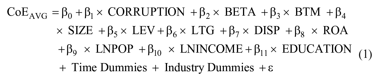
\begin{array}{l} {CoE}_{AVG} = β_{0} + β_{1} \times CORRUPTION + β_{2} \times BETA + β_{3} \times BTM + β_{4} \\ \times SIZE + β_{5} \times LEV + β_{6} \times LTG + β_{7} \times DISP + β_{8} \times ROA \\ + β_{9} \times LNPOP + β_{10} \times LNINCOME + β_{11} \times EDUCATION \\ + Time Dummies + Industry Dummies + ε \end{array}

(1)

The dependent variable in (1) is the implied CoE and the main independent variable of interest is the conviction rate for the state in which the firm is headquartered. The regression model includes controls that are commonly used in the equity pricing literature (Ding et al., 2015; El Ghoul et al., 2012). We control for a firm’s beta (BETA), book-to-market (BTM), size (SIZE), leverage (LEV), long-term growth (LTG), dispersion (DISP), and performance (ROA). In addition, we include state-level controls as our main research variable is at the state level, namely, natural log of population (LNPOP), natural log of gross domestic product (GDP) per capita (LNINCOME), and education attainment (EDUCATION; Jha & Cox, 2015; Smith, 2016). Our independent variables are essentially lagged as they are measured at the end of the previous period. As argued and used in previous studies (Adams et al., 2009; Jiraporn et al., 2009; Kryzanowski & Mohebshahedin, 2016), such a lagged modeling specification helps to alleviate somewhat the concerns associated with endogeneity biases if the exogenous instruments and the shocks chosen to reduce endogeneity concerns are questioned.¹⁴

Sample and Summary Statistics

Our final sample consists of 29,569 firm-year observations for 5,032 firms over the period 1998 to 2017. Our firms cover all 50 U.S. states and Washington, D.C. Our variables are constructed from COMPUTAT, I/B/E/S, and Thomson databases, as well as from the U.S. Census Bureau and Bureau of Economic Analysis. A detailed description of each variable is provided in Appendix A. In reaching our final sample, we ensured that all our variables are available for each firm-year observation. To remove the effects of outliers, all our continuous variables (except for the corruption variables and state-level controls) are winsorized at the 1%/99% level. All regressions control for Fama–French industry and year fixed effects. Standard errors are clustered at the state level.

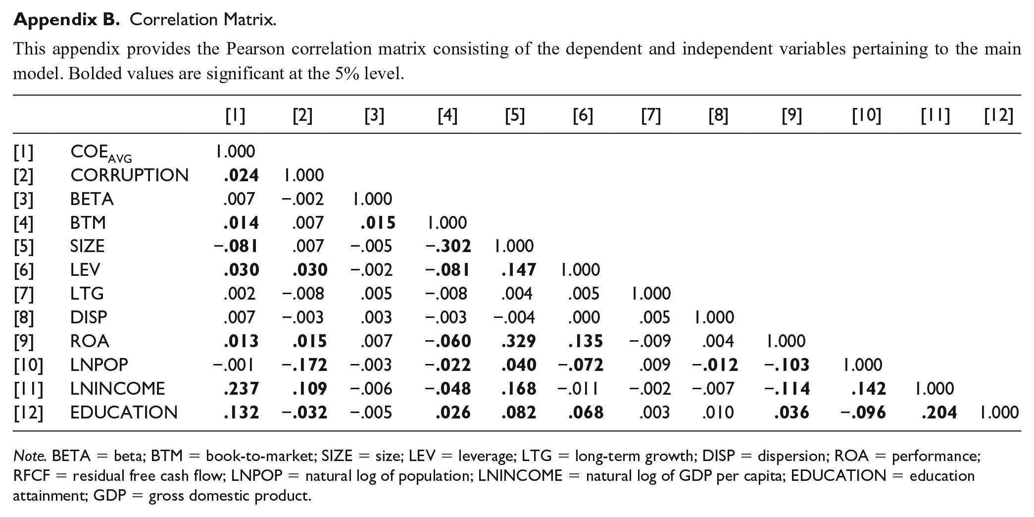
Summary statistics for all variables are provided in columns 1 to 5 of Table 1. The mean (median) corruption rate for our sample period is 0.317 (0.259) per 100,000 people.¹⁵ On average, the CoE (CoE_AVG) is about 6.14% and the mean (median) estimate for the risk factor (β) is slightly above the market beta at 1.225 (1.229). The average firm in our sample is relatively healthy with an ROA of 7.1%, and long-term growth of 16.67%. An average firm also is financially solvent depicted by its low leverage ratio (~18%). The potential for future growth is promising for the sample firms as evidenced by a low average BTM (0.52). We observe no concerning Spearman correlation coefficients between the main variables (Appendix B).

Table 1.

Main Results: Descriptive Statistics.

Variables	(1)M	(2)SD	(3)Q1	(4) Median	(5)Q3	(6)Corruption high	(7)Corruption low	(8)Difference high − low	(9)t statistic for difference
CoE_AVG	6.143	3.008	4.027	5.971	8.148	6.243	6.044	0.199	5.68***
CoE_OJN	7.243	3.550	4.752	7.038	9.605	7.362	7.124	0.237	4.76***
CoE_MPEG	7.279	3.570	4.764	7.085	9.642	7.395	7.163	0.232	7.09***
CoE_CT	5.332	2.611	3.494	5.184	7.074	5.419	5.245	0.174	5.74***
CoE_GLS	4.719	2.314	3.094	4.582	6.252	4.794	4.644	0.150	6.59***
CoE_{AVG_IND}	6.092	1.407	4.831	5.602	7.545	6.210	5.973	0.237	14.53***
CORRUPTION	0.317	0.353	0.183	0.259	0.387	0.465	0.171	0.294	78.76***
CORRUPTION_VEP	0.476	0.489	0.286	0.398	0.581	0.686	0.267	0.419	81.71***
CORRUPTION_VAP	0.423	0.444	0.249	0.342	0.532	0.617	0.230	0.387	83.32***
CORRUPTION_BC	1.059	1.323	0.565	0.876	1.276	1.550	0.570	0.980	68.54***
CORRUPTION_US_SCALE	0.919	0.984	0.574	0.775	1.165	1.309	0.531	0.778	74.01***
BETA	1.225	0.704	0.737	1.229	1.705	1.215	1.235	−0.020	−2.46**
BTM	0.524	0.429	0.220	0.427	0.719	0.539	0.509	0.030	6.02***
SIZE	6.225	1.524	4.993	6.021	7.204	6.230	6.221	0.009	0.49
CASH	0.236	0.252	0.034	0.132	0.372	0.200	0.271	−0.071	−24.38***
LEV	0.178	0.220	0.000	0.089	0.292	0.193	0.164	0.029	11.44***
LTG	16.674	7.848	11.344	16.698	21.987	16.632	16.715	−0.083	−1.91*
DISP	0.134	0.097	0.055	0.116	0.194	0.133	0.135	−0.001	−1.19
ROA	0.071	0.134	0.016	0.087	0.152	0.082	0.061	0.021	13.31***
IO	0.554	0.291	0.313	0.590	0.814	0.548	0.560	−0.012	−3.52***
LNPOP	2.464	0.890	1.834	2.491	3.261	2.374	2.554	−0.180	−17.48***
LNINCOME	10.764	0.239	10.596	10.766	10.929	10.742	10.785	−0.042	−15.36***
EDUCATION	0.788	0.087	0.744	0.804	0.854	0.791	0.785	0.006	5.56***

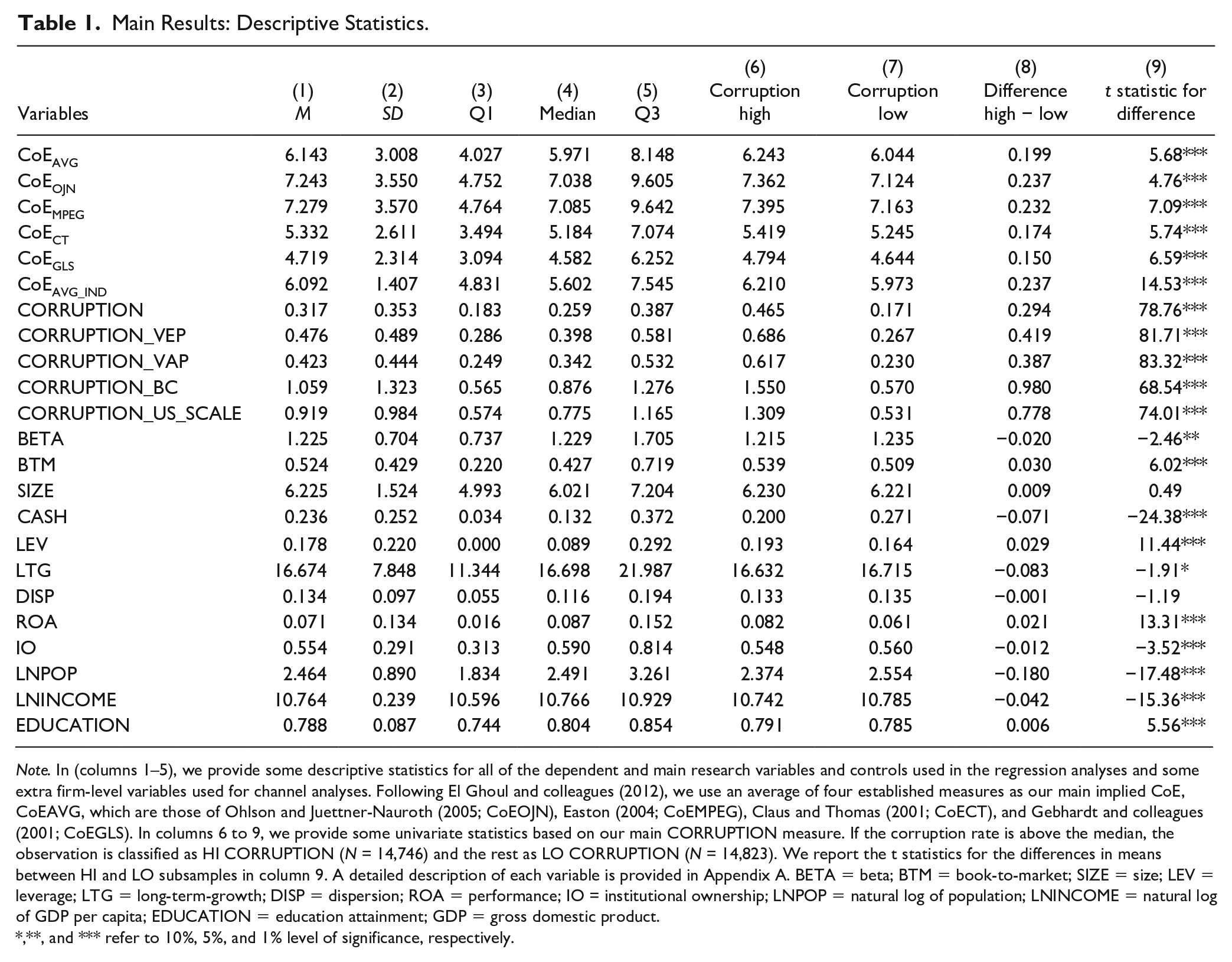
Note. In (columns 1–5), we provide some descriptive statistics for all of the dependent and main research variables and controls used in the regression analyses and some extra firm-level variables used for channel analyses. Following El Ghoul and colleagues (2012), we use an average of four established measures as our main implied CoE, CoEAVG, which are those of Ohlson and Juettner-Nauroth (2005; CoEOJN), Easton (2004; CoEMPEG), Claus and Thomas (2001; CoECT), and Gebhardt and colleagues (2001; CoEGLS). In columns 6 to 9, we provide some univariate statistics based on our main CORRUPTION measure. If the corruption rate is above the median, the observation is classified as HI CORRUPTION (N = 14,746) and the rest as LO CORRUPTION (N = 14,823). We report the t statistics for the differences in means between HI and LO subsamples in column 9. A detailed description of each variable is provided in Appendix A. BETA = beta; BTM = book-to-market; SIZE = size; LEV = leverage; LTG = long-term-growth; DISP = dispersion; ROA = performance; IO = institutional ownership; LNPOP = natural log of population; LNINCOME = natural log of GDP per capita; EDUCATION = education attainment; GDP = gross domestic product.

,**, and *** refer to 10%, 5%, and 1% level of significance, respectively.

Results and Findings

Main Results

We undertake both univariate and multivariate regression analyses to test our hypotheses. The univariate test results for differences in the average values for each variable for the annually classified below (≤ median) and above (>median) medians of states representing low and high state-level corruption rates, respectively, are reported in columns 6 to 9 in Table 1. This is somewhat similar to the method employed by Smith (2016). Most notably, our main CoE measure, CoE_AVG, is higher by about 20 basis points (bps) for firms in the most corrupt versus those in the least corrupt states. Similarly, the components of CoE_AVG, namely, CoE_OJN, CoE_MPEG, CoE_CT, and CoE_GLS, are also higher for firms in high CORRUPTION states.

In Table 2, we present our main regression results with CoE_AVG as the dependent variable. In column 1, we present our baseline model. To mitigate any possible concerns from our sample inclusion of the highly unusual financial crisis period (2008–2009) or highly regulated industries (financial and utilities), we exclude each and rerun our model (column 2 and column 3, respectively). To address any concerns related to our use of a conviction-rate-only–based corruption measure, we rerun our model using three alternate measures of corruption: Butler and colleagues’ type dummy, perception-based rank, and antiethical score (columns 4, 5, and 6, respectively). All regressions control for Fama–French industry and year fixed effects. Standard errors are clustered at the state level. We consistently find statistically significant beta coefficients at the 1% level that imply that CORRUPTION negatively affects CoE, in that, higher corruption results in an increased level of CoE.¹⁶ The relations also carry economic significance. For example, based on the coefficient (0.583) for CORRUPTION in column 1, an increase in the level of corruption that reflects the difference between the fifth least corrupt (Kansas = 0.134) and fifth most corrupt (Mississippi = 0.690) states is associated with a 5.3% increase in a firm’s CoE from the sample mean of 6.143% (Table 1), ceteris paribus. Overall, our findings are consistent with the HCEH. Next, we undertake several robustness checks to ensure that we address possible criticisms of our methodological approach and other econometric concerns.

Table 2.

Main Results: Regression Results.

Variables	(1)Main model	(2)Exclude financial crisis	(3)Exclude financials and utilities	(4)Butler, Fauver, and Mortal dummy approach	(5)Perception-based rank approach	(6)Antiethical score
CORRUPTION	0.583*** (12.21)	0.481*** (7.92)	0.399*** (8.18)	0.184*** (7.57)	0.067*** (11.20)	0.064*** (9.92)
BETA	0.025** (2.14)	0.014 (1.61)	0.015 (1.24)	0.024** (2.18)	0.025** (2.12)	0.022*** (2.62)
BTM	0.023*** (2.58)	0.002 (1.53)	0.008 (1.17)	0.009* (1.92)	0.042* (1.87)	0.049** (1.99)
Size	−0.411*** (−42.46)	−0.080*** (−6.31)	−0.551*** (−5.82)	−0.564*** (−5.73)	−0.332*** (−6.65)	−0.328*** (−9.78)
LEV	0.047*** (2.60)	0.026*** (3.41)	0.044*** (3.53)	0.076* (1.93)	0.083* (1.67)	0.071* (1.92)
LTG	0.010** (2.45)	0.011* (1.66)	0.012* (1.83)	0.021* (1.71)	0.020 (1.57)	0.017 (1.51)
DISP	0.192 (1.20)	0.253 (1.45)	0.120 (1.14)	0.122 (0.71)	0.181 (1.12)	0.161 (1.26)
ROA	0.137** (2.05)	0.199*** (3.10)	0.116*** (2.81)	0.142** (2.35)	0.117* (1.85)	0.123* (1.90)
LNPOP	−0.028** (−2.47)	−0.077*** (−3.86)	−0.030** (−2.45)	−0.020*** (−3.03)	−0.017*** (−3.49)	0.022*** (−3.63)
LNINCOME	0.321*** (30.02)	0.222*** (36.63)	0.304*** (25.48)	0.113*** (10.02)	0.120*** (11.59)	0.103*** (7.67)
EDUCATION	0.240 (1.10)	0.079 (1.34)	0.045 (1.18)	0.010 (1.32)	0.014 (1.56)	0.007 (1.28)
Fixed effects?	Yes	Yes	Yes	Yes	Yes	Yes
Adj. R²	.205	.444	.245	.251	.368	.313
Number of observations	29,569	26,907	24,984	29,569	29,569	29,569

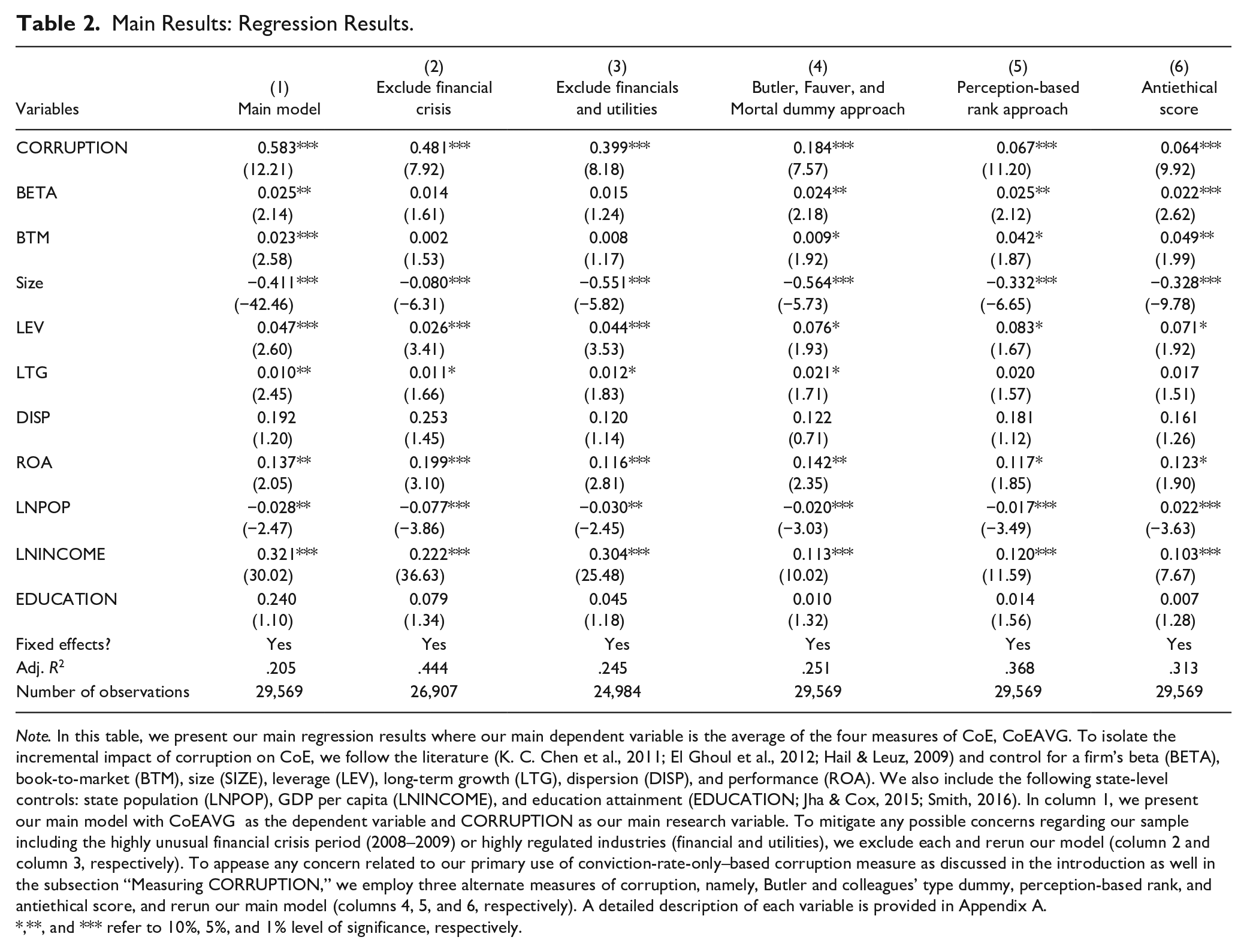
Note. In this table, we present our main regression results where our main dependent variable is the average of the four measures of CoE, CoEAVG. To isolate the incremental impact of corruption on CoE, we follow the literature (K. C. Chen et al., 2011; El Ghoul et al., 2012; Hail & Leuz, 2009) and control for a firm’s beta (BETA), book-to-market (BTM), size (SIZE), leverage (LEV), long-term growth (LTG), dispersion (DISP), and performance (ROA). We also include the following state-level controls: state population (LNPOP), GDP per capita (LNINCOME), and education attainment (EDUCATION; Jha & Cox, 2015; Smith, 2016). In column 1, we present our main model with CoEAVG as the dependent variable and CORRUPTION as our main research variable. To mitigate any possible concerns regarding our sample including the highly unusual financial crisis period (2008–2009) or highly regulated industries (financial and utilities), we exclude each and rerun our model (column 2 and column 3, respectively). To appease any concern related to our primary use of conviction-rate-only–based corruption measure as discussed in the introduction as well in the subsection “Measuring CORRUPTION,” we employ three alternate measures of corruption, namely, Butler and colleagues’ type dummy, perception-based rank, and antiethical score, and rerun our main model (columns 4, 5, and 6, respectively). A detailed description of each variable is provided in Appendix A.

,**, and *** refer to 10%, 5%, and 1% level of significance, respectively.

Additional Robustness Checks

PSM

If firms facing higher CoEs choose to establish HQs in low corruption states, then it may not be corruption that influences CoE as we argue. Instead, it may be firms with a higher propensity to be concerned about CoE that choose to locate in low CORRUPTION states. Furthermore, if the OLS assumption that the covariates and the dependent variable are linearly related is not true, the model could be misspecified. Therefore, we use PSM as described in Rosenbaum and Rubin (1983). We divide our groups into two subgroups based on the median level of CORRUPTION. We consider the group with HI CORRUPTION as the treatment group and those with LO CORRUPTION as the control group. For each of the observations in the treatment and control groups, we calculate the propensity score (i.e., the probability of belonging in the HI CORRUPTION group using a logit model). We use all of our firm-level controls and industry controls as covariates. Then, for each observation from the treated sample, we find the nearest neighbor, the observation from the control group for which the absolute value of the difference in propensity scores is a minimum. We match with replacement. We report the results in Table 3. While the CoE values are significantly different between the two groups, other firm-level variables are not different statistically. Our main findings continue to hold, i.e. CoE is higher by almost 20 bps for firms in the most corrupt states.

Table 3.

Propensity Score Matching.

Variables	Treatment (N = 14,194)HI CORRUPTION			Matched (N = 14,194)LO CORRUPTION			Mean difference	t statistic for M difference
Variables	M	Median	SD	M	Median	SD	Mean difference	t statistic for M difference
CoE_AVG	6.235	6.023	3.113	6.038	5.909	2.895	0.197	5.52***
CoE_OJN	7.353	7.103	3.676	7.117	6.959	3.415	0.236	5.61***
CoE_MPEG	7.386	7.153	3.694	7.156	7.005	3.438	0.230	6.42***
CoE_CT	5.413	5.232	2.703	5.240	5.131	2.512	0.173	4.58***
CoE_GLS	4.789	4.619	2.394	4.639	4.538	2.230	0.149	4.86***
BETA	1.219	1.223	0.701	1.232	1.235	0.703	−0.014	−1.06
BTM	0.535	0.443	0.428	0.520	0.420	0.425	0.014	1.14
SIZE	6.224	6.027	1.522	6.227	6.048	1.532	−0.003	−1.15
LEV	0.188	0.108	0.219	0.169	0.069	0.220	0.019	1.21
LTG	16.634	16.653	7.834	16.714	16.712	7.868	−0.080	−0.86
DISP	0.133	0.115	0.096	0.134	0.115	0.098	−0.001	−0.59
ROA	0.079	0.093	0.129	0.070	0.084	0.134	0.009	1.63

Note. In this table, we report results from the PSM. If firms facing higher CoEs choose to establish HQ in low-corruption states, then corruption may not influence CoE as we argue but instead firms with higher CoE concerns choose to locate in low-CORRUPTION states. We use PSM as described in Rosenbaum and Rubin (1983) to address the possibility of model misspecification if the OLS assumption that the covariates and the dependent variable are linearly related is violated. We divide our groups into two groups based on the median level of CORRUPTION. We consider the group with HI CORRUPTION as the treatment group and those with low CORRUPTION as the control group. For each of the observations in the treatment and control groups, we calculate the propensity score (probability of belonging in the HI CORRUPTION group) using a logit model. We use all of our firm-level controls and industry as covariates. For each observation from the treated sample, we find the nearest neighbor in the control group for which the absolute value of the difference in propensity scores is a minimum. We match with replacement. Whereas the CoE values are significantly different between the two groups, other firm-level variables are not different statistically. Our main findings continue to hold (i.e., CoE is higher by almost 20 bps for firms in the most corrupt states). For all regressions, coefficient estimates and their t statistics (in parentheses) are reported. Regressions control for Fama–French industry and year fixed effects. Standard errors are clustered at the state level. All continuous variables are winsorized at the 1%/99% levels. Definitions of all variables are provided in Appendix A. Coefficients for controls are suppressed for brevity. BETA = beta; BTM = book-to-market; SIZE = size; LEV = leverage; LTG = long-term growth; DISP = dispersion; ROA = performance.

,**, and *** refer to 10%, 5%, and 1% level of significance, respectively.

IV approach

Our analyses thus far assumed that a firm’s selection of headquarter location is exogenously determined. Thus, our OLS estimates potentially may suffer from endogeneity because the level of state corruption may be a determinant of a firm’s choice of headquarter location. This in turn may affect the managerial decision-making processes (Smith, 2016). To address this concern and to obtain purer effects of the corruption measure on CoE, we conduct two two-stage least squares (2SLS) regression analyses.

In the first IV test whose results are reported in columns 1 and 2 of Table 4, we use an instrument similar to that used in other studies with corruption as the main research variable (Nguyen et al., 2018; Smith, 2016). We call the instrument ISOLATION_CAPITAL, whose values theoretically range between zero and one, with zero indicating that no one lives in the capital and one means everyone lives in the capital. The economic intuition is that politicians are likely to be more corrupt in isolated capital cities due to less monitoring from media and electors (Nguyen et al., 2018, p. 25, para 1). In the first-stage regressions, ISOLATION_CAPITAL is directly related to state corruption. Based on the first-stage regression results reported in column 1, the instrument is not weak because the first-stage F stat used to test the null hypothesis that the instrument is weak exceeds the often-used threshold of 10 and the Stock and Yogo (2005) critical values. Another requirement for a valid instrument is that it must satisfy the exclusion criterion (i.e., ISOLATION_CAPITAL must act on CoE only through its relation with state-level corruption). The null that CORRUPTION is exogenous is rejected at a p value of .00.

Table 4.

Instrumental Variable Approach.

Variables	Stage 1DV = CORRUPTION	Stage 2DV = CoE_AVG	Stage 1DV = CORRUPTION	Stage 2DV = CoE_AVG
ISOLATION_CAPITAL	0.428*** (10.90)
CORRUPTION_NEIGHBOR			0.538*** (37.13)
CORRUPTION_IND_AVG			0.868*** (12.82)
CORRUPTION		0.561*** (19.51)		0.427*** (6.22)
Fixed effects?	Yes	Yes	Yes	Yes
Controls?	Yes	Yes	Yes	Yes
Adj. R²	.606	.445	.633	.203
Number of observations	29,569	29,569	29,569	29,569

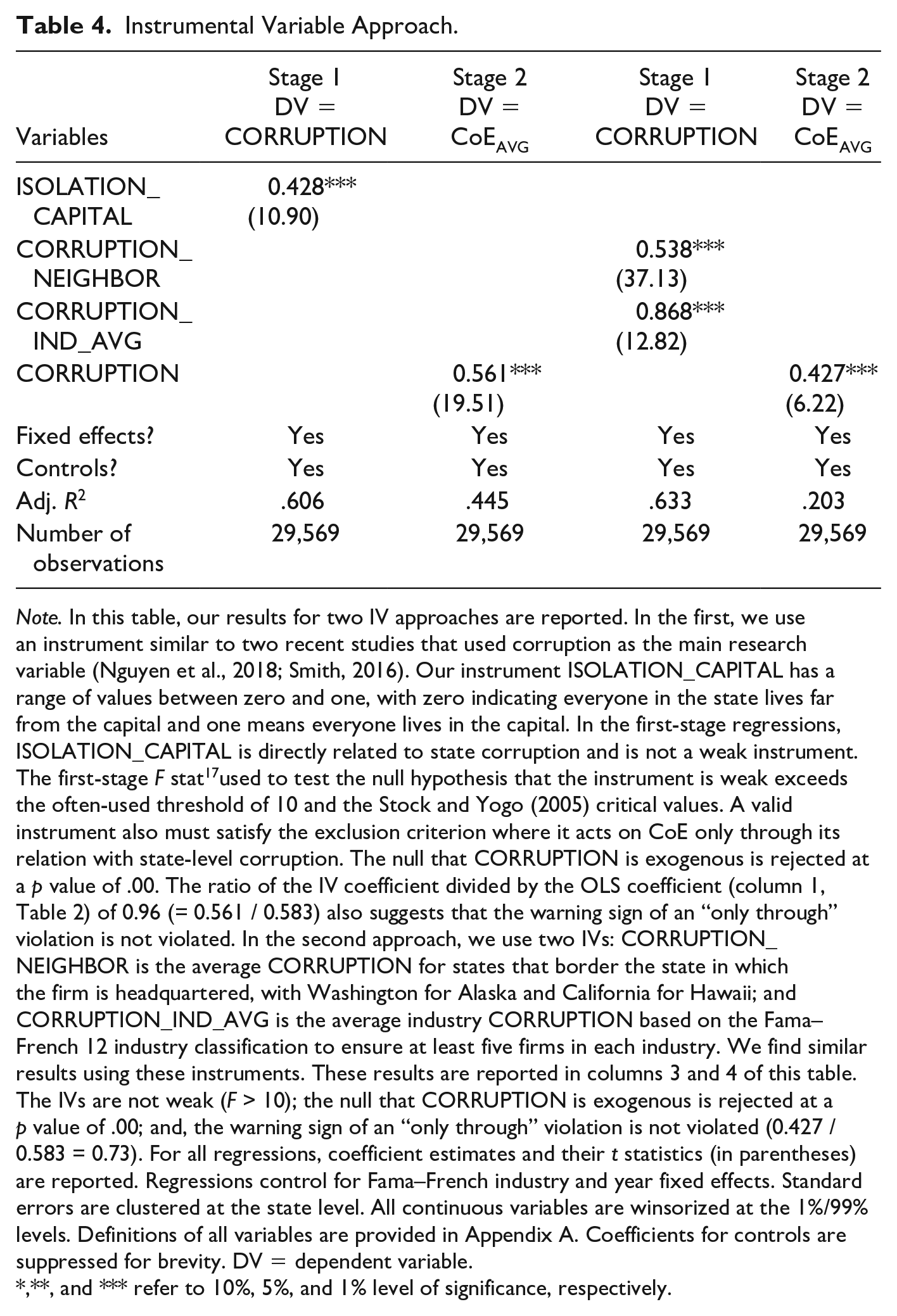
Note. In this table, our results for two IV approaches are reported. In the first, we use an instrument similar to two recent studies that used corruption as the main research variable (Nguyen et al., 2018; Smith, 2016). Our instrument ISOLATION_CAPITAL has a range of values between zero and one, with zero indicating everyone in the state lives far from the capital and one means everyone lives in the capital. In the first-stage regressions, ISOLATION_CAPITAL is directly related to state corruption and is not a weak instrument. The first-stage F stat¹⁷used to test the null hypothesis that the instrument is weak exceeds the often-used threshold of 10 and the Stock and Yogo (2005) critical values. A valid instrument also must satisfy the exclusion criterion where it acts on CoE only through its relation with state-level corruption. The null that CORRUPTION is exogenous is rejected at a p value of .00. The ratio of the IV coefficient divided by the OLS coefficient (column 1, Table 2) of 0.96 (= 0.561 / 0.583) also suggests that the warning sign of an “only through” violation is not violated. In the second approach, we use two IVs: CORRUPTION_NEIGHBOR is the average CORRUPTION for states that border the state in which the firm is headquartered, with Washington for Alaska and California for Hawaii; and CORRUPTION_IND_AVG is the average industry CORRUPTION based on the Fama–French 12 industry classification to ensure at least five firms in each industry. We find similar results using these instruments. These results are reported in columns 3 and 4 of this table. The IVs are not weak (F > 10); the null that CORRUPTION is exogenous is rejected at a p value of .00; and, the warning sign of an “only through” violation is not violated (0.427 / 0.583 = 0.73). For all regressions, coefficient estimates and their t statistics (in parentheses) are reported. Regressions control for Fama–French industry and year fixed effects. Standard errors are clustered at the state level. All continuous variables are winsorized at the 1%/99% levels. Definitions of all variables are provided in Appendix A. Coefficients for controls are suppressed for brevity. DV = dependent variable.

,**, and *** refer to 10%, 5%, and 1% level of significance, respectively.

Based on the second-stage regression results reported in column 2, our main results continue to hold as CORRUPTION continues to result in higher CoE (β = 0.561, t stat = 19.38). As a further indicative test of the “only through” condition, we find that the ratio of the CORRUPTION coefficients from this IV test and the baseline regression is nearly one at 0.96 (= 0.561 / 0.583). Atanasov and Black (2016) note that “A less well known warning sign for an instrument that violates the only through condition is when the IV coefficient estimate is much larger than the OLS estimate” (p. 277) as they and Jiang (2017) find is common in the papers they examine.

It could be argued that political corruption need not be confined to the state where a firm is headquartered but may also include neighboring states. We adapt an IV approach from the social capital literature (Jha & Cox, 2015) to address this concern. We use two IVs in this test. CORRUPTION_NEIGHBOR is the average CORRUPTION for states that border the state in which a firm is headquartered with, Washington for Alaska and California for Hawaii; and CORRUPTION_IND_AVG is the average industry CORRUPTION based on the Fama–French 12 industry classification to ensure that at least five firms are available in each industry. The results reported in columns 3 and 4 of Table 4 are consistent with previous results. The IVs are not weak (F > 10), the null that CORRUPTION is exogenous is rejected at a p value of .00, and that the warning sign of an “only through” violation is not violated (ratio of the CORRUPTION coefficients from this IV test and the baseline regression of 0.427 / 0.583 = 0.73).

Tests to explore channels

Financial constraints, agency issues, and external firm monitoring are important factors considered by investors in assessing a firm’s riskiness when determining the firm’s CoE. We use leverage (LEV), residual free cash flow (RFCF), and institutional ownership (IO), respectively, to measure each factor. The detailed discussion to justify these choices was provided in the introduction section of this article.¹⁸

Table 5 reports the results when we test the mediation effect on CORRUPTION of three channel variables using dummy variables where HI indicates a value of one (0 otherwise) for above median leverage (LEV), RFCF, and IO. Consistent results are reported for the subsamples in OSA, Table A.4.

Table 5.

Tests of Mediation Effect of Three Channel Variables.

	(1)DUMMY = LO LEV	(2)DUMMY = HI RFCF	(3)DUMMY = LO IO
CORRUPTION	0.170* (1.83)	0.234** (2.15)	0.472*** (3.12)
CORRUPTION × DUMMY	0.304*** (3.38)	0.289*** (8.33)	0.125*** (2.76)
DUMMY	−0.029* (−1.69)	−0.011* (−1.82)	−0.047** (−2.36)
Fixed effects?	Yes	Yes	Yes
Controls?	Yes	Yes	Yes
Adj. R²	.205	.206	.201
Number of observations	29,569	29,569	29,569

Note. This table reports the results when we test the mediation effect on CORRUPTION of three channel variables using dummy variables where HI indicates a value of one (0 otherwise) for above median leverage (LEV), residual free cash flow (RFCF), and institutional ownership (IO). The reported results for these three channels show that the effects of corruption on CoE are significantly higher for firms with lower leverage, higher levels of RFCF, and lower levels of IO. Consistent results are reported for the subsamples in OSA, Table A.4. For all regressions, coefficient estimates and their t statistics (in parentheses) are reported. Regressions control for Fama–French industry and year fixed effects. Standard errors are clustered at the state level. All continuous variables are winsorized at the 1%/99% levels. Definitions of all variables are provided in Appendix A. Coefficients for controls are suppressed for brevity.

,**, and *** refer to 10%, 5%, and 1% level of significance, respectively.

The results reported in Table 5 for these three channels show that the effects of corruption on CoE are significantly higher for firms with lower leverage, higher levels of RFCF, and lower levels of IO. The results for the RFCF and IO channels are as expected, and the results for the LEV channel extend the findings of Smith (2016) by providing some initial evidence that the net benefits from corruption shielding using leverage are positive.

Additional variables

Because most firms located in a state may belong to similar industries, the effect of industry should be better controlled for to capture the true effect of state-level political corruption. Based on the suggestion from an anonymous referee, we add the industry median CoE (CoE_{AVG_IND}) to the baseline regression. The industry classifications are based on the Fama–French 12 industry codes, which are equivalent to a two-digit SIC classification. These results are presented in Table 6, column 1. Although the estimated coefficient for CoE_{AVG_IND} is positive and highly significant as expected, there is little change in the magnitude and significance of the estimated coefficient for CORRUPTION from its baseline counterpart.

Table 6.

Additional Variables.

Variables	(1)	(2)	(3)	(4)	(5)	(6)	(7)
CORRUPTION	0.578*** (12.15)	0.588*** (12.29)	0.450*** (16.75)	0.583*** (12.20)	0.549*** (11.24)	0.581*** (12.22)	0.594*** (11.30)
INDUSTRY MEDIAN CoE	0.661*** (13.47)
STATE CAP HQ (dummy)		0.085* (1.66)	0.032* (1.69)
CORRUPTION × STATE CAP HQ (dummy)			0.130** (2.06)
KLD GOV STRENGTH				−0.027* (−1.87)
KLD GOV SCORE					−0.025* (−1.81)
KLD STRONG GOV (dummy)						−0.018* (−1.80)	−0.000(−0.88)
CORRUPTION × KLD STRONG GOV (dummy)							−0.055** (−2.49)
Fixed effects?	Yes	Yes	Yes	Yes	Yes	Yes	Yes
Controls?	Yes	Yes	Yes	Yes	Yes	Yes	Yes
Adj. R²	.211	.205	.209	.205	.205	.205	.205
Number of observations	29,569	29,569	29,569	23,904	23,904	23,904	23,904

Note. In this table, the effect of CORRUPTION on CoE is examined when each of the following covariates is added to the baseline regression: the industry median CoE (CoE_{AVG_IND}) in column 1 based on Fama–French 12 industry classification to ensure at least five firms in each industry; a STATE CAP HQ dummy variable in column 2 equal to one if a firm is headquartered in a state capital and zero otherwise; the KLD governance strength and net (i.e., strengths − concerns) scores in columns 3 and 4, respectively; and CORRUPTION_NEIGHBOR which is the average CORRUPTION for states that border the state in which a firm is headquartered in column 5, with Washington for Alaska and California for Hawaii. In all cases, our results continue to hold. For all regressions, coefficient estimates and their t statistics (in parentheses) are reported. Regressions control for Fama–French industry and year fixed effects. Standard errors are clustered at the state level. All continuous variables are winsorized at the 1%/99% levels. Definitions of all variables are provided in Appendix A. Coefficients for controls are suppressed for brevity.

,**, and *** refer to 10%, 5%, and 1% level of significance, respectively.

Because the within-state location of a firm may also be important, we examine the effect on the baseline CORRUPTION–CoE relation of whether a firm is headquartered in the state capital or not. For this test, we augment our baseline regression with a STATE CAP HQ dummy variable equal to one if a firm is headquartered in a state capital and zero otherwise. The results for adding this dummy variable are reported in Table 6, columns 2 and 3. The estimated coefficient for this dummy variable and CORRUPTION are both positive and significant. The estimated coefficient for CORRUPTION × STATE CAP HQ is positive and significant, which implies that firms headquartered in a state capital have significantly higher CoE.¹⁹

Although we use IO as a proxy for (external) corporate governance, it could be argued that internal measures of corporate governance also should be used. Based on the suggestion from an anonymous referee, we examine the effect on CORRUPTION when two internal governance covariates are added to the baseline regression. The results for adding the KLD governance strength and net (i.e., strengths − concerns) scores are reported in Table 6, columns 4 and 5, respectively. All results are as expected. The estimated coefficient for CORRUPTION is positive and significant, CoE is significantly and negatively related to both governance measures, and the negative effect of CORRUPTION on CoE is still significant but weaker with stronger governance (column 7).

Quasi-experiments using two shocks

We use two quasi-natural experiments that were shocks to the environment for political corruption to further deal with endogeneity and to further support a causal interpretation of our results: namely, the MF Campaign Reform Act of 2003, which was one of the strongest legislations against soft-money-in-politics; and its weakening by the 2010 Citizen United v. Federal Election Commission decision by the SCOTUS. As in Dyck and colleagues (2019) for the Deep-Water Horizon shock, we use a DiD approach using 2001 to 2002 and 2008 to 2009 as the PRE-SHOCK periods for MF and SCOTUS, respectively, and 2003 to 2004 and 2010 to 2011 as the POST-SHOCK periods for MF and SCOTUS, respectively. We also collapse the 2-year pre- and post-event periods each into one observation to address serial correlation (Bertrand et al., 2004). We classify the firms preshock that have made above-median political contributions as being treated. These results are presented in Table 7. We designate the top 10 industry contributors between 1980 and 1996 as HI CONTRIBUTOR industries. These industries accounted for more than 90% of total nonindividual soft money contributions during this period, which precedes our sample period. This is the common approach for determining the treatment effect (Dyck et al., 2019).

Table 7.

Quasi-Experiment Tests Using Two Shocks.

	SHOCK = MF2001–2004	SHOCK = SCOTUS2009–2012
CORRUPTION	0.152** (2.03)	0.722*** (4.09)
HI CONTRIBUTOR	−0.058(−0.42)	−0.429** (−2.03)
POST-SHOCK	−0.011(−0.10)	−0.013(−0.11)
CORRUPTION × HI CONTRIBUTOR × POST-SHOCK	−0.224* (−1.77)	0.477* (1.65)
Other controls and other interactions?	Yes	Yes
Observations	6,281	5,320
Adjusted R²	.107	.123

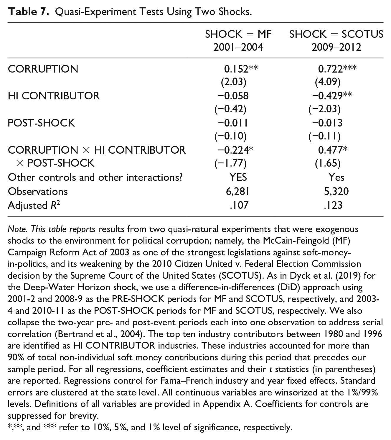
Note. This table reports results from two quasi-natural experiments that were exogenous shocks to the environment for political corruption; namely, the McCain-Feingold (MF) Campaign Reform Act of 2003 as one of the strongest legislations against soft-money-in-politics, and its weakening by the 2010 Citizen United v. Federal Election Commission decision by the Supreme Court of the United States (SCOTUS). As in Dyck et al. (2019) for the Deep-Water Horizon shock, we use a difference-in-differences (DiD) approach using 2001-2 and 2008-9 as the PRE-SHOCK periods for MF and SCOTUS, respectively, and 2003-4 and 2010-11 as the POST-SHOCK periods for MF and SCOTUS, respectively. We also collapse the two-year pre- and post-event periods each into one observation to address serial correlation (Bertrand et al., 2004). The top ten industry contributors between 1980 and 1996 are identified as HI CONTRIBUTOR industries. These industries accounted for more than 90% of total non-individual soft money contributions during this period that precedes our sample period. For all regressions, coefficient estimates and their t statistics (in parentheses) are reported. Regressions control for Fama–French industry and year fixed effects. Standard errors are clustered at the state level. All continuous variables are winsorized at the 1%/99% levels. Definitions of all variables are provided in Appendix A. Coefficients for controls are suppressed for brevity.

,**, and *** refer to 10%, 5%, and 1% level of significance, respectively.

As in Dyck and colleagues (2019), our coefficient of interest is the triple interaction coefficient for CORRUPTION × HI CONTRIBUTOR × POST-SHOCK that captures the differential effect of HI CONTRIBUTOR for treated firms relative to control firms after the shock. As expected, we find that the coefficients for the triple interaction variable designed to capture the differential effect for treated firms relative to control firms after the shock are significant and negative for the MF shock and significant and positive for the SCOTUS shock (Table 7).

Discussion of Results

As discussed in the earlier sections of this article, an important concern is if the relation we capture between a politically corrupt environment and CoE is indeed real or just a spurious correlation. In view of the robustness tests undertaken, we believe that it is highly unlikely that what we find is spurious in nature. To reemphasize, the “higher CORRUPTION leads to higher CoE” relationship continues to hold when we use PSM (Table 3), or the IV approach (Table 4), or the DiD approach using exogenous shocks from two quasi-natural experiments to further support causation inferences (Table 7) or alternate proxies for CORRUPTION (columns 4–6, Table 2), or alternate measurement methods for CORRUPTION (OSA, Table A.2). Finally, these results are robust to various other robustness checks, namely, excluding regulated industries and excluding the financial crisis period. Overall, these results are consistent with the HCEH.

Concluding Remarks

A common belief among the general population is that corruption is bad morally and economically and should, therefore, be restricted by law. However, political corruption continues to exist in the United States as a form of rent seeking or more indirectly through political connections or quid pro quo campaign contributions. Our investigation fills a gap in this literature by being the first to examine how political corruption affects CoE due to the importance of CoE in firm valuation and in setting corporate financing, investment, and capital structure policies. Our study can be extended by examining the effect of the relation between CoE and CORRUPTION by examining how it is affected by the location of the firm’s suppliers and customers, and by the characteristics of its labor force and unionization.

Our study has a strong connection with the literature that links a firm’s social performance with its financial performance (review article of Servaes & Tamayo, 2017). Studies have shown that social performance (proxied by CSR scores) is associated with financial performance in the form of a lower CoE (Dhaliwal et al., 2011, lower cost of debt (Goss & Roberts, 2011), better postmerger returns (Deng et al., 2013), lower firm-level risk (Bouslah et al., 2013), better reputation (Brammer & Millington, 2005), and better future performance (Van Beurden & Gössling, 2008). However, there is a lack of consensus within the literature that investigates the social performance–financial performance relationship (Baron et al., 2011; Margolis & Walsh, 2003; Mattingly & Berman, 2006; Orlitzky et al., 2003). From a financial point of view, political corruption as a form of social performance dealing with ethical behavior can affect financial performance or value or CoE if and only if it affects expected future cash flows and/or risk at the firm level. Shielding against political corruption also is somewhat related to greenwashing, which is a marketing or communication strategy whose aim is to hide the most controversial aspects related to corporate sustainability (Seele & Gatti, 2017). Forms of greenwashing (i.e., attention deflection and decoupling) and deceptive manipulation (Siano et al., 2017) consist of corporate identity-washing practices designed to reap the benefits of a “green” image without taking any material actions to be green. We contribute to the social performance–financial performance literature by showing that political corruption by adversely affecting a firm’s future risk and/or cash flows from firm shielding leads to a higher firm CoE.

There is a body of literature in business and society that explores the influence of a firm’s geographic location on its social performance (e.g., CSR activities). Husted and colleagues (2016) find that CSR engagement reduces a firm’s CoE and the effect is strengthened in places where neighboring firms are more CSR active. Jha and Cox (2015) report that firms located in highly trusted areas with dense networks (high social capital) produce better social performance (proxied by CSR). Hossain and Kryzanowski (2020) show that political corruption is negatively associated with a firm’s social performance. Then, there are studies that show a link between a firm’s location and its CoE. For example, El Ghoul and colleagues (2012) find that firms located in more religious areas enjoy lower CoE. Gupta and colleagues (2018) find that firms situated in areas of high trust and dense networks (high social capital) enjoy lower CoE. Other studies find that the level of corporate misbehavior varies across geographic regions (Parsons et al., 2018) and firms forum shop for court hearings of, for example, patent litigations (Cohen et al., 2019).²⁰ In summary, these studies show that geographic location has a significant influence on a firm’s social performance as well as its financial performance that is positive for firms located in geographic locations with more trust (alternatively less political corruption), and that geographic location is a mechanism for shielding against corruption or litigation that has consequences for firm value.

Supplemental Material

BAS-19-0259R2_OSA_20191201-formatted – Supplemental material for Political Corruption and Cost of Equity

Supplemental material, BAS-19-0259R2_OSA_20191201-formatted for Political Corruption and Cost of Equity by Ashrafee Tanvir Hossain and Lawrence Kryzanowski in Business & Society

Footnotes

Appendix

Appendix B.

Correlation Matrix.

This appendix provides the Pearson correlation matrix consisting of the dependent and independent variables pertaining to the main model. Bolded values are significant at the 5% level.

		[1]	[2]	[3]	[4]	[5]	[6]	[7]	[8]	[9]	[10]	[11]	[12]
[1]	COE_AVG	1.000
[2]	CORRUPTION	.024	1.000
[3]	BETA	.007	−.002	1.000
[4]	BTM	.014	.007	.015	1.000
[5]	SIZE	−.081	.007	−.005	−.302	1.000
[6]	LEV	.030	.030	−.002	−.081	.147	1.000
[7]	LTG	.002	−.008	.005	−.008	.004	.005	1.000
[8]	DISP	.007	−.003	.003	−.003	−.004	.000	.005	1.000
[9]	ROA	.013	.015	.007	−.060	.329	.135	−.009	.004	1.000
[10]	LNPOP	−.001	−.172	−.003	−.022	.040	−.072	.009	−.012	−.103	1.000
[11]	LNINCOME	.237	.109	−.006	−.048	.168	−.011	−.002	−.007	−.114	.142	1.000
[12]	EDUCATION	.132	−.032	−.005	.026	.082	.068	.003	.010	.036	−.096	.204	1.000

Note. BETA = beta; BTM = book-to-market; SIZE = size; LEV = leverage; LTG = long-term growth; DISP = dispersion; ROA = performance; RFCF = residual free cash flow; LNPOP = natural log of population; LNINCOME = natural log of GDP per capita; EDUCATION = education attainment; GDP = gross domestic product.

Acknowledgements

We thank Stephen Pavelin (associate editor) and three anonymous referees for their valuable comments and suggestions. Hossain thanks Memorial University of Newfoundland for providing financial support for this project. Kryzanowski thanks the Senior Concordia University Research Chair in Finance and the Social Sciences and Humanities Research Council of Canada (SSHRC, Grant 435-2018-048) for providing financial support. All remaining errors are our own.

Declaration of Conflicting Interests

The authors declared no potential conflicts of interest with respect to the research, authorship, and/or publication of this article.

Funding

The authors disclosed receipt of the following financial support for the research, authorship, and/or publication of this article: The Memorial University of Newfoundland and the Senior Concordia University Research Chair in Finance and the Social Sciences and Humanities Research Council of Canada (SSHRC, Grant 435-2018-048) provided financial support for this project.

ORCID iD

Lawrence Kryzanowski

Supplemental Material

Supplemental material for this article is available online.

Notes

Author Biographies

Ashrafee Tanvir Hossain, PhD, CFA, is an associate professor at the Faculty of Business Administration at the Memorial University of Newfoundland. His research interests include corporate finance, corporate governance, financial regulations, mergers and acquisitions, corporate social responsibility, and sustainability. His articles have been accepted/published in such journals as Accounting & Finance, Business & Society, Journal of Financial Research, Journal of Management & Governance.

Lawrence Kryzanowski (PhD, University of British Columbia) is professor and Senior Concordia University Research Chair in Finance in the Molson School of Business. His research interests focus on corporate structure, governance and firm strategic choices; and effect of natural disasters, social considerations, and political corruption, uncertainty, and monetary initiatives on corporate and investor decisions. His articles have appeared in such journals as Bell (Rand) Journal of Economics, Journal of Banking & Finance, Journal of Business Ethics, Journal of Corporate Finance, Journal of Economic Dynamics and Control, Journal of Finance, Journal of Financial & Quantitative Analysis, Journal of Financial Economics, Journal of Financial Intermediation, Journal of Financial Markets, Journal of Money, Credit and Banking, and Journal of Urban Economics.

References

Abel

A. B.

(1999). Risk premia and term premia in general equilibrium. Journal of Monetary Economics, 43, 3–33.

Adams

J. C.

Mansi

S. A.

Nishikawa

(2009). Internal governance mechanisms and operational performance: Evidence from index mutual funds. Review of Financial Studies, 23, 1261–1286.

Agrawal

Knoeber

C. R.

(2001). Do some outside directors play a political role? The Journal of Law and Economics, 44(1), 179–198.

Aidt

T. S.

(2003). Economic analysis of corruption: A survey. The Economic Journal, 113(491), F632–F652.

Aidt

T. S.

(2009). Corruption, institutions, and economic development. Oxford Review of Economic Policy, 25(2), 271–291.

Albuquerue

Wang

(2008). Agency conflicts, investment, and asset pricing. The Journal of Finance, 63(1), 1–40.

Atanasov

Black

(2016). Shock-based causal inference in corporate finance and accounting research. Critical Finance Review, 5, 207–304.

Attig

Boubakri

El Ghoul

Guedhami

(2016). The global financial crisis, family control, and dividend policy. Financial Management, 45(2), 291–313.

Attig

Cleary

El Ghoul

Guedhami

(2013). Institutional investment horizons and the cost of equity capital. Financial Management, 42(2), 441–477.

10.

Attig

Guedhami

Mishra

(2008). Multiple large shareholders, control contests, and implied cost of equity. Journal of Corporate Finance, 14(5), 721–737.

11.

Baron

D. P.

Harjoto

M. A.

(2011). The economics and politics of corporate social performance. Business and Politics, 13(2), 1–46.

12.

Barry

C. B.

Brown

S. J.

(1985). Differential information and security market equilibrium. Journal of Financial and Quantitative Analysis, 20(4), 407–422.

13.

Bertrand

Duflo

Mullainathan

(2004). How much should we trust differences-in-differences estimates? The Quarterly Journal of Economics, 119(1), 249–275.

14.

Borisov

Goldman

Gupta

(2016). The corporate value of (corrupt) lobbying. Review of Financial Studies, 29(4), 1039–1071.

15.

Botosan

C. A.

Plumlee

M. A.

Xie

(2004). The role of information precision in determining the cost of equity capital. Review of Accounting Studies, 9(2–3), 233–259.

16.

Boubakri

Guedhami

Mishra

(2010). Family control and the implied cost of equity: Evidence before and after the Asian financial crisis. Journal of International Business Studies, 41(3), 451–474.

17.

Boubakri

Guedhami

Mishra

Saffar

(2012). Political connections and the cost of equity capital. Journal of Corporate Finance, 18(3), 541–559.

18.

Boubakri

Mansi

S. A.

Saffar

(2013). Political institutions, connectedness, and corporate risk-taking. Journal of International Business Studies, 44(3), 195–215.

19.

Bouslah

Kryzanowski

M’Zali

(2013). The impact of the dimensions of social performance on firm risk. Journal of Banking & Finance, 37, 1258–1273.

20.

Boylan

R. T.

Long

C. X.

(2003). Measuring public corruption in the American states: A survey of state house reporters. State Politics and Policy Quarterly, 3(4), 420–438.

21.

Brammer

Millington

(2005). Corporate reputation and philanthropy: An empirical analysis. Journal of Business Ethics, 61(1), 29–44.

22.

Brown

N. C.

Smith

J. D.

White

R. M.

Zutter

C. J.

(2018, March 22). Political corruption and firm value in the U.S. https://ssrn.com/abstract=3147385

23.

Buchanan

J. M.

Tullock

(1962). The calculus of consent: Logical foundations of constitutional democracy [Ann Arbor paperbacks]. Liberty Fund Inc.

24.

Bushee

B. J.

(1998). The influence of institutional investors on myopic R&D investment behavior. Accounting Review, 73(3), 305–333.

25.

Butler

A. W.

Fauver

Mortal

(2009). Corruption, political connections, and municipal finance. The Review of Financial Studies, 22(7), 2873–2905.

26.

Campante

F. R.

Q. A.

(2014). Isolated capital cities, accountability, and corruption: Evidence from US states. American Economic Review, 104(8), 2456–2481.

27.

Caprio

Faccio

McConnell

(2013). Sheltering corporate assets from political extraction. Journal of Law, Economics, and Organization, 29(2), 332–354.

28.

Chen

C. J.

Ding

Kim

C. F.

(2010). High-level politically connected firms, corruption, and analyst forecast accuracy around the world. Journal of International Business Studies, 41(9), 1505–1524.

29.

Chen

K. C.

Chen

Wei

K. J.

(2009). Legal protection of investors, corporate governance, and the cost of equity capital. Journal of Corporate Finance, 15(3), 273–289.

30.

Chen

K. C.

Chen

Wei

K. J.

(2011). Agency costs of free cash flow and the effect of shareholder rights on the implied cost of equity capital. Journal of Financial and Quantitative Analysis, 46(1), 171–207.

31.

Chen

Harford

(2007). Monitoring: Which institutions matter? Journal of Financial Economics, 86(2), 279–305.

32.

Citizens United, Appellant v. Federal Election Commission. 558 U.S. 310 (more) 130 S. Ct. 876; 175 L. Ed. 2d 753; 2010 U.S. LEXIS 766

33.

Claessens

Feijen

Laeven

(2008). Political connections and preferential access to finance: The role of campaign contributions. Journal of Financial Economics, 88(3), 554–580.

34.

Claus

Thomas

(2001). Equity premia as low as three percent? Evidence from analysts’ earnings forecasts for domestic and international stock markets. The Journal of Finance, 56(5), 1629–1666.

35.

Cochrane

J. H.

(1997). Where is the market going? Uncertain facts and novel theories. Economic Perspectives, XXI, 3–37.

36.

Cohen

Gurun

U. G.

Kominers

S. D.

(2019). Patent trolls: Evidence from targeted firms. Management Science, 65(12), 5461–5486.

37.

Coles

J. L.

Loewenstein

Suay

(1995). On equilibrium pricing under parameter uncertainty. Journal of Financial and Quantitative Analysis, 30(3), 347–364.

38.

Cooper

M. J.

Gulen

Ovtchinnikov

A. V.

(2010). Corporate political contributions and stock returns. The Journal of Finance, 65(2), 687–724.

39.

Cull

L. C.

(2005). Institutions, ownership, and finance: The determinants of profit reinvestment among Chinese firms. Journal of Financial Economics, 77(1), 117–146.

40.

Damodaran

(1994). Damodaran on valuation: Security analysis for investment and corporate finance. Wiley.

41.

Dass

Nanda

Xiao

S. C.

(2016). Public corruption in the United States: Implications for local firms. Review of Corporate Financial Studies, 5(1), 102–138.

42.

Dass

Nanda

V. K.

Xiao

S. C.

(2018). Geographic clustering of corruption in the US [Working paper]. https://papers.ssrn.com/sol3/papers.cfm?abstract_id=2981317

43.

Davis

White

K. R.

(2018, July 16). Is justice blind? Evidence from Federal corruption convictions. https://ssrn.com/abstract=3214973 or https://dx-doi-org.web.bisu.edu.cn/10.2139/ssrn.3214973

44.

Deng

Kang

J. K.

Low

B. S.

(2013). Corporate social responsibility and stakeholder value maximization: Evidence from mergers. Journal of Financial Economics, 110(1), 87–109.

45.

Dhaliwal

D. S.

O. Z.

Tsang

Yang

Y. G.

(2011). Voluntary nonfinancial disclosure and the cost of equity capital: The initiation of corporate social responsibility reporting. The Accounting Review, 86(1), 59–100.

46.

Ding

X. S.

Rahman

Saadi

(2015). Housing price growth and the cost of equity capital. Journal of Banking & Finance, 61, 283–300.

47.

Duchin

Sosyura

(2012). The politics of government investment. Journal of Financial Economics, 106(1), 24–48.

48.

Durnev

Fauver

(2011). Stealing from thieves: Expropriation risk, firm governance and performance [CEI working paper]. https://papers.ssrn.com/sol3/papers.cfm?abstract_id=970969

49.

Dyck

Lins

K. V.

Roth

Wagner

H. F.

(2019). Do institutional investors drive corporate social responsibility? International evidence. Journal of Financial Economics, 131(3), 693–714.

50.

El Ghoul

Guedhami

Kwok

C. C.

Mishra

D. R.

(2011). Does corporate social responsibility affect the cost of capital? Journal of Banking & Finance, 35(9), 2388–2406.

51.

El Ghoul

Guedhami

Pittman

Saadi

(2012). Does religion matter to equity pricing? Journal of Business Ethics, 111(4), 491–518.

52.

Faccio

(2003). Politically-connected firms: Can they squeeze the state? [SSRN working paper]. https://papers.ssrn.com/sol3/papers.cfm?abstract_id=305099

53.

Faccio

(2006). Politically connected firms. American Economic Review, 96(1), 369–386.

54.

Faccio

(2010). Differences between politically connected and non-connected firms: A cross-country analysis. Financial Management, 39(3), 905–928.

55.

Faccio

Masulis

McConnell

(2006). Political connections and corporate bailouts. Journal of Finance, 61(6), 2597–2635.

56.

Fama

E. F.

Jensen

M. C.

(1983). Agency problems and residual claims. The Journal of Law and Economics, 26(2), 327–349.

57.

Fisman

(2001). Estimating the value of political connections. American Economic Review, 91(4), 1095–1102.

58.

Francis

B. B.

Hasan

Sun

(2016). CEO political preference and corporate tax sheltering. Journal of Corporate Finance, 38, 37–53.

59.

Garner

B. A.

Black

H. C.

(2004). Black’s Law dictionary. Thomson/West.

60.

Gebhardt

W. R.

Lee

C. M.

Swaminathan

(2001). Toward an implied cost of capital. Journal of Accounting Research, 39(1), 135–176.

61.

Glaeser

E. L.

Saks

R. E.

(2006). Corruption in America. Journal of Public Economics, 90, 1053–1072.

62.

Gode

Mohanram

(2003). Inferring the cost of capital using the Ohlson–Juettner model. Review of Accounting Studies, 8(4), 399–431.

63.

Goldman

Rocholl

(2009). Do politically connected boards affect firm value? Review of Financial Studies, 22(6), 2331–2360.

64.

Goldman

Rocholl

(2013). Politically connected boards of directors and the allocation of procurement contracts. Review of Finance, 17(5), 1617–1648.

65.

Gordon

J. R.

Gordon

M. J.

(1997). The finite horizon expected return model. Financial Analysts Journal, 53, 52–61.

66.

Gordon

M. J.

(1963). Optimal investment and financing policy. The Journal of Finance, 18(2), 264–272.

67.

Goss

Roberts

G. S.

(2011). The impact of corporate social responsibility on the cost of bank loans. Journal of Banking & Finance, 35(7), 1794–1810.

68.

Gounopoulos

Huang

(2017, June 13–15, 2018). Political corruption and firm access to the initial public offering market [Conference session]. In FMA European Conference, Kristiansand, Norway.

69.

Guedhami

Mishra

(2009). Excess control, corporate governance and implied cost of equity: International evidence. Financial Review, 44(4), 489–524.

70.

Gupta

Raman

Shang

(2018). Social capital and the cost of equity. Journal of Banking & Finance, 87, 102–117.

71.

Hail

Leuz

(2009). Cost of capital effects and changes in growth expectations around US cross-listings. Journal of Financial Economics, 93(3), 428–454.

72.

Hossain

A. T.

Kryzanowski

(2020). Political corruption and corporate social responsibility (CSR) [Working paper].

73.

Hossain

A. T.

Kryzanowski

X. B.

(2020). US political corruption and loan pricing. Journal of Financial Research. https://doi.org/10.1111/jfir.12217

74.

Houston

J. F.

Jiang

L. L.

Lin

(2014). Political connections and the cost of bank loans. Journal of Accounting Research, 52(1), 193–243.

75.

Husted

B. W.

Jamali

Saffar

(2016). Near and dear? The role of location in CSR engagement. Strategic Management Journal, 37(10), 2050–2070.

76.

Ibbotson Associates, Inc. (1996). Cost of capital quarterly.

77.

Jensen

M. C.

(1986). Agency costs of free cash flow, corporate finance, and takeovers. The American Economic Review, 76(2), 323–329.

78.

Jha

Chen

(2015). Audit fees and social capital. The Accounting Review, 90(2), 611–639.

79.

Jha

Cox

(2015). Corporate social responsibility and social capital. Journal of Banking & Finance, 60, 252–270.

80.

Jiang

(2017). Have instrumental variables brought us closer to the truth. The Review of Corporate Finance Studies, 6(2), 127–140.

81.

Jiraporn

Singh

Lee

C. I.

(2009). Ineffective corporate governance: Director busyness and board committee memberships. Journal of Banking & Finance, 33, 819–828.

82.

Joh

S. W.

Chiu

M. M.

(2004, August). Loans to distressed firms: Political connections, related lending, business group affiliation and bank governance. In Econometric Society 2004 Far Eastern Meetings (No. 790). Econometric Society. https://ideas.repec.org/p/ecm/feam04/790.html

83.

Johnson

Mitton

(2003). Cronyism and capital controls: Evidence from Malaysia. Journal of Financial Economics, 67(2), 351–382.

84.

Kaplan

Zingales

(1997). Do investment-cash flow sensitivities provide useful measures of financing constraints? Quarterly Journal of Economics, 112(1), 169–215.

85.

Khwaja

A. I.

Mian

(2005). Do lenders favor politically connected firms? Rent provision in an emerging financial market. Quarterly Journal of Economics, 120(4), 1371–1411.

86.

Kocherlakota

N. R.

(1996). The equity premium: It’s still a puzzle. Journal of Economic Literature, 34(1), 42–71.

87.

Kryzanowski

Mohebshahedin

(2016). Board governance, monetary interest and closed-end fund performance. Journal of Corporate Finance, 38, 196–217.

88.

Kusnetz

(2015, November 19). Secrecy, corruption and conflicts of interest pervade state governments. USA Today. Retrieved from https://www.usatoday.com/story/news/2015/11/09/center-integrity-corruption-grades-states/74823212/

89.

La Porta

(1996). Expectations and the cross-section of stock returns. The Journal of Finance, 51(5), 1715–1742.

90.

Leuz

Oberholzer-Gee

(2006). Political relationships, global financing, and corporate transparency: Evidence from Indonesia. Journal of Financial Economics, 81(2), 411–439.

91.

Xiao

Gong

(2015). The impact of economic well-being on perceptions of anti-corruption performance: Evidence from China. Policy and Society, 34(2), 97–109.

92.

Lin

K. Z.

Mills

L. F.

Zhang

(2018). Do political connections weaken tax enforcement effectiveness? Contemporary Accounting Research, 35, 1941–1972.

93.

Lins

K. V.

Volpin

Wagner

H. F.

(2013). Does family control matter? International evidence from the 2008–2009 financial crisis. The Review of Financial Studies, 26(10), 2583–2619.

94.

Madden

B. J.

(1998). CFROI valuation: A total system approach to valuing the firm. Holt Value Associates.

95.

Margolis

J. D.

Walsh

J. P.

(2003). Misery loves companies: Rethinking social initiatives by business. Administrative Science Quarterly, 48(2), 268–305.

96.

Mattingly

J. E.

Berman

S. L.

(2006). Measurement of corporate social action: Discovering taxonomy in the Kinder Lydenburg Domini ratings data. Business & Society, 45(1), 20–46.

97.

Mauro

(1995). Corruption and growth. The Quarterly Journal of Economics, 110(3), 681–712.

98.

McChesney

F. S.

(1987). Rent extraction and rent creation in the economic theory of regulation. Journal of Legal Studies, 16(1), 101–118.

99.

Mehra

Prescott

E. C.

(1985). The equity premium: A puzzle. Journal of Monetary Economics, 15(2), 145–161.

100.

Mobarak

A. M.

Purbasari

D. P.

(2006). Corrupt protection for sale to firms: Evidence from Indonesia [Unpublished working paper]]. University of Colorado at Boulder. http://faculty.som.yale.edu/mushfiqmobarak/papers/corrupt%20protection%20for%20sale%20to%20firms.pdf

101.

Modigliani

Miller

(1958). The cost of capital, corporation finance and the theory of investment. American Economic Review, 48(3), 261–297.

102.

Morck

Stangeland

Yeung

(2000). Inherited wealth, corporate control, and economic growth? In Morck

(Ed.), Concentrated corporate ownership (pp. 319–372). NBER, University of Chicago Press.

103.

Nguyen

Phan

H. V.

Simpson

(2018). Political corruption and mergers and acquisitions. Retrieved from https://papers.ssrn.com/sol3/papers.cfm?abstract_id=3185775

104.

Ohlson

J. A.

Juettner-Nauroth

B. E.

(2005). Expected EPS and EPS growth as determinants of value. Review of Accounting Studies, 10(2–3), 349–365.

105.

Orlitzky

Schmidt

F. L.

Rynes

S. L.

(2003). Corporate social and financial performance: A meta-analysis. Organization Studies, 24(3), 403–441.

106.

Pagano

Lombardo

(1999). Law and equity markets [CEPR discussion papers, 2276]. https://econpapers.repec.org/paper/cprceprdp/2276.htm

107.

Parsons

C. A.

Sulaeman

Titman

(2018). The geography of financial misconduct. Journal of Finance, 73, 2087–2137.

108.

Pratt

S. P.

(1998). Cost of capital. John Wiley.

109.

Qian

Pan

Yeung

(2010). Expropriation of minority shareholders in politically connected firms. In Finance and Corporate Governance Conference 2011 Paper. https://ssrn.com/abstract=1719335

110.

Rose-Ackerman

(1975). The economics of corruption. Journal of Public Economics, 4(2), 187–203.

111.

Rose-Ackerman

(1999). Political corruption and democracy. Connecticut Journal of International Law, 14, 363–378.

112.

Rosenbaum

P. R.

Rubin

D. B.

(1983). The central role of the propensity score in observational studies for causal effects. Biometrika, 70(1), 41–55.

113.

Sapienza

(2004). The effects of government ownership on bank lending. Journal of Financial Economics, 72(2), 357–384.

114.

Schnatterly

Shaw

K. W.

Jennings

W. W.

(2008). Information advantages of large institutional owners. Strategic Management Journal, 29(2), 219–227.

115.

Seele

Gatti

(2017). Greenwashing revisited: In search of a typology and accusation-based definition incorporating legitimacy strategies. Business Strategy and the Environment, 26(2), 239–252.

116.

Servaes

Tamayo

(2017). The role of social capital in corporations: A review. Oxford Review of Economic Policy, 33(2), 201–220.

117.

Shleifer

Vishny

R. W.

(1986). Large shareholders and corporate control. Journal of Political Economy, 94(3, Part 1), 461–488.

118.

Shleifer

Vishny

R. W.

(1993). Corruption. Quarterly Journal of Economics, 108(3), 599–617.

119.

Shleifer

Vishny

R. W.

(1997). A survey of corporate governance. The Journal of Finance, 52(2), 737–783.

120.

Shleifer

Vishny

R. W.

(1998). The grabbing hand. Harvard University Press.

121.

Shleifer

Vishny

R. W.

(2003). Stock market driven acquisitions. Journal of Financial Economics, 70(3), 295–311.

122.

Siano

Vollero

Conte

Amabile

(2017). “More than words”: Expanding the taxonomy of greenwashing after the Volkswagen scandal. Journal of Business Research, 71, 27–37.

123.

Siegel

J. J.

Thaler

R. H.

(1997). Anomalies: The equity premium puzzle. Journal of Economic Perspectives, 11(1), 191–200.

124.

Smith

(2016). US political corruption and firm financial policies. Journal of Financial Economics, 121(2), 350–367.

125.

Stock

Yogo

(2005). Asymptotic distributions of instrumental variables statistics with many weak instruments, Chapter 6. In Andrews

D. W. K.

Stock

J. H.

(Eds.), Identification and Inference for Econometric Models: Essays in Honor of Thomas Rothenberg. Cambridge, UK: Cambridge University Press.

126.

Stulz

R. M.

(1996). Does the cost of capital differ across countries? An agency perspective. European Financial Management, 2(1), 11–22.

127.

Stulz

R. M.

(2005). The limits of financial globalization. Journal of Finance, 60(4), 1595–1638.

128.

Tahoun

(2014). The role of stock ownership by US members of Congress on the market for political favors. Journal of Financial Economics, 111(1), 86–110.

129.

Van Beurden

Gössling

(2008). The worth of values—A literature review on the relation between corporate social and financial performance. Journal of Business Ethics, 82(2), Article 407.

130.

Welch

(2000). Views of financial economists on the equity premium and on professional controversies. The Journal of Business, 73(4), 501–537.

Supplementary Material

Please find the following supplemental material available below.

For Open Access articles published under a Creative Commons License, all supplemental material carries the same license as the article it is associated with.

For non-Open Access articles published, all supplemental material carries a non-exclusive license, and permission requests for re-use of supplemental material or any part of supplemental material shall be sent directly to the copyright owner as specified in the copyright notice associated with the article.

0.00 MB

0.19 MB