



Abstract
We introduced in our previous paper, fine-tuned parallel piecewise sequential sampling strategies for estimating the mean of a normal population. In this paper, we continue our explorations of sequential experimental designs for statistical inference in the context of big data. We develop fine-tuned parallel piecewise sequential methodologies for estimating the regression parameters in a linear model. Our proposed approaches achieve asymptotic unbiasedness of the stopping variable estimating the optimal fixed-sample size in addition to the operational efficiency with substantial time-savings when it comes to big data as a result of the parallel processing. We present a number of interesting illustrations of the theories and methodologies based on large-scale data analyses from simulated data as well as real data from a health study.
Keywords
INTRODUCTION
Mukhopadhyay and Zhang[1, 2, 3] explored a series of sequential sampling strategies for a wide range of big data inference problems. In Mukhopadhyay and Zhang,[2, 3] we presented a general framework for obtaining asymptotic distribution of stopping times for a variety of parametric and non-parametric inference problems, giving rise to a better understanding, both theoretically and practically, of final sample sizes that may be extremely large.
Mukhopadhyay and Zhang[1] developed fine-tuned parallel piecewise sequential sampling strategies for estimating the mean of a normal population by exploiting the idea of parallel processing initially introduced by Mukhopadhyay and Sen[4] With appropriate fine-tuning, our proposed methodology not only achieved operational efficiency in practice but also overcame the (asymptotic) bias of the stopping variable as an estimate for the optimal fixed-sample size.
In this paper, we extend the idea of parallel processing, or distributed computing, to sequential experimental designs for estimation of the regression parameters in a linear model. The linear regression model is one of the most important and useful tools in statistics and machine learning for modeling the relationship between a response variable (or dependent variable) and one or more explanatory variables (or independent variables). We develop appropriate and efficient sampling techniques in the contexts of both (i) fixed-size confidence region (FSCR) estimation and (ii) minimum risk point estimation (MRPE) problems.
Having recorded

we define

A customary linear regression model is expressed as

where
Consider the least squares estimator (LSE) of β and its distribution:

The error variance

Obviously,
In Sections 1.1 and 1.2, we give a brief overview of FSCRs, and MRPE, respectively, for estimating the regression parameters in a linear model, based on which subsequent sampling strategies are proposed and appealing asymptotic properties of associated final sample sizes are studied in this paper. In Section 1.3, we provide the outline of this paper.
The problem of constructing an FSCR of β is formulated as follows. Suppose that

The optimal fixed-sample size is given by
This ellipsoidal confidence region
Mukhopadhyay and Abid[5] included the following purely sequential estimation strategy in the spirit of Gleser,[6] Albert,[7] and Srivastava.[8, 9] Finster[10, 11] broadened the ensuing approaches to generalized linear models. One may additionally review the relevant literature from chapter 12 in Mukhopadhyay and de Silva[12] combined with Chatterjee,[13, 14] Ghosh and Sen,[15] and Sinha[16]
One would begin with initial observations:

where

Termination occurs w.p. 1. Upon termination, we estimate β by the fixed-size ellipsoidal confidence region

Having recorded

with A > 0, c > 0 prespecified. This loss function is composed of both estimation error and cost due to sampling and strikes a balance between the two.
The fixed-sample-size risk function can be expressed as

The optimal fixed-sample size that minimizes the risk is given by
Mukhopadhyay[17] introduced the stopping time for the following purely sequential procedure. Finster[10, 11] broadened the ensuing approaches to generalized linear models. One may additionally review the relevant literature from chapter 12 in Mukhopadhyay and de Silva.[12]
One would start with initial observations:

where

where

In Section 2, we introduce our proposed fine-tuned parallel piecewise sequential procedures for estimating the regression parameters in a linear model. We discuss the FSCR and MRPE problems in Sections 2.1 and 2.2, respectively.
A simulation study is presented in Section 3 to illustrate the advantage of our proposed fine-tuned parallel piecewise sequential procedures. We compare the purely sequential sampling strategy, the parallel piecewise sequential strategy and the fine-tuned parallel piecewise sequential strategy in the context of both FSCR and MRPE problems. In Section 4, we provide additional clarification and our rationale behind our choices of the specific design parameters used in Sections 3.
We provide an interesting illustration using real data from a health study in Section 5. Some concluding thoughts are given in Section 6.
Fine-tuned Parallel Piecewise Sequential Approaches
Implementation of a purely sequential sampling strategy can be operationally inconvenient especially in situations where the anticipated (final) sample size is large, because such a procedure collects data one at-a-time until termination.
We explore the idea of parallel processing in the regression set-up in the same way as the fine-tuned parallel piecewise sequential procedures were developed in the context of estimation for the mean of a normal population in Mukhopadhyay and Zhang.[1] We discuss FSCR and MRPE problems, respectively, in Sections 2.1 and 2.2.
FSCR Estimation
Suppose k investigators are collecting data from the same population at the same time, but independently of each other. Suppose that
We propose the following stopping time for the fine-tuned parallel piecewise sequential procedure:

where

Termination occurs w.p. 1. Upon termination, we obtain


if
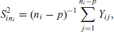
Proof: We prove Theorem 2.1 based on the nonlinear renewal theory[18–21] as follows. By observing (1.3), we can rewrite that
where


where
Let

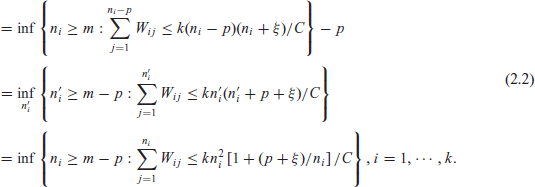
In order to apply the nonlinear renewal theory, we follow the notations in Mukhopadhyay and de Silva[12, pp. 446–449] and rewrite (2.2) as follows: For

where
It follows that for



with

Additionally, we have


By Theorem A.4.2 in Mukhopadhyay and de Silva,[12, p. 448] we claim the following: As

if
Therefore, as

if
We remark that without the fine-tuning parameter ξ in (2.1), the asymptotic bias of the stopping variable N relative to the optimal fixed-sample size C would be given by (by letting ξ = 0 in (2.3)): As

which is approximately k(-1.1828); when k (= number of arms or parallel pieces) is large, the undersampling due to the asymptotic bias would be substantial. We also note that the asymptotic bias (2.4) does not depend on p (= number of explanatory variables in the regression model), although
Suppose k investigators are collecting data from the same population at the same time, but independently of each other. Suppose that
We propose the following stopping time for the fine-tuned parallel piecewise sequential procedure:

where

Termination occurs w.p. 1. Upon termination, we estimate β by

if
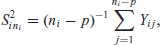
Proof: We prove Theorem 2.2 based on the nonlinear renewal theory[18–21] as follows. Again by observing (1.3), we can rewrite that
where


where
Let

which implies
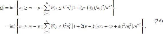
In order to apply the nonlinear renewal theory, we again follow the notations in Mukhopadhyay and de Silva[12, pp. 446-449] and rewrite (2.6) as follows: For

where
It follows that for



with
Additionally, we again have

By Theorem A.4.2 in Mukhopadhyay and de Silva,[12, p. 448] we claim the following: As

if
Therefore, as

if
We remark that without the fine-tuning parameter

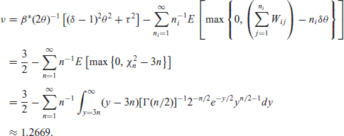
which is approximately k(−0.1166); when k (= number of arms or parallel pieces) is large, the undersampling due to the asymptotic bias could be substantial. We also note that the asymptotic bias (2.8) does not depend on p (= number of explanatory variables in the regression model), although
First, we summarize performances in the case of a FSCR estimation problem and then we analogously report summaries of performances in the case of a MRPE problem. We accomplish both with the help of large-scale simulations that we had undertaken.
FSCR Estimation

Purely Sequential Procedure for FSCR with
and ‘Time’ to Completion Shown in Seconds.
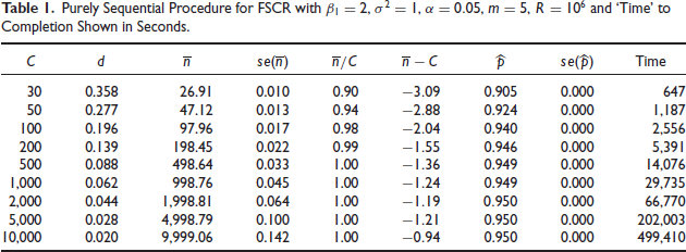
Purely Sequential Procedure for FSCR with
and ‘Time’ to Completion Shown in Seconds.
Fine-tuned Purely Sequential Procedure for FSCR with
and 'Time' to Completion Shown in Seconds.

Parallel Piecewise Sequential Procedure for FSCR with
,
and 'Time' to Completion Shown in Seconds.

Fine-tuned Parallel Piecewise Sequential Procedure for FSCR with
,
and 'Time' to Completion Shown in Seconds.

Parallel Piecewise Sequential Procedure for FSCR with
,
and 'Time' to Completion Shown in Seconds.

Fine-tuned Parallel Piecewise Sequential Procedure for FSCR with
,
and 'Time' to Completion Shown in Seconds.

where the values of 
and the number of replications R = 106. Two scenarios, k = 2,5, are included for the parallel piecewise sequential procedures (with or without fine-tuning).
The term
We note that for a parallel piecewise sequential procedure (with or without fine-tuning) the data collection process is completed as soon as the last operator is done sampling and the final estimation can be given immediately after by pooling data from all arms together. Indeed, the observed runtime of our simulation program is consistent with this intuition. The time-savings are substantial using the parallel piecewise sequential strategy and increase as k increases. For k = 2, we find that the parallel piecewise sequential procedure (with or without fine-tuning) for C = 10,000 takes approximately the same time (around 1.9 × 10⁵ seconds) as the purely sequential procedure for C = 5,000, that the former for C = 2,000 takes approximately the same time (around 2.9 × 10⁴ seconds) as the latter for C = 1,000, and so on. The time savings are even more remarkable when k increases to 5 -the parallel piecewise sequential procedure for C = 10,000 now takes approximately the same time (around 6.4 × 10⁴ seconds) as the purely sequential procedure for C = 2,000, that the former for C = 5,000 takes approximately the same time (around 2.9 × 10⁴ seconds) as the latter for C = 1,000, and so on.
As shown in Tables 1, 3 and 5, respectively, and consistent with (2.4), we find that the estimate
On the other hand, according to Tables 2, 4 and 6, the estimate
Additionally, in all Tables 1–6, we observe that the estimate

Purely Sequential Procedure for MRPE with
and 'Time' to Completion Shown in Seconds.

Purely Sequential Procedure for MRPE with
and 'Time' to Completion Shown in Seconds.
Fine-tuned Purely Sequential Procedure for MRPE with
and 'Time' to Completion Shown in Seconds.

Parallel Piecewise Sequential Procedure for MRPE with
,
and 'Time' to Completion Shown in Seconds.
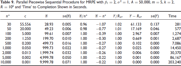
Fine-tuned Parallel Piecewise Sequential Procedure for MRPE with
,
and 'Time' to Completion Shown in Seconds.
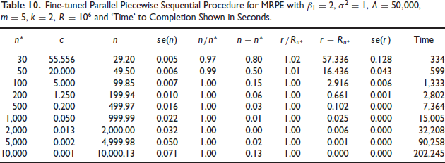
Parallel Piecewise Sequential Procedure for MRPE with
,
and 'Time' to Completion Shown in Seconds.
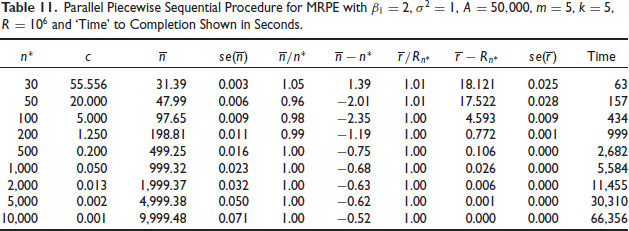
Fine-tuned Parallel Piecewise Sequential Procedure for MRPE with
,
and 'Time' to Completion Shown in Seconds.

Two scenarios,
Again, the term
We again note that for a parallel piecewise sequential procedure (with or without fine-tuning) the data collection process is completed as soon as the last operator is done sampling and the final estimation can be given immediately after by pooling data from all arms together. Indeed, the observed runtime of our simulation program is consistent with this intuition. The time-savings are substantial using the parallel piecewise sequential strategy and increase as k increases. For k = 2, we find that the parallel piecewise sequential procedure (with or without fine-tuning) for
As shown in Tables 7, 9 and 11, respectively, and consistent with (2.8), the estimate
On the other hand, according to Tables 8, 10 and 12, the estimate
Additionally, in all Tables 7–12, we observe that the estimate
The simulations (Section 3) were carried out with only one parameter,
A reviewer rightfully remarked that now-a-days, given the easy and cheap availability of computing resources, it would be great if we included an illustration under simulations with more parameters in the model. We include a brief discussion of the time complexity by highlighting in Table 13 the total run time to completion in the case of Tables 1–12.

In Table 13, we have used the following abbreviations (or legends) for quickly identifying the exact methodology under which each table from Section 3 was constructed:

Understandably, the entries shown in Table 13 correspond to estimation of a single parameter
A personal laptop computer may not be entirely appropriate to run such lengthy jobs since a laptop may seriously overheat after few hours of prolonged number crunching or it may shut itself off or get stuck at some point without warning. Initially, we faced such problems. We ended up using powerful external computing resources to complete the simulations.
In our purely sequential and parallel piecewise sequential estimation strategies, the computation involves repeated evaluation and inversion of matrices at every step of the way as new data arrive. But, matrix inversion is generally an operation with cubic computational complexity so that it has the order
The Wikipedia[22] (
That said, if we included (i)
In the real data illustration included in Section 5, we allow five β parameters, but by mimicking real-life applications, we ran only a single rep instead of one million reps. Moreover, the unknown optimal fixed-sample size
In this section, we illustrate the fine-tuned parallel piecewise sequential procedures (2.1) and (2.5) using a data set from
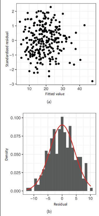
For the purpose of this illustration, we treat the data set of size 252 as our population. The response variable of our interest here is the percentage of body fat 
We note that in this case
(a) Standardized Residual vs. Fitted Value Plot; (b) Histogram of Residuals Superimposed with N(0,19.45) Density Curve.
A fixed-size 95% confidence region for the regression coefficients with 
and
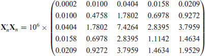
with
Next, let us obtain MRPE for the regression coefficients with 
with
(a) We first saw the advantages of the fine-tuned parallel piecewise sequential sampling techniques for estimation of the unknown mean of a normal population.[1] Now, we have substantiated appreciable benefits of similarly improvised methodologies in the estimation of unknown regression parameters in a linear model. It will be a good idea to explore possible extensions to GLM by substantially moving the area forward way beyond Finster's[10, 11] contributions under fine-tuned parallel piecewise sequential sampling.
(b) There are other possible directions that one may follow in the future to make this methodology more broadly applicable in a number of substantial inference problems. Some potential future research areas may include the development of parallel piecewise sequential strategies (with appropriate fine-tuning) for (i) estimating the location of populations with distributions other than a normal distribution such as a heavy-tailed distribution, (ii) two-sample or even multi-sample estimation problems, and (iii) more general multivariate estimation problems, among others.
(c) We have presented the paper in the context of big data. It may not hit a reader right away what the role of stopping times may be in the context of big data especially since big data are generally synonymous with data sets with no cap on their size. Let us briefly provide our perspective with respect to the relationship between stopping times and big data (and data sets in general), in the context of (sequential) experimental designs for statistical inference. We begin by agreeing that when we talk about big data, we generally mean a data set whose size may be extremely large.
From the experimental designs (for statistical inference) perspective, either in the conventional (nonsequential) setting or in the sequential situation (addressed in our paper here), however, an appropriate sample size will need to be determined first in order for one to collect an appropriate amount of data through the experiment. This will then lead to subsequent statistical inference (e.g., estimation or hypothesis testing) eventually carried out to achieve the predetermined level of precision (for estimation problems) or level of significance (for hypothesis testing problems). Such relevance is aptly validated by the recent contributions of Steland and Chang[25] among other sources.
In the context of sequential experimental designs particularly addressed in our paper, a stopping time (or stopping rule) is a way of determining the most appropriate sample size to achieve the set goal in a statistical inference problem, more specifically, to arrive at a preassigned level of precision (i.e., fixed size) in an FSCR problem or to achieve a minimized risk in a MRPE problem with predetermined 'cost' per data point (unit observation). Generally speaking, if the stopping time (final sample size) is less than the theoretical optimal fixed-sample size, we would be unable to achieve the level of precision required for the FSCR problem or the minimum risk for the MRPE problem. On the other hand, if the stopping time is greater than the optimal fixed-sample size, we would be wasting unnecessary resources (e.g., time and manpower in the traditional sense, data storage and data processing time and cost in the era of big data and cloud computing) by oversampling to achieve the set goal in a statistical inference problem that could have otherwise addressed with less effort, resources, or cost. Therefore, it is critical for one to be able to determine the most appropriate final sample size (stopping time) that is 'just right' by developing a carefully designed stopping rule, on which our paper is focused, in order to most efficiently and effectively perform our hoped statistical inference with the data collected.
(d) A reader may raise issues with our choices of the specific design parameters used in Sections 3 and 4. Those choices made are indeed due to the limitation of computation with the large-scale simulations. It is necessary though to have as many as one million repetitions because only this magnitude (or greater) can produce a reasonably small standard error of the estimate (the difference between final sample size and optimal fixed sample size) when it comes to the last case (row) in each table. However, such limitation under large-scale simulations has nothing to do with the efficiency of our methodology. In practice, instead of incorporating one million or more replications, we would only collect the data points once, and therefore the computation limitation in the sense of the large-scale simulations does not impact application of our methodology in practice.
No simulation study can cover every possible scenario, but a reasonable question may be raised in the sense that we could have added a nonzero intercept and/or an additional predictor. From the perspective of the large-scale simulations, adding either a non-zero intercept or another predictor made the completion of the simulations infeasible given the computation resources we were able to utilize. As a comparison, the time it took to complete the simulations in Mukhopadhyay and Zhang[1] was substantially less. In fact, we were unable to complete the simulations in the present paper with only the computation resources available locally on the laptop (which we did in our paper[1]) and had to resort to the commercial and significantly more powerful Amazon AWS Compute Cloud.
As in all simulations, our simulation study is for illustration purposes only, and it is not intended to be comprehensive in the sense of covering every possible scenario. It is our hope that simulations would not replace the solid and comprehensive theoretical proofs and derivations that we have presented in the earlier sections of the paper.
Footnotes
Acknowledgements
The editor, associate editor and the reviewer shared a number of thoughtful comments. The reviewer also raised a number of penetrating issues which led to a new Section 4 in order for us to address such issues precisely. The totality of their comments helped to improve our presentation. We thank them and we remain grateful to them.
Declaration of Conflicting Interests
The authors declare that there is no conflict of interest.
Funding
The authors received no funding from any source to produce this research.