Fragile Snapshot or Stable Relationships?

Abstract

One of the long-standing criticisms of cross-sectional survey data is that they provide only a contextually driven “snapshot” of attitudes. These attitudes are, the “snapshot critique” contends, highly fragile—subject to significant fluctuation based on events that arise domestically and globally. Although it makes sense that a major event can alter the percentage of people who respond to a given survey question in a particular way, it is less obvious that such an event jeopardizes the validity of multivariate analyses of survey data collected prior to the event. Given the prevalent use of cross-sectional survey data in quantitative political research, this question has significant implications for comparative politics. This study employs survey data from Ukraine before and after the “Orange Revolution” and from Georgia before and after the “Rose Revolution.” Its findings challenge the snapshot critique and support the idea that, even in the wake of a dramatic political event, the underlying relationships among variables measured by survey data can remain quite stable.

Keywords

mass attitudes surveys cross-sectional data snapshot Orange Revolution Rose Revolution

It is frequently said that an opinion poll is a snapshot of public opinion. The problem is that the metaphor is not pushed at all far enough. What needs to be added is that the snapshot may have been under-exposed or over-exposed; the lens may have been telescopic where a wide-angle lens was required or vice versa; the focal length may have been inappropriate; the camera may have been shaken, and so on. In short, the reality of public opinion must not be confused with any set of indicators of it.

—Richard Sinnott (1997, p. 9)

In the summer of 2009, Iranians by the thousands took to the streets to protest what they believed to be a fraudulent presidential election. Encouraged by presidential candidate and main opposition figure Mir Hossein Moussavi, the demonstrations centered in the capital of Tehran but popped up in other large cities across the country. Although the protests were ultimately unsuccessful in ousting President Mahmoud Ahmadinejad from power, the immediate aftermath of the election in Iran had all the markings of the “color revolutions” that had taken place earlier in the decade in countries such as Georgia and Ukraine. Indeed, many called the 2009 events in Iran the “Green Revolution,” from the color used by Moussavi’s campaign.¹

The uprising in Georgia occurred in November 2003, when citizens turned out to protest an election that, temporarily, kept Georgian President Eduard Shevardnadze in office. The protests culminated with a flurry of activity on November 23 and 24. In short order, the “Rose Revolution” led Shevardnadze to resign and a new election to be scheduled. The subsequent election brought Mikheil Saakashvili, Shevardnadze’s opponent in the November election, to power. One year later, the world watched as the Rose Revolution was replayed on a grander scale in Ukraine. The resulting “Orange Revolution” led to a new election and victory for Viktor Yushchenko over the previous “winner,” Viktor Yanukovych. The protests, centered in Kiev but taking place in a number of cities, involved a sizeable portion of the country’s population.

As in the case of the Green Revolution in Iran, the lasting effects of the Rose and Orange Revolutions are open to debate (see Kalandadze & Orenstein, 2009).² Yet they remain defining moments for Georgia and Ukraine. Alongside the other postcommunist “color” revolutions in Serbia and Kyrgyzstan (and additional election protests in Armenia, Azerbaijan, and Belarus), they marked a turning point in the semiauthoritarian politics of much of the postcommunist region. Authoritarian and semiauthoritarian leaders could no longer steal elections without at least some fear of subsequent mass demonstrations leading to the loss of political power.³

The Rose, Orange, and Green Revolutions are also examples of the kind of event that critics of quantitative analysis of cross-sectional survey data point to as a reason one should not trust such data. These data provide, in the oft-used word of these critics, a “snapshot” of a moment in time, which is highly contextual and, therefore, highly fragile. Even day-to-day economic, social, and political events can alter the views of the population on a number of important issues; consequently, an event like the color revolutions could be expected to rock mass attitudes as much as or even more than it does the political system, threatening the validity of data collected prior to the event.

This study is a test of the “snapshot critique” and an alternative view, the “stable relationships argument.” The stable relationships argument accepts the idea that major events like the color revolutions can lead to significant changes in the summary statistics of a dependent variable—such as the average score on a scale of attitudes in Ukraine about ties to Russia—but not in the underlying relationships between that dependent variable and other variables in the model. The snapshot critique, on the other hand, concerns the proposition that major events like the Orange or Rose Revolutions do likely alter the underlying relationships between the dependent variable—again, such as attitudes about Russia in Ukraine—and other variables that one might hypothesize to affect deviations in that variable at the individual level.

This article presents the results of analyses of survey data from 2003 and 2004 in Georgia and 2004 and 2005 in Ukraine to assess the extent to which the color revolutions in these two countries altered key attitudes, and the relationship between these attitudes and factors such as region of residence, ethnicity, and language use. The results point to statistically significant changes in attitudes about Russia and the West. But the analyses also reveal a high degree of stability in the individual-level, multivariate relationships. Although not rejecting the snapshot critique outright, taken as a whole, these findings indicate that researchers should be much more skeptical than they generally are about this common criticism of cross-sectional survey data.

The Conventional Wisdom of Cross-Sectional Survey Data as a “Snapshot”

Cross-sectional studies make up a huge portion of scholarly work utilizing surveys to understand mass attitudes. One of the long-standing criticisms of cross-sectional survey data is that they provide only a contextually driven and highly fragile “snapshot” of attitudes, subject to significant fluctuation based on domestic and global events. It has become widely accepted across subfields of political science that cross-sectional surveys provide only a fleeting glimpse of attitudes.⁴ In an article that otherwise lauds the contributions of survey research to political science, Brady (2000) labels the cross-sectional survey as a “snapshot of a moment in time” (p. 50). Cook and Gronke (2005) concede that their survey from early 2002 “presents a snapshot of opinion at a starkly unusual moment in American politics” (p. 786), whereas Rueda (2005) acknowledges the Eurobarometer data he analyzes provide “only a snapshot of individual preferences” (p. 61).⁵

This belief leads many scholars to dismiss findings from survey data analysis, including tests of individual-level causal hypotheses involving bivariate or multivariate relationships. The snapshot critique is a favorite among comparativists who emphasize the benefits of qualitative methods over quantitative approaches, many of whom are suspicious of all mass survey data analysis. They contend that the fragile nature of survey data makes them ultimately unhelpful in understanding political outcomes. Silverman (1973) summarizes the qualitative critics’ views with the statement that survey data analysis involves “nothing more than a snapshot taken from a misleading angle and frozen in time” (p. 185).

Quantitative scholars with data sets containing variables measured over time, particularly those engaged in panel data research, often join in the qualitative critics’ attacks. In a work on tolerance in Russia, Gibson (2002) argues that his panel data allow a more accurate causal story than cross-sectional analyses. Hilton and Patrick (1970) are more forceful, stating, “Few methodological generalizations are as widely accepted as the superiority of longitudinal data over cross-sectional data” (p. 15).

Mainstream political science research methods textbooks and other guides for those interested in survey research have also come to portray the snapshot critique as empirical fact, helping perpetuate the idea by passing it on to the next generation of political scientists. In their discussion of cross-sectional survey research, for example, Manheim, Rich, and Willnat (2002) assert, “Cross-sectional surveys offer a snapshot of a moving target. They are best suited to exploratory and descriptive studies” (p. 122). Even the American Statistical Association (2009), on its webpage on survey research careers, states, “Social research depends heavily on surveys, which can provide a snapshot . . . of social trends.”

The “Stable Relationships Argument” Versus the “Snapshot Critique”

Considerations of whether findings from cross-sectional survey data analysis can be expected to hold up over time generate two distinct arguments about why one might be concerned, in the face of a major political event, about using cross-sectional survey data to estimate a hypothesized set of multivariate relationships (represented by Equation 1.1).

Y = B_{0} + B_{1} X_{1} + B_{2} X_{2} + B_{3} X_{3} + \dots + B_{N} X_{N} + U

(1.1)

Where,

B₀ = the Y intercept

B₁ = the coefficient term for X₁, representing the change in Y from a unit change in X₁, with the effects of the other variables held constant

B₂ = the coefficient term for X₂, representing the change in Y from a unit change in X₂, with the effects of the other variables held constant

B₃ = the coefficient term for X₃, representing the change in Y from a unit change in X₃, with the effects of the other variables held constant

B_N = the coefficient term for X_N, representing the change in Y from a unit change in X_N (the final variable of the hypothesized multivariate relationship), with the effects of the other variables held constant

U = the stochastic error term

The Stable Relationships Argument

The first argument accepts that survey data-based estimations of the dependent variable’s value—that is, the percentage of respondents who answer a certain question in a certain way—may be unstable over time. The idea that a major event can alter, perhaps quite noticeably, a population’s political attitudes associated with that event makes sense. It would have been strange, for example, if the portion of Americans who felt that the government should take steps to be more vigilant against terrorism had not risen notably after the 9/11 attacks. Like the broader snapshot critique, it assumes the respondents’ answers to the question(s) used to measure the dependent variable before and after the event (e.g., 9/11) can shift collectively, leading to a change in the average value of the dependent variable (e.g., a higher score on a scale of support for aggressive measures to protest against terrorism).

The key to this first argument about the stability of survey data is that, as opposed to the snapshot critique, it does not assume that the relationships between the dependent variable and the independent variables also change. Consequently, this view of cross-sectional survey data is labeled the stable relationships argument. Starting with the hypothesized set of multivariate relationships in Equation 1.1, the stable relationships argument contends that a major event would likely cause the intercept term in the model to change but not the coefficients on the independent variables. It is represented formally by Equation 1.2.

Y = (B_{0} + C_{0}) + B_{1} X_{1} + B_{2} X_{2} + B_{3} X_{3} + \dots + B_{N} X_{N} + U

(1.2)

Where C₀ = the change in the intercept term because of the occurrence of the important event.

The Snapshot Critique

The second view, and the main thrust of the concept of cross-sectional data as a “snapshot,” is that individual-level relationships among variables are unstable over time. This view is labeled the snapshot critique. It contends that findings from survey data analysis involving ordinary least squares (OLS) regression or other multivariate statistical techniques are as fragile as the quantitative measures (e.g., the mean) of the dependent variable. Again using the set of multivariate relationships in Equation 1.1, the snapshot critique holds not only that a major event would lead the intercept in Equation 1.1 to shift but also that that event would generate important changes in the slopes of the hypothesized linear relationships. The formal statement of the snapshot critique is presented in Equation 1.3.

Y = (B_{0} + C_{0}) + (B_{1} + C_{1}) X_{1} + (B_{2} + C_{2}) X_{2} + (B_{3} + C_{3}) X_{3} + \dots + (B_{N} + C_{N}) X_{N} + U

(1.3)

Where,

C₀ = the change in the intercept term because of the occurrence of the important event

C₁ = the change in the coefficient term on X₁ because of the occurrence of the important event

C₂ = the change in the coefficient term on X₂ because of the occurrence of the important event

C₃ = the change in the coefficient term on X₃ because of the occurrence of the important event

C_N = the change in the coefficient term on X_N (the final variable of the hypothesized multivariate relationship) because of the occurrence of the important event

Note that this formalization of the snapshot critique does not distinguish between a change in a coefficient that magnifies an already notable effect and a change in a coefficient that signals an effect disappearing or a change in a coefficient’s sign, which indicates that a positive relationship has become a negative one or vice versa. Yet these distinctions are important conceptually. If a major event deepens an already-strong causal relationship, this is a nontrivial result, but it is conceptually distinct from, and arguably less important than, a situation in which the event leads a strong causal relationship to disappear or change from a positive one to a negative one.

The Failure to Test Adequately the Snapshot Critique and Stable Relationships Arguments

The snapshot critique and the stable relationships argument represent two very different ideas about how a major event could alter underlying causal relationships. Unfortunately, as the quotations highlighted earlier in the article indicate, promoters of the idea of cross-sectional survey data fragility generally fail to distinguish between the two views, and partly as a result, scholars generally fail to test their respective validity. Even when researchers have had the opportunity to analyze multiple sets of cross-sectional data over time, they have almost never employed appropriate tests to ascertain the stability of the cross-sectional, multivariate findings.

The closest that comparative politics scholars have come to testing the snapshot critique is Whitefield’s (2003) analysis of Russian attitudes toward the environment.⁶ In this study, he examines data from 1993, 1995, 1996, 1998, and 2001, establishing the change in attitudes about addressing pollution and making limited comparisons of multivariate models for 1993 and 2001. Whitefield also estimates a model of support for environmentalism using the pooled data by including dummy terms for the years of the surveys. He claims this is done to understand the “degree to which the difference over time in support for environmental policies is accounted for by changes in the effects of class, education, household circumstances, and other social factors” (Whitefield, 2003, p. 101, italics added). However, Whitehead fails to include interaction terms between year of the surveys and the other variables in the model, instead comparing only a full model of the dummy variables for the survey year and a number of demographic factors to a model of the survey year dummy variables alone. This choice, in combination with the dependent variable itself not representing change in environmental attitudes, makes it impossible to assess whether the effects of the socioeconomic variables change over time. Without the interaction terms, his model is underspecified for what he seeks to do.

The Rose Revolution and the Orange Revolution as Real-World Experiments

This study investigates the effects of two dramatic upheavals as a test of stable relationships argument and the snapshot critique. The tests involve analyses of survey data on views toward Russia and the West before and after the Rose and Orange Revolutions. Although there are limitations to the methodological approach of this study that further studies should address, these color revolutions provide a “tough test” of the stable relationships hypothesis and an “easy test” for the snapshot critique. As a result, findings contrary to the snapshot critique would be surprising.

Methodological Overview

This study’s data from Georgia were collected in August 2003 and February 2004, by the Georgian Opinion Research Business International (GORBI). GORBI is a leading survey organization in Georgia and the only Georgian member organization of Gallup International. The survey was conducted throughout Georgia (except for the regions of Abkhazia and Ossetia). GORBI utilized a multistage, random probability sampling method during respondent selection, yielding a sample of 1,000 respondents in August 2003 and 1,500 respondents in February 2004.

Data were also collected in Ukraine in August–September 2004 and April 2005 by the Kiev International Institute of Sociology (KIIS). KIIS is one of the best known and most respected Ukrainian survey organizations. The data were obtained as part of KIIS’s national omnibus survey project, which involves surveys every few months across Ukraine. The sample was selected through a multistage stratified probability technique representative of the adult (18 years and older) population of Ukraine. All oblasti plus Krym (Crimea) and the city of Kyiv (Kiev) were represented in the samples.⁷

Using the pre- and postrevolution data, individual-level relationships between the dependent variables and a number of demographic variables on which researchers of postcommunist mass attitudes generally focus are estimated. (See the appendix for the coding of the independent variables). The analysis of these data takes place in two parts, corresponding to the stable relationships argument and the snapshot critique. One could eyeball the results of separate OLS regression model estimates for the pre- and postrevolution data, looking for important changes in the intercept term (as a test of the stable relationships argument) and the coefficients on the independent variables (the snapshot critique). The more statistically elegant way to determine whether the color revolution in each country affected individual-level multivariate relationships, however, is to analyze a pooled set of the pre- and postrevolution data.

In this approach, one compares a “base model,” with a number of explanatory variables and a dummy variable term representing the postrevolution survey data, to a second model that includes interactions between the postrevolution data variable and the variables in the original model. The statistical significance of the coefficient on the base model’s dummy variable term representing the postrevolution survey data provides a test of the extent to which attitudes collectively shifted as a result of the color revolution. The coefficients on the interaction terms indicate the extent to which the underlying relationships between the dependent variable and the independent variables in the base model changed as a result of the color revolution. An F test of the improved fit of the interaction terms model assesses the extent to which the color revolution led to a significant overall change in the underlying relationships, even if few individual coefficients were statistically significant.

Tough Tests: The Rose and Orange Revolutions and Views of Russia and the West

Given its drama and obvious impact on the Georgian political landscape, the Rose Revolution provides the kind of tough test that researchers hope for when analyzing a research question in a single country. In this case, though, it is a tough test of the stable relationships argument and an easy test for the snapshot critique. If we would expect underlying causal patterns to be shaken by an event, it would be an event like the Rose Revolution. The Rose Revolution was also an international moment. While the protests were building in Georgia, the United States issued a public statement condemning the election as fraudulent. European Union representatives made similar statements, and EU officials traveled to Georgia in the months between Shevardnadze’s resignation and Saakashvili’s inauguration. Russian officials, meanwhile, played a key role in brokering Shevardnadze’s resignation. Thus, all three international powers, the United States, the EU, and Russia, were players in the Rose Revolution, and all three countries’ actions would have been viewed favorably by the bulk of the Georgian public. Because this activity most likely altered attitudes toward all three in the minds of Georgians, it makes sense to examine attitudes toward these important foreign powers.⁸

The Orange Revolution’s protests, related presidential elections, and campaigns leading up to these elections were in many ways even more dramatic than their counterparts in Georgia. The protests and their aftermath were momentous (for more analysis of the Orange Revolution, see Aslund & McFaul, 2006), and the Orange Revolution became a defining moment for Ukraine. Like the Rose Revolution in Georgia, it provides a tough test of the idea that mass attitudes and their causal patterns can remain stable in the face of important happenings—and, by the same token, an easy test for the snapshot critique.

Examining attitudes in Ukraine toward relations with Russia continues the “tough test”–“easy test” theme. Ukraine’s relations with Russia were a central issue in the presidential campaigns before and after the Orange Revolution protests. The Russian government openly supported Yanukovych, with such encouragement extending to financial support and tactical advice. There was also widespread speculation that elements of the Russian government were involved in the disfiguring dioxin poisoning of Yushchenko during the campaign. Whether or not the Russian government was directly involved, many Ukrainians believed that it was. Consequently, though the Ukrainian public was deeply divided over relations with Russia prior to the Orange Revolution, a modest shift in attitudes (with the Ukrainian population being less supportive of close ties to Russia) would be expected.

In both the Georgian and Ukrainian analyses, the dependent variable related to Russia comes from a single question asked in both the pre- and postrevolution surveys. In the Georgian surveys, the question asked about the respondent’s overall opinion toward Russia: “Please use this card to tell me your overall opinion about Russia. Do you have a very good, fairly good, fairly bad, or very bad opinion of Russia?” Answers were coded to produce a –10 to 10 scale, with 10 representing a very good opinion of Russia, 5 being fairly good, 0 representing “don’t know,” –5 being a fairly bad opinion of Russia, and –10 representing a very bad opinion of Russia. Similar questions were asked about the United States and the EU, and these questions were coded and combined into a single 20 to –20 scale on attitudes toward the West.

In Ukraine, the question on Russia focuses on relations between Ukraine and the Russian Federation: “What kind of relationship would you like to see between Ukraine and Russia? (1) They must be the same as with other states—as with the West; (2) Ukraine and Russia must be independent, but friendly states; (3) Ukraine and Russia must unite into one state.” The answers were coded to produce a –10 to 10 scale, with 10 representing a desire for Ukraine and Russia to unite into a single country, 0 being independent but friendly, and –10 representing relations with Russia as with any other country. “Don’t know” responses (totaling only 3%) were excluded.

In any study, decisions are made for methodological and practical reasons. The decision to look at only one survey question on views of Russia from both Georgia and Ukraine falls into the latter category. The questionnaires were designed by others for purposes different from those of this study. The purpose of the both the GORBI surveys and the KIIS omnibus surveys is to assess questions deemed particularly pressing at the moment. Thus, the questions rarely overlapped on the pre- and postrevolution surveys. In both the Georgian and Ukrainian cases, the surveys provided only one identical question about the respondents’ views toward Russia.

Results and Discussion

Georgia

In the case of Georgia, there were four OLS estimations: a base model and interactions model with attitudes about Russia as the dependent variable and a base model and interactions model with views of the United States and the EU as the dependent variable. The independent variables in the models are a set of socioeconomic and demographic variables common to studies of postcommunist mass attitudes.⁹ Table 1 contains the results of the OLS regression estimation of Model 1 and Model 2 on views toward Russia; coefficients significant at p ≤ .05 are in bold. The size and statistical significance of the coefficients in Model 1 point to the importance of region, ethnic identity, type of residence, education level, and age group on attitudes about Russia.¹⁰

Table 1.

Ordinary Least Squares Regression Results Pooled Data From Georgia, With and Without 2004 Interactions

Dependent variable: Opinion of Russia:^a Min = -10, Max = 10, M = 2.82
	Model 1 (base)				Model 2 (2004 interactions)
Independent variables	B	SE	T-stat	Sig.	B	SE	T-stat	Sig.
Constant term	1.064	0.370	2.874	.004	1.773	0.518	3.421	.001
Region (West Region)
Tbilisi	−0.059	0.328	−0.181	.857	0.516	0.513	1.003	.316
South Region	2.225	0.303	7.350	.000	2.180	0.482	4.521	.000
East Region	1.745	0.310	5.632	.000	2.430	0.489	4.975	.000
Ethnic Identity (Ethnic Georgian)
Ethnic Russian or Ukrainian	1.665	0.694	2.399	.017	2.621	1.246	2.104	.035
Ethnic Armenian	3.033	0.658	4.610	.000	4.116	1.005	4.094	.000
Ethnic Azeri	0.437	0.854	0.511	.609	−1.602	1.363	−1.175	.240
Other Ethnic Group	2.944	1.341	2.195	.028	2.954	1.395	2.117	.034
Language (Georgian Speaker)
Russian Speaker	0.998	0.740	1.350	.177	1.417	1.149	1.234	.217
Type of Residence (Village)
City	−0.714	0.256	−2.792	.005	−2.545	0.406	−6.265	.000
Education Level (Low Level of Educ.)
Medium Educ. Level	0.135	0.319	0.422	.673	0.696	0.422	1.647	.100
High Educ. Level	−0.667	0.334	−1.996	.046	−0.372	0.416	−0.893	.372
Age Group (60 and older)
50-59	−0.432	0.349	−1.236	.217	−0.853	0.564	−1.512	.131
40-49	−0.746	0.316	−2.358	.018	−1.218	0.496	−2.456	.014
30-39	−0.166	0.331	−0.501	.616	−0.413	0.513	−0.804	.421
18-29	−1.178	0.323	−3.651	.000	−1.799	0.523	−3.437	.001
Male	0.415	0.215	1.932	.052	0.768	0.337	2.276	.023
2004 Survey	2.503	0.239	10.471	.000	1.935	0.800	2.418	.016
Interaction Terms
Region
Tbilisi × 2004					−0.942	0.665	−1.418	.156
South × 2004					−0.024	0.617	−0.039	.969
East × 2004					−1.246	0.631	−1.976	.048
Ethnic Identity
Russian or Ukrainian × 2004					−1.483	1.497	−0.991	.322
Armenian × 2004					−1.805	1.324	−1.363	.173
Azeri × 2004					3.363	1.747	1.925	.054
Other Ethnic × 2004					5.739	5.425	1.058	.290
Language
Russian × 2004					−0.421	1.510	−0.279	.780
Type of Residence
City × 2004					2.974	0.521	5.707	.000
Education Level
Medium Educ. × 2004					−1.332	0.703	−1.895	.058
Higher Educ. × 2004					−1.204	0.736	−1.636	.102
Age Group
50-59 × 2004					0.705	0.717	0.984	.325
40-49 × 2004					0.836	0.644	1.299	.194
30-39 × 2004					0.387	0.672	0.576	.565
18-29 × 2004					0.971	0.666	1.458	.145
Male × 2004					−0.454	0.436	−1.040	.298
	N = 2,500, Adj. R² = .120, SEE = 5.274				N = 2,500, Adj. R² = .135, SEE = 5.228

SEE = standard error of the estimate. Coefficients significant at p ≤ .05 are in bold.

“Please use this card to tell me your overall opinion about Russia. Do you have a very good, fairly good, fairly bad, or very bad opinion of Russia?” Very good opinion of Russia = 10, fairly good = 5, don’t know = 0, fairly bad = -5, very bad = -10.

The positive coefficient sign on the dummy variable representing 2004 respondents is consistent with the more positive mean value on the dependent variable scale in 2004 compared to 2003.¹¹ The statistically significant coefficient on this variable in Model 1 is consistent with the stable relationships argument. It does not, however, tell us whether the Rose Revolution altered the pattern of relationships between the dependent variable and the other variables in Model 1. For that, one must examine the difference between Model 1 and Model 2. The latter model includes a large number of interaction terms, which come from multiplying each of the variables in Model 1 by the dummy variable representing the 2004 survey. If the events surrounding the Rose Revolution had an impact on the extent to which the demographic variables in Model 1 affected views of Russia, one would expect a number of the interaction terms in Model 2 to be statistically significant. Instead, only two of the interaction term coefficients are significant at the p ≤ .05 level.

It is possible that the small number of statistically significant interaction term coefficients is hiding an improved overall model fit. The final part of the analysis of attitudes in Georgia about Russia, therefore, includes an examination of the statistical significance of the overall improvement of the model resulting from the addition of the interaction terms. This is done through an F test on the improved fit generated by the additional variables, presented in Table 2. The statistics in Table 2 are consistent with the snapshot critique. The F statistic captures the overall statistical significance of the model, and the “change in F” captures the improved fit resulting from the additional variables in Model 2 that are excluded from Model 1. Thus, the statistical significance of the “change in F” statistic points to a collective change in the causal patterns related to opinions about Russia following the Rose Revolution.

Table 2.

R² Change From the Addition of the 2004 Interaction Variables

	Model summary				Change statistics
Model	R	R ²	Adj. R²	SEE	ΔR²	ΔF	df1	df2	Sig. ΔF
1	.354	.126	.120	5.274	.126	20.939	17	2477	.000
2	.383	.146	.135	5.228	.021	3.753	16	2461	.000

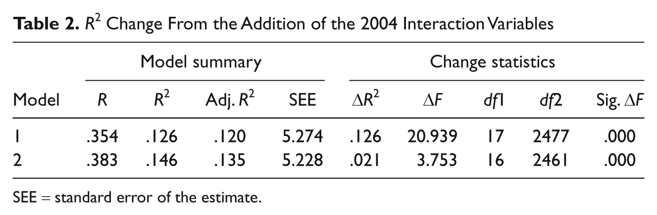
SEE = standard error of the estimate.

Table 3 contains the results of the estimation of the models of opinion about the United States and the EU. Models 3 and 4 contain the same independent variables as those of Models 1 and 2, respectively. With the exception of the regional variables, the coefficients on the variables in Model 3 tell a similar story to those of Model 1. Ethnic identity, type of residence, education level, and age group all have significant dummy term coefficients.¹² The significant coefficient on the 2004 survey variable again provides support for the stable relationships argument.

Table 3.

Ordinary Least Squares Regression Results Pooled Data From Georgia, With and Without 2004 Interactions

Dependent variable: Opinion of United States and European Union:^a Min = −20, Max = 20, M = 8.79
	Model 3 (base)				Model 4 (2004 interactions)
Independent variables	B	SE	T-stat	Sig.	B	SE	T-stat	Sig.
Constant Term	4.339	0.521	8.334	.000	4.074	0.735	5.544	.000
Region (West Region)
Tbilisi	−0.714	0.461	−1.549	.121	−0.939	0.729	1.288	.198
South Region	0.537	0.426	1.261	.207	0.799	0.684	1.169	.243
East Region	0.679	0.436	1.555	.120	1.427	0.696	2.052	.040
Ethnic Identity (Ethnic Georgian)
Ethnic Russian or Ukrainian	−1.849	0.977	1.893	.058	−1.819	1.773	−1.026	.305
Ethnic Armenian	−2.187	0.925	−2.364	.018	−2.932	1.426	−2.056	.040
Ethnic Azeri	−5.624	1.216	−4.624	.000	−5.840	1.997	−2.924	.003
Other Ethnic Group	−2.581	1.886	−1.369	.171	−2.840	1.979	−1.435	0.151
Language (Georgian Speaker)
Russian Speaker	−0.234	1.048	−0.224	.823	1.473	1.665	0.885	.376
Type of Residence (Village)
City	0.880	0.360	2.444	.015	1.127	0.578	1.951	.051
Education Level (Low Level of Educ.)
Medium Educ. Level	1.014	0.449	2.258	.024	0.902	0.600	1.504	0.133
High Educ. Level	1.230	0.470	2.616	.009	0.880	0.591	1.488	.137
Age Group (60 and older)
50–59	1.618	0.492	3.292	.001	1.683	0.802	2.100	.036
40–49	1.165	0.445	2.620	.009	0.897	0.703	1.276	.202
30–39	1.927	0.465	4.141	.000	1.919	0.729	2.631	.009
18–29	1.904	0.454	4.196	.000	3.012	0.742	4.056	.000
Male	0.412	0.303	1.362	.173	0.110	0.479	0.230	.818
2004 Survey	3.233	0.337	9.606	.000	3.257	1.134	2.871	.004
Interaction Terms
Region
Tbilisi × 2004					0.374	0.942	0.397	.692
South × 2004					−0.421	0.874	−0.482	.630
East × 2004					−1.194	0.896	−1.332	.183
Ethnic Identity
Russian or Ukrainian × 2004					0.122	2.128	0.057	.954
Armenian × 2004					1.404	1.878	0.748	.455
Azeri × 2004					0.315	2.527	0.125	.901
Other Ethnic × 2004					2.298	7.690	0.299	.765
Language
Russian × 2004					−3.403	2.168	−1.621	.105
Type of Residence
City × 2004					−0.348	0.740	−0.470	.638
Education Level
Medium Educ. × 2004					0.660	0.996	0.663	.508
Higher Educ. × 2004					1.083	1.044	1.037	.300
Age Group
50–59 × 2004					−0.159	1.017	−0.156	.876
40–49 × 2004					0.367	0.913	0.403	.687
30–39 × 2004					−0.161	0.954	−0.169	.866
18–29 × 2004					−1.977	0.945	−2.093	.036
Male × 2004					0.480	0.619	0.775	.438
	N = 2,500, Adj. R² = .096, SEE = 7.41				N = 2,500, Adj. R² = .097, SEE = 7.41

SEE = standard error of the estimate. Coefficients significant at p ≤ .05 are in bold.

“Please use this card to tell me your overall opinion about the United States. Do you have a very good, fairly good, fairly bad, or very bad opinion of the United States?” Very good opinion of U.S. = 10, fairly good = 5, don’t know = 0, fairly bad = −5, very bad = −10. “Please use this card to tell me your overall opinion about the European Union. Do you have a very good, fairly good, fairly bad, or very bad opinion of the European Union?” Very good opinion of EU = 10, fairly good = 5, don’t know = 0, fairly bad = −5, very bad = −10. Dependent variable scale was created from summing these two variables.

Table 4 contains the results of the comparison in model fit between Model 3 and 4. The comparison of these two models tells a very different story from the comparison of Model 1 and Model 2. Despite the inclusion of 16 additional variables, the unadjusted R² statistic improved by only .007. More telling is the adjusted R² statistic, which takes into account the number of variables in the model, increasing by only .001.

Table 4.

R² Change From the Addition of the 2004 Interaction Variables

	Model summary				Change statistics
Model	R	R ²	Adj. R²	SEE	ΔR²	ΔF	df1	df2	Sig. ΔF
3	.319	.102	.096	7.41	.102	16.510	17	2473	.000
4	.330	.109	.097	7.41	.007	1.255	16	2457	.218

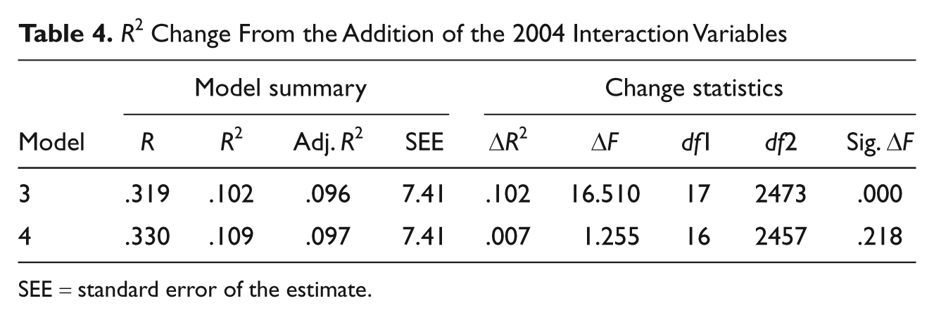
SEE = standard error of the estimate.

This finding is consistent with the most important finding presented in Table 4: the lack of statistical significance at p ≤ .05 for the “change in F” statistic for Model 4. This result means that one cannot reject the null hypothesis of no improvement in the explanatory power of Model 4 over Model 3. Thus, the addition of the interaction terms, which collectively represent the effect of the events that occurred between November 2003 and February 2004, appears unwarranted, a blow to the snapshot critique.

Ukraine

Taking the same approach to the analysis of the data from Ukraine results in two models: a base model (Model 5) and an interactions model (Model 6) of attitudes regarding Ukraine’s proper relations with Russia. Again, the estimation technique is OLS regression. However, with the dependent variable having only three ordinal categories, ordinal logit and probit estimations of the two models would be appropriate. The OLS results are presented instead for two reasons. First, in terms of both the variables that had statistically significant coefficients and the lack of statistical significance from the addition of the set of interaction terms, the results of the ordinal probit and logit estimations are essentially identical to those of the OLS estimations.¹³ Second, logit and probit coefficients are more difficult to interpret, and readers may be more familiar with F tests on sets of OLS coefficients than on the analogous likelihood ratio comparisons in the logit and probit analyses. Table 5 contains the OLS results.

Table 5.

Ordinary Least Squares Regression Results Pooled Data From Ukraine, With and Without 2005 Interactions

Dependent variable: View of Proper Relations with Russia:^a Min = −10, Max = 10, M = 0.995
	Model 5 (base)				Model 6 (2005 interactions)
Independent variables	B	SE	T-stat	Sig.	B	SE	T-stat	Sig.
Constant Term	−0.617	0.348	−1.773	.076	−0.575	0.466	−1.234	.217
Region (West Region)
West-central Region	2.970	0.274	10.829	.000	2.492	0.407	6.128	.000
East-central Region	3.558	0.325	10.944	.000	3.162	0.491	6.442	.000
South Region	4.228	0.365	11.589	.000	3.284	0.554	5.932	.000
East Region	4.373	0.364	12.027	.000	3.098	0.539	5.749	.000
Ethnic Identity (Ethnic Ukrainian)
Other Ethnic Group	−0.098	0.435	−0.455	.649	−0.345	0.599	−0.576	.565
Ethnic Russian	1.666	0.244	6.839	.000	1.650	0.362	4.563	.000
Language (Ukrainian Speaker)
Ukrainian and Russian Speaker	0.908	0.293	3.105	.002	1.255	0.440	2.856	.004
Russian Speaker	1.124	0.297	3.777	.000	1.409	0.438	3.219	.001
Type of Residence (Village)
Small Town	0.118	0.331	0.356	.722	0.687	0.551	1.248	.212
Small Sized City	−0.474	0.414	−1.146	.252	−0.232	0.572	−0.406	.685
Medium Sized City	−0.154	0.291	−0.531	.595	−0.049	0.420	−0.116	.907
Large City	0.438	0.237	1.847	.065	0.248	0.338	0.733	.464
Very Large City	−0.893	0.280	−3.192	.001	−0.683	0.395	−1.731	.084
Education Level (Low Level of Educ.)
Medium Educ. Level	−0.980	0.282	−3.487	.001	−0.578	0.397	−1.454	.146
High Educ. Level	−1.730	0.324	−5.344	.000	−1.414	0.460	−3.073	.002
Age Group (60 and older)
50-59	−0.087	0.293	−0.298	.766	−0.104	0.422	−0.246	.806
40-49	−0.800	0.272	−2.943	.003	−0.762	0.389	−1.956	.051
30-39	−0.560	0.281	−1.994	.046	−0.602	0.408	−1.478	.140
18-29	−1.047	0.267	−3.920	.000	−1.134	0.388	−2.919	.004
Personal Economic Situation (Very Poor)
Poor	−0.229	0.232	−0.985	.325	−0.374	0.319	−1.171	.242
Okay	−0.811	0.266	−3.051	.002	−0.888	0.374	−2.376	.018
Good to Very Good	−1.059	0.371	−2.851	.004	−0.745	0.492	−1.512	.131
Male	−0.296	0.168	−1.758	.079	−0.038	0.241	−0.158	.874
2005 Survey	−0.493	0.168	−2.939	.003	−0.541	0.689	−0.786	.432
Interaction Terms
Region
West-central × 2005					0.795	0.554	1.434	.152
East-central × 2005					0.582	0.659	0.882	.378
South × 2005					1.639	0.741	2.212	.027
East × 2005					2.351	0.737	3.190	.001
Ethnic Identity
Other Ethnic × 2005					0.297	0.878	0.339	.735
Ethnic Russian × 2005					−0.134	0.492	−0.272	.785
Language
Ukr. & Russian × 2005					−0.463	0.592	−0.784	.433
Russian × 2005					−0.403	0.603	−0.669	.504
Type of Residence
Small Town × 2005					−0.835	0.694	−1.204	.229
Small Sized City × 2005					−0.772	0.842	−0.916	.360
Medium Sized City × 2005					−0.249	0.589	−0.423	.672
Large City × 2005					0.478	0.476	1.004	.315
Very Large City × 2005					−0.424	0.561	−0.757	.449
Education Level
Medium Educ. × 2005					−0.833	0.565	−1.475	.140
Higher Educ. × 2005					−0.701	0.649	−1.080	.280
Age Group
50-59 × 2005					0.057	0.586	0.097	.922
40-49 × 2005					−0.013	0.546	−0.025	.980
30-39 × 2005					0.128	0.565	0.226	.821
18-29 × 2005					0.131	0.537	0.243	.808
Personal Economic Situation
Poor × 2005					0.314	0.470	0.667	.505
Okay × 2005					0.260	0.539	0.482	.630
Good to V. Good × 2005					−0.750	0.760	−0.986	.324
Male × 2005					−0.504	0.337	−1.495	.135
	N = 3,800, Adj. R² = .182, SEE = 5.09				N = 3,800, Adj. R² = .184, SEE = 5.08

SEE = standard error of the estimate. Coefficients significant at p ≤ .05 are in bold.

“What kind of relationship would you like to see between Ukraine and Russia?” They must be the same as with other states, as in the West = -10; Ukraine and Russia must be independent, but friendly states = 0; Ukraine and Russia must unite into one state = 10.

The coefficient patterns in Model 5 capture what scholars of Ukrainian mass attitudes have typically found: the importance of region and, to a lesser extent, ethnicity and language. Given that the dependent variable scale ranged from only –10 to 10, the sizes of some of these statistically significant coefficients also indicate important effects on the dependent variable. In addition, there were statistically significant coefficients on the education level variables, with the negative sign on the coefficients indicating that better educated residents of Ukraine were less supportive of close ties to Russia than the excluded, comparison category: those with low levels of education. A number of the age group dummy variables were also statistically significant, with the negative coefficient signs in this case indicating less attachment to Russia among the young than among the old (the excluded, comparison category was those older than age 60) as well as two of the economic well-being variables (with the coefficients indicating that the better off are less supportive of close ties with Russia than the very poor). Similar to the estimations of the models using the data from Georgia, the coefficient on the dummy term for the postrevolution (2005) data is significant, though in this case negative.¹⁴ This result again provides support for the stable relationships argument, as it is evidence of an across-the-board shift in attitudes about Ukraine’s relationship with Russia.

Whether the Orange Revolution generated shifts in the slopes of the various linear relationships is indicated by the interaction terms and the significance of the improved model fit resulting from the inclusion of the interaction terms. Only two of the interaction terms are significant at p ≤ .05 (those involving the east and south region dummy variables).¹⁵ These large and positive coefficients do indicate that the Orange Revolution deepened the already strong divide—readily apparent in analyses of survey data before the Orange Revolution—between the west of Ukraine and its east and south. They do not, however, tell a new story about region and attitudes about Russia in Ukraine.

Table 6 presents the results of the comparison of Models 5 and 6. As Table 6 shows, despite the addition of 23 variables, the unadjusted R² statistic increased by only .006.¹⁶ The adjusted R² also increased, but by only.002. This gives some indication, albeit very weak, that the fit of Model 6 is superior to that of Model 5. However, the key result in Table 6 is the lack of statistical significance at the p ≤ .05 level for the “change in F” statistic for Model 6. In the analysis of views about Ukraine’s relations with Russia, taking into account the events of late 2004 and early 2005 in Ukraine provides no statistically significant improvement. This is, once again, a blow to the snapshot critique.

Table 6.

R² Change From the Addition of the 2005 Interaction Variables

	Model summary				Change statistics
Model	R	R ²	Adj. R²	SEE	ΔR²	ΔF	df1	df2	Sig. ΔF
5	.433	.187	.182	5.08619	.187	36.235	24	3775	.000
6	.440	.194	.184	5.08149	.006	1.304	23	3752	.151

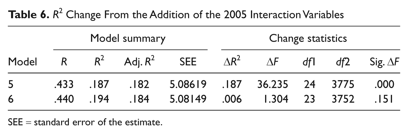
SEE = standard error of the estimate.

Comparing the Tests of the Stable Relationships Argument and the Snapshot Critique

The statistical significance of the postrevolution survey dummy term in Models 1, 3, and 5 points to a general shift in attitudes following the Rose and Orange Revolutions. These shifts support the stable relationship argument’s assumption that major events can alter patterns in the percentage of respondents choosing a particular answer to a given question. On the other hand, the models of multivariate relationships that included interaction terms provide limited support at best for the snapshot critique. Only one of the three models with the interaction terms explains significantly more of the variance of the dependent variable than the models without the interaction terms. Moreover, the individual coefficients on the interaction terms generally lack statistical significance.¹⁷

In Georgia, the east region became less supportive of Russia following the Rose Revolution, but the east remained more pro-Russian than Georgia’s west. The only interaction term coefficient that indicates a major change from 2003 is the one on the city × 2004 variable, which points to city residents becoming much more pro-Russian after the events of the Rose Revolution. In the case of attitudes toward the United States and the EU, only one interaction term—the 18–29 age group × 2004 variable—is statistically significant, and the model itself does not provide a significantly improved fit compared to the base model.

In Ukraine, the coefficients on the east region × 2005 and the south region × 2005 interaction terms indicate that the Orange Revolution deepened the divide between residents of the west and those of the east and south. Yet this divide was already well established by earlier analyses of Ukrainian mass attitudes. The story that survey data prior to the Orange Revolution tell about what drives variation in support for close ties to Russia looks very much like the story that survey data after the Orange Revolution convey as well.

Conclusion

This study’s results should give pause to those who reject statistical analysis of cross-sectional survey data as a contextually fragile, even futile endeavor. Individual-level relationship patterns were more stable than conventional wisdom would predict. Such findings suggest a need for further study, and subsequent studies should address this one’s methodological limitations. A multiquestion measure of the dependent variables, for example, should be used. The reduced form model used in the present study also relies on variables—region, language, ethnicity, and so on—that themselves are unlikely to change in response to a significant event. Although demographic factors are often the variables of interest to researchers, analyzing a more complex model with demographic and attitudinal explanatory variables could be informative. Having data closer to the start and end of the event in question would also benefit future studies. The length of time between the collection of the data sets analyzed in this study (3 months on each side of the Rose Revolution and 4 months on each side of the Orange Revolution) may have been too long to capture the revolutions’ immediate effects, allowing old causal patterns to reemerge.¹⁸ Additional data collected at different points in time on each side of a major event may point to greater variation in how stable underlying relationships are than the data did in this study.

In addition, even if the findings in this article had categorically rejected the snapshot critique, this would not imply that understanding multivariate, individual-level relationships requires us to look only once at cross-sectional data. Replication and verification are at the heart of all branches of science, and although one should be careful about assuming how fragile the findings from survey data are, most causal relationships involving political attitudes and behavior can be expected to change eventually.

Moreover, not all criticisms of cross-sectional survey data concern the idea that such data are fragile and unstable. Certain research questions simply cannot be easily answered through cross-sectional data.¹⁹ If one’s research question specifically concerns changes in a dependent variable over time, cross-sectional data from sources like mass surveys are, indeed, quite limited in what they can offer. Just as Bowen and Wiersema (1999) warn against assuming that underlying parameters are unchanging over time, however, one should not throw the baby out with the bath water by assuming that, regardless of the topic of study and the level of analysis, major changes are inevitable in the short or medium term. Although beyond the scope of this study, the most interesting questions for further research on the snapshot critique involve which kinds of events are more likely than others to change existing causal relationships and what perceptual or behavioral micro foundations those events are triggering that other events are not.

This study’s results indicate that scholars should not reject findings from cross-sectional survey data analyses simply because the data are cross-sectional. In the cases of the Rose and Orange Revolutions, analyses of the pre- and postevent survey data indicate that the underlying individual-level relationships across these data are not akin to separate snapshots of a busy city street—a constantly shifting setting that looks quite different even minutes later. Instead, the multivariate patterns in the cross-sectional data analyzed in this study come across as something more like a painting of a rural landscape, which offers a relatively faithful, long-term representation of a scene that might change, but slowly and only somewhat, over time.

Footnotes

Appendix

Acknowledgements

The author thanks Merab Pachulia and Vladimir Paniotto for providing access to the data analyzed in this article. Jeff Drope, John Jackson, John McAdams, and Brian Silver offered helpful comments on the statistical analysis in the article, and Katherine Arnold, Brooke Chichakly, Yuliya Humphrey, Anne Mozena, Lauren Reeves, Craig Shockley, Lilia Yakova, and Ivana Zivanovic provided valuable research assistance.

The author(s) declared no potential conflicts of interest with respect to the authorship and/or publication of this article.

The author(s) received no financial support for the research and/or authorship of this article.

Notes

References

Ambrosio

Thomas

. (2007). Insulating Russia from a colour revolution: How the Kremlin resists regional democratic trends. Democratization, 14, 232-252.

American Statistical Association. (2009). Surveys. Retrieved from http://www.amstat.org/careers/surveys.cfm

Aslund

Anders

McFaul

Michael

. (Eds.). (2006). Revolution in orange: The origins of Ukraine’s democratic breakthrough. Washington, DC: Carnegie Endowment for International Peace.

Barrington

Lowell

Faranda

Regina

. (2009). Reexamining region, ethnicity, and language in Ukraine. Post-Soviet Affairs, 25, 232-256.

Bowen

Harry P.

Wiersema

Margarethe F.

(1999). Matching method to paradigm in strategy research: Limitations of cross-sectional analysis and some methodological alternatives. Strategic Management Journal, 20, 625-636.

Brady

Henry E.

(2000). Contributions of survey research to political science. PS: Political Science and Politics, 33, 47-57.

Cook

Timothy E.

Gronke

Paul

. (2005). The skeptical American: Revisiting the meanings of trust in government and confidence in institutions. Journal of Politics, 67, 784-803.

Franklin

Charles H.

Kosaki

Liane C.

(1989). Republican schoolmaster: The U.S. Supreme Court, public opinion, and abortion. American Political Science Review, 83, 751-771.

Gibson

James L.

(2002). Becoming tolerant? Short-term changes in Russian political culture. British Journal of Political Science, 32, 309-334.

10.

Gordon

Philip H.

Chollet

Derek

. (2005, August 18). Don’t let the Rose Revolution wilt. YaleGlobal. Retrieved from http://yaleglobal.yale.edu/content/dont-let-rose-revolution-wilt

11.

Hilton

Thomas L.

Patrick

Cathleen

. (1970). Cross-sectional versus longitudinal data: An empirical comparison of mean differences in academic growth. Journal of Educational Measurement, 7, 15-24.

12.

Inglehart

Ronald

. (1998). The renaissance of political culture. American Political Science Review, 82, 1203-1230.

13.

Kalandadze

Katya

Orenstein

Mitchell A.

(2009). Electoral protests and democratization beyond the color revolutions. Comparative Political Studies, 42, 1403-1425.

14.

Manheim

Jarol B.

Rich

Richard C.

Willnat

Lars

. (2002). Empirical political analysis: Research methods in political science. New York, NY: Longman.

15.

Perez

Orlando J.

(1999). Public opinion and the future of U.S.–Panama relations. Journal of Interamerican Studies and World Affairs, 41(3), 1-34.

16.

Pierson

Paul

. (2005). The study of policy development. Journal of Policy History, 17, 34-51.

17.

Rueda

David

. (2005). Insider-outsider politics in industrialized democracies: The challenge to social democratic parties. American Political Science Review, 99, 61-74.

18.

Sinnott

Richard

. (1997). European public opinion and security policy (Chaillot Papers No. 28). Paris, France: Institute for Security Studies of the WEU.

19.

Silverman

David

. (1973). Methodology and meaning. In Paul

Filmer

Michael

Phillipson

David

Silverman

David

Walsh

(Eds.), New directions in sociological theory (pp. 183-202). Cambridge, MA: MIT Press.

20.

Whitefield

Stephen

. (2003). Russian mass attitudes towards the environment, 1993–2001. Post-Soviet Affairs, 19, 95-113.