Marginal Effects in Interaction Models: Determining and Controlling the False Positive Rate

Abstract

When a researcher suspects that the marginal effect of $x$ on $y$ varies with $z$ , a common approach is to plot $\partial y / \partial x$ at different values of $z$ along with a pointwise confidence interval generated using the procedure described in Brambor, Clark, and Golder to assess the magnitude and statistical significance of the relationship. Our article makes three contributions. First, we demonstrate that the Brambor, Clark, and Golder approach produces statistically significant findings when $\partial y / \partial x = 0$ at a rate that can be many times larger or smaller than the nominal false positive rate of the test. Second, we introduce the interactionTest software package for R to implement procedures that allow easy control of the false positive rate. Finally, we illustrate our findings by replicating an empirical analysis of the relationship between ethnic heterogeneity and the number of political parties from Comparative Political Studies.

Keywords

political parties quantitative methods interaction

Introduction

Much of the recent empirical work in political science¹ has recognized that causal relationships between two variables $x$ and $y$ are often changed—strengthened or weakened—by contextual variable $z$ . Such a relationship is commonly termed interactive. The substantive interest in these relationships has been coupled with an ongoing methodological conversation about the appropriate way to test hypotheses in the presence of interaction. The latest additions to this literature, particularly King, Tomz, and Wittenberg (2000); Ai and Norton (2003); Braumoeller (2004); Brambor, Clark, and Golder (2006); Kam and Franzese (2007); Berry, DeMeritt, and Esarey (2010); and Berry, Golder, and Milton (BGM: 2012), emphasize visually depicting the marginal effect of $x$ on $y$ at different values of $z$ (with a confidence interval [CI] around that marginal effect) to assess whether that marginal effect is statistically and substantively significant. The statistical significance of a multiplicative interaction term is seen as neither necessary nor sufficient for determining whether $x$ has an important or statistically distinguishable relationship with $y$ at a particular value of $z$ . That is, although a statistically significant product term is sufficient for concluding that $\partial y / \partial x$ is different at different values of $z$ (Kam & Franzese, 2007, p. 50), it cannot tell us whether $\partial y / \partial x$ is statistically distinguishable from zero at any particular value of $z$ .

A paragraph from Brambor et al. (2006) summarizes the current state of the art:

The analyst cannot even infer whether $x$ has a meaningful conditional effect on $y$ from the magnitude and significance of the coefficient on the interaction term either. As we showed earlier, it is perfectly possible for the marginal effect of $x$ on $y$ to be significant for substantively relevant values of the modifying variable $z$ even if the coefficient on the interaction term is insignificant. Note what this means. It means that one cannot determine whether a model should include an interaction term simply by looking at the significance of the coefficient on the interaction term. Numerous articles ignore this point and drop interaction terms if this coefficient is insignificant. In doing so, they potentially miss important conditional relationships between their variables. (p. 74)

In short, they recommend including a product term $x z$ in linear models where interaction between $x$ and $z$ is suspected, then examining a plot of $\partial y / \partial x$ and its 95% CI over the range of $z$ in the sample.² If the CI does not include zero for any value of $z$ , one should conclude that $x$ and $y$ are statistically related (at that value of $z$ ), with the substantive significance of the relationship given by the direction and magnitude of the $\partial y / \partial x$ estimate. It is hard to exaggerate the impact that the methodological advice given in Brambor et al. (2006) has had on the discipline: The article has been cited over 3,300 times as of August 2016. Similar advice is given in Braumoeller (2004, pp. 815-818, especially Figure 2), which has been cited over 660 times in the same time frame.

Our article makes three contributions to the study of interactive relationships. First, we highlight a hazard with the Brambor, Clark, and Golder procedure: The reported $α$ level of CIs and hypothesis tests constructed using the procedure can be inaccurate because of a multiple comparison problem (Abdi, 2007; Sidak, 1967). The source of the problem is that adding an interaction term $z$ to a model like $y = β_{0} + β_{1} x$ is analogous to dividing a sample data set into subsamples defined by the value of $z$ , each of which (under the null hypothesis that $\partial y / \partial x = 0$ ) has a separate probability of a false positive (i.e., falsely rejecting the null hypothesis when the null is true). For example, if $z$ is dichotomous ( $z \in {0, 1}$ ), estimating a model like $y = β_{0} + β_{1} x + β_{2} z + β_{3} x z$ is analogous to estimating $y = β_{0} + β_{1} x$ twice, once for data where $z = 0$ and once for data where $z = 1$ , with two opportunities for $β_{1}$ to be found statistically significant by chance. A similar problem is already well recognized in the ANOVA for nominal treatment factors (e.g., Kutner, Nachtsheim, Neter, & Li, 2004, Section 19.9). In contrast, the methods that are described in Brambor et al. (2006) construct a pointwise CI (typically using a two-tailed $α = . 05$ ); “pointwise” indicates that the CIs are constructed for each individual value of $z$ without considering the joint coverage of the CI for all values of $z$ . That is, the CI for each value of $z$ assumes a single draw from the sampling distribution of the marginal effect of interest. As a result, these CIs can either be too wide or too narrow to conduct the tests that scholars wish to perform³: Plotting $\partial y / \partial x$ over values of $z$ and reporting any statistically significant relationship tend to result in overconfident tests, while plotting $\partial y / \partial x$ over $z$ and requiring statistically significant relationships at multiple values of $z$ tend to result in underconfident tests.⁴ The latter scenario may occur when, for example, a theory predicts that $\partial y / \partial x > 0$ for $z = 0$ and $\partial y / \partial x < 0$ for $z = 1$ , and we try to jointly confirm these predictions in a data set.

Second, we offer researchers guidance on strategies that are effective and ineffective at controlling the false positive rate when examining interaction relationships. Our primary recommendation is for researchers to simply be aware that marginal effects plots generated using a given $α$ could be over- or underconfident, and thus to take a closer look if results are at the margin of statistical significance. When overconfidence is an issue, researchers can control the false discovery rate (FDR) in marginal effects plots by adapting the procedure of Benjamini and Hochberg (1995)⁵; we provide code to accomplish this in R (R Core Team, 2017) in our new interactionTest package. Researchers can also control the familywise error rate (FWER) of these plots using a simple $F$ test (Kam & Franzese, 2007, pp. 43-51), although this procedure is more conservative and less powerful than controlling the FDR. We rule out one possible solution for overconfidence: Researchers cannot solve the problem by conditioning inference on the statistical significance of the interaction term (assessing $\partial y / \partial x$ for multiple $z$ only when the product term indicates interaction in the data generating process [DGP]) because this procedure results in an excess of false positives.⁶ In situations where marginal effects plots with pointwise CIs (like those in Brambor et al., 2006) would be underconfident, such as when researchers are jointly testing multiple theoretical predictions, a bootstrapping procedure allows researchers to construct marginal effects plots with CIs that have appropriate coverage. We provide R code for this procedure in the interactionTest package.

Finally, we demonstrate the application of our recommendations by reexamining Clark and Golder (2006), one of the first published applications of the hypothesis testing procedures described in Brambor et al. (2006). The authors’ original analysis, published in Comparative Political Studies, indicates that ethnic heterogeneity increases the number of political parties only when electoral district magnitude (in number of seats) is sufficiently large. Our reanalysis indicates that the authors’ claims cannot be supported by a procedure that sets the FWER at 90% and are only partially supported by a procedure that sets the FDR at 90%. The strongest support for the authors’ hypothesis comes from a procedure that jointly tests the authors’ multiple predictions to achieve maximum power while controlling the joint false positive rate, illustrating (a) the usefulness of research designs that combine theory and empirics and (b) the sensitivity of Clark and Golder’s results to prespecification of theoretical expectations.

Interaction Terms and the Multiple Comparison Problem

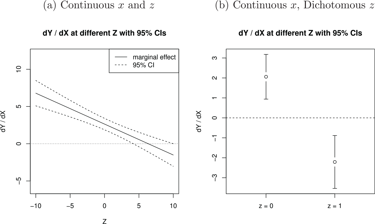
We begin by considering the following question: When we aim to assess the marginal effect of $x$ on $y$ $(\partial y / \partial x)$ at different values of a conditioning variable $z$ , how likely will at least one marginal effect come up statistically significant by chance alone? In the context of linear regression, Brambor et al. (2006) recommend (a) estimating a model with $x$ , $z$ , and $x z$ terms, then (b) plotting the estimated $\partial y / \partial x$ from this model for different values of $z$ along with 95% CIs. If the CIs exclude zero at any $z$ , they conclude that the evidence rejects the null hypothesis that $\partial y / \partial x = 0$ for this value of $z$ (Brambor et al., 2006, pp. 75-76). Figure 1 depicts sample plots for continuous and dichotomous $z$ variables; the 95% CI excludes zero in both examples (for values of $z ≲ 4$ in the continuous case, and for both $z = 0$ and $1$ in the dichotomous case), and so both samples can be interpreted as evidence for a statistical relationship between $x$ and $y$ .

Figure 1.

Sample marginal effects plots in the style of Brambor, Clark, and Golder (2006).

Our goal is to assess the false positive rate of this test procedure—that is, the proportion of the time that this procedure detects a statistically significant $\partial y / \partial x$ for at least one value of $z$ when the null hypothesis that $(\partial y / \partial x | z) = 0$ is true for all $z$ . If the false positive rate is greater than the nominal size of the test, $α$ , then the procedure is overconfident: The CI covers $(\partial y / \partial x | z) = 0$ for all $z$ less than $(1 - α)$ proportion of the time when the null is true. If the false positive rate is less than $α$ , then the procedure is underconfident: The CI could be narrower while still covering $(\partial y / \partial x | z) = 0$ for all $z$ with probability $(1 - α)$ when this null is true. In the case of the Brambor et al. (2006) procedure, the question is whether the 95% CIs in Figure 1 exclude zero for at least one value of $z$ more or less than 5% of the time under the null hypothesis that $(\partial y / \partial x | z) = 0$ for all values of $z$ .

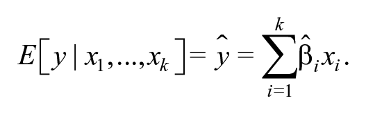
As most applied researchers know, when a $t$ test is conducted—for example, for a coefficient or marginal effect in a linear regression model—the $α$ level of that $t$ test is only valid for a single $t$ test conducted on a single coefficient or marginal effect.⁷ It is not valid for simultaneously testing the statistical significance of multiple coefficients. Consider the example of a simple linear model:

E [y | x_{1},\dots, x_{k}] = \hat{y} = \sum_{i = 1}^{k} {\hat{β}}_{i} x_{i} .

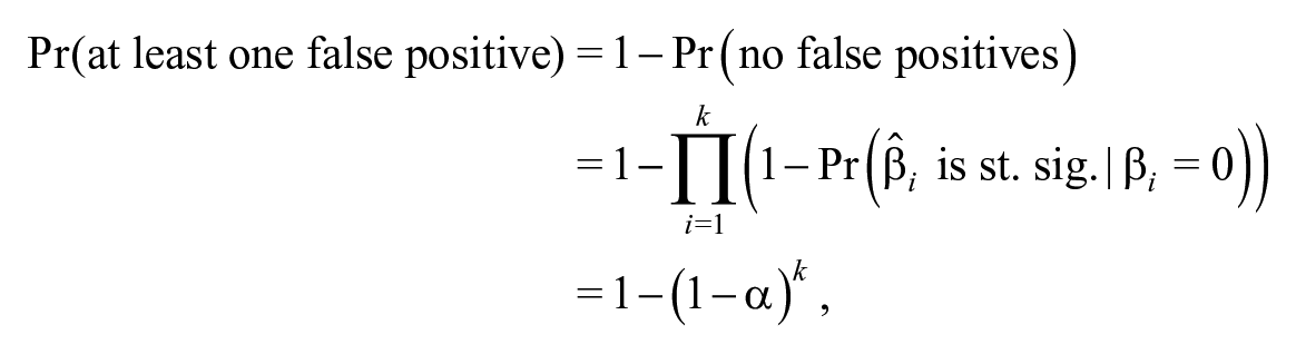
If a researcher conducts two $t$ tests on two different $β$ coefficients, there is usually a greater than 5% chance that either or both of them comes up statistically significant by chance alone when $α = . 05$ . In fact, if a researcher enters $k$ variables that have no relationship to the dependent variable into a regression, the probability that at least one of them comes up significant (in statistically independent tests) is

\begin{matrix} \Pr (at least one false positive) = 1 - \Pr (no false positives) \\ = 1 - \prod_{i = 1}^{k} (1 - \Pr ({\hat{β}}_{i} is st . sig . | β_{i} = 0)) \\ = 1 - {(1 - α)}^{k}, \end{matrix}

so if the researcher tries five $t$ tests on five irrelevant variables, the probability that at least one of them will be statistically significant is ≈ $22.6 %$ , not $5 %$ . This is an instance of the multiple comparison problem; the problem is associated with a long literature in applied statistics (Hochberg, 1988; Holm, 1979; Lehmann, 1957a, 1957b; Rom, 1990; Shaffer, 1995).

The same logic applies to testing one irrelevant variable in $k$ different samples. Indeed, the canonical justification for frequentist hypothesis testing involves determining the sampling distribution of the test statistic, then calculating the probability that a particular value of the statistic will be generated by a sample of data produced when the null hypothesis of the test is true. Thus, if a researcher takes a particular sample data set and randomly divides it into $k$ subsamples, the probability of finding a statistically significant effect in at least one of these subsamples by chance is also $1 - {(1 - α)}^{k}$ when the null of no relationship is true and the hypothesis tests are statistically independent.

Interaction Terms Create a Multiple Comparison Problem: The Case of a Dichotomous Interaction Variable

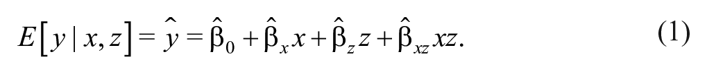
Interacting two variables in a linear regression model effectively divides a sample into subsamples, thus creating the multiple comparison problem described above. This is a well-recognized problem in the context of ANOVA, where textbooks recommend multiple comparison adjustment when examining the marginal effect of one treatment condition whose effect is moderated by another treatment (e.g., Kutner et al., 2004, Section 19.9). The simplest and most straightforward example is a linear model with a continuous independent variable $x$ interacted with a dichotomous independent variable $z \in {0, 1}$ :

E [y | x, z] = \hat{y} = {\hat{β}}_{0} + {\hat{β}}_{x} x + {\hat{β}}_{z} z + {\hat{β}}_{x z} x z .

(1)

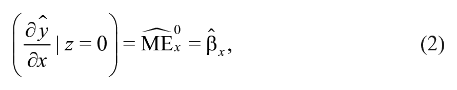
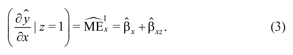
A researcher wants to know whether $x$ has a statistically detectable relationship with $y$ , as measured by the marginal effect of $x$ on $E [y | x, z]$ from Equation 1: $\partial \hat{y} / \partial x$ . Let ${\hat{ME}}_{x}$ be shorthand notation for $\partial \hat{y} / \partial x$ and ${\hat{ME}}_{x}^{z_{0}}$ be shorthand notation for $(\partial \hat{y} / \partial x | z = z_{0})$ , where $z_{0}$ is any possible value of $z$ . Because $x$ is interacted with $z$ , this means that the researcher needs to calculate CIs for two quantities:

(\frac{\partial \hat{y}}{\partial x} | z = 0) = {\hat{ME}}_{x}^{0} = {\hat{β}}_{x},

(2)

(\frac{\partial \hat{y}}{\partial x} | z = 1) = {\hat{ME}}_{x}^{1} = {\hat{β}}_{x} + {\hat{β}}_{x z} .

(3)

These (pointwise) CIs can be created by doing any of the following: (a) by analytically calculating $var ({\hat{ME}}_{x}^{0})$ and $var ({\hat{ME}}_{x}^{1})$ using the variance–covariance matrix of the $\hat{β}$ estimates, (b) by simulating draws of $\hat{β}$ out of the asymptotically normal distribution of $\hat{β}$ and constructing simulated CIs of Equations 2 and 3, or (c) by bootstrapping estimates of $\hat{β}$ via repeated resampling of the data set and constructing CIs using the resulting $\hat{β}$ estimates.

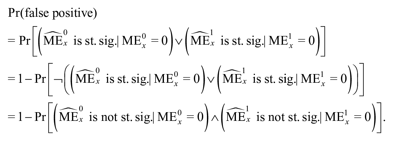
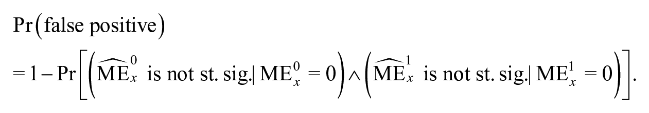
Common practice, and the practice recommended by Brambor et al. (2006), is to report the estimated statistical and substantive significance of the relationship between $x$ and $y$ at all values of the interaction variable $z$ . Unfortunately, the practice inflates the probability of finding at least one statistically significant ${\hat{ME}}_{x}^{z_{0}}$ . A model with a dichotomous interaction term creates two significance tests in each of the two subsamples, one for which $z = 0$ and one for which $z = 1$ . This means that the probability that at least one statistically significant ${\hat{ME}}_{x}^{z_{0}}$ will be found and reported under the null hypothesis that $M E_{x}^{0} = M E_{x}^{1} = 0$ is

\begin{array}{l} \Pr (false positive) \\ = \Pr [({\hat{ME}}_{x}^{0} is st . sig . | {ME}_{x}^{0} = 0) \lor ({\hat{ME}}_{x}^{1} is st . sig . | {ME}_{x}^{1} = 0)] \\ = 1 - \Pr [\neg (({\hat{ME}}_{x}^{0} is st . sig . | {ME}_{x}^{0} = 0) \lor ({\hat{ME}}_{x}^{1} is st . sig . | {ME}_{x}^{1} = 0))] \\ = 1 - \Pr [({\hat{ME}}_{x}^{0} is not st . sig . | {ME}_{x}^{0} = 0) \land ({\hat{ME}}_{x}^{1} is not st . sig . | {ME}_{x}^{1} = 0)] . \end{array}

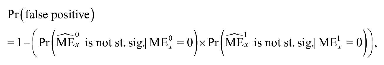
If the two marginal effects (and their associated statistical significance tests) in the second term are unrelated, as when the sample is split into two based on the value of $z$ and a regression separately estimated on each subsample, then we can rewrite this as

\begin{array}{l} \Pr (false positive) \\ = 1 - (\Pr ({\hat{ME}}_{x}^{0} is not st . sig . | {ME}_{x}^{0} = 0) \times \Pr ({\hat{ME}}_{x}^{1} is not st . sig . | {ME}_{x}^{1} = 0)), \end{array}

where ${ME}_{x}^{z_{0}}$ is the true value of $\partial y / \partial x$ when $z = z_{0}$ . If the test for each individual marginal effect has size $α$ , this finally reduces to

\Pr (false positive) = 1 - {(1 - α)}^{2} .

(4)

The problem is immediately evident: The probability of accidentally finding at least one statistically significant ${\hat{ME}}_{x}^{z_{0}}$ is no longer equal to $α$ . For a conventional two-tailed $α = . 05$ , this means there is a $1 - {(1 - . 05)}^{2} =$ 9.75% chance of concluding that at least one of the marginal effects is statistically significant even when ${ME}_{x}^{0} = {ME}_{x}^{1} = 0$ . Stated another way, the test is less conservative than indicated by $α$ . The problem is even worse for a larger number of discrete interactions; if $z$ has three categories, for example, there is a $1 - {(1 - . 05)}^{3} \approx 14.26 %$ chance of a false positive in this scenario.

To confirm this result, we conduct a simulation analysis to assess the false positive rate for a linear regression model. For each of 10,000 simulations, 1,000 observations of a continuous dependent variable $y$ are drawn from a linear model:

y = 0.2 + u,

where $u \sim Φ (0, 1)$ . Covariates $x$ and $z$ are independently drawn from the uniform distribution between 0 and 1, with $z$ dichotomized by rounding to the nearest integer. By construction, neither covariate has any relationship to $y$ , that is, the null hypothesis that ${ME}_{x}^{z_{0}} = {ME}_{z}^{x_{0}} = 0$ is correct for all values of $z_{0}$ and $x_{0}$ . We then estimate a linear regression of the form:

\hat{y} = {\hat{β}}_{0} + {\hat{β}}_{1} x + {\hat{β}}_{2} z + {\hat{β}}_{p} x z,

and calculate the predicted marginal effect ${\hat{ME}}_{x}^{z_{0}}$ for the model when $z = 0$ and $1$ .

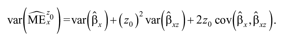
The statistical significance of the marginal effects ${\hat{ME}}_{x}^{z_{0}}$ is assessed in three different ways. First, we use the appropriate analytic formula to calculate the variance of ${\hat{ME}}_{x}^{z_{0}}$ using the variance–covariance matrix of the estimated regression; this is

var ({\hat{ME}}_{x}^{z_{0}}) = var ({\hat{β}}_{x}) + {(z_{0})}^{2} var ({\hat{β}}_{x z}) + 2 z_{0} cov ({\hat{β}}_{x}, {\hat{β}}_{x z}) .

This enables us to calculate a pointwise 95% CI using the critical $t$ statistic for a two-tailed $α = . 05$ test in the usual way. Second, we simulate 1,000 draws out of the asymptotic (multivariate normal) distribution of $\hat{β}$ for the regression, calculate ${\hat{ME}}_{x}^{z_{0}}$ at $z_{0} = 0$ and $1$ for each draw, and select the 2.5th and 97.5th percentiles of those calculations to form a 95% CI at each value of $z_{0}$ . Finally, we construct 1,000 bootstrap samples (with replacement) for each data set, estimate $\hat{β}$ in each bootstrap sample, calculate ${\hat{ME}}_{x}^{z_{0}}$ at $z_{0} = 0$ and $1$ using the $\hat{β}$ from each bootstrap sample, and use the 2.5th and 97.5th percentiles of the calculated marginal effects to construct a 95% CI at each value of $z_{0}$ .

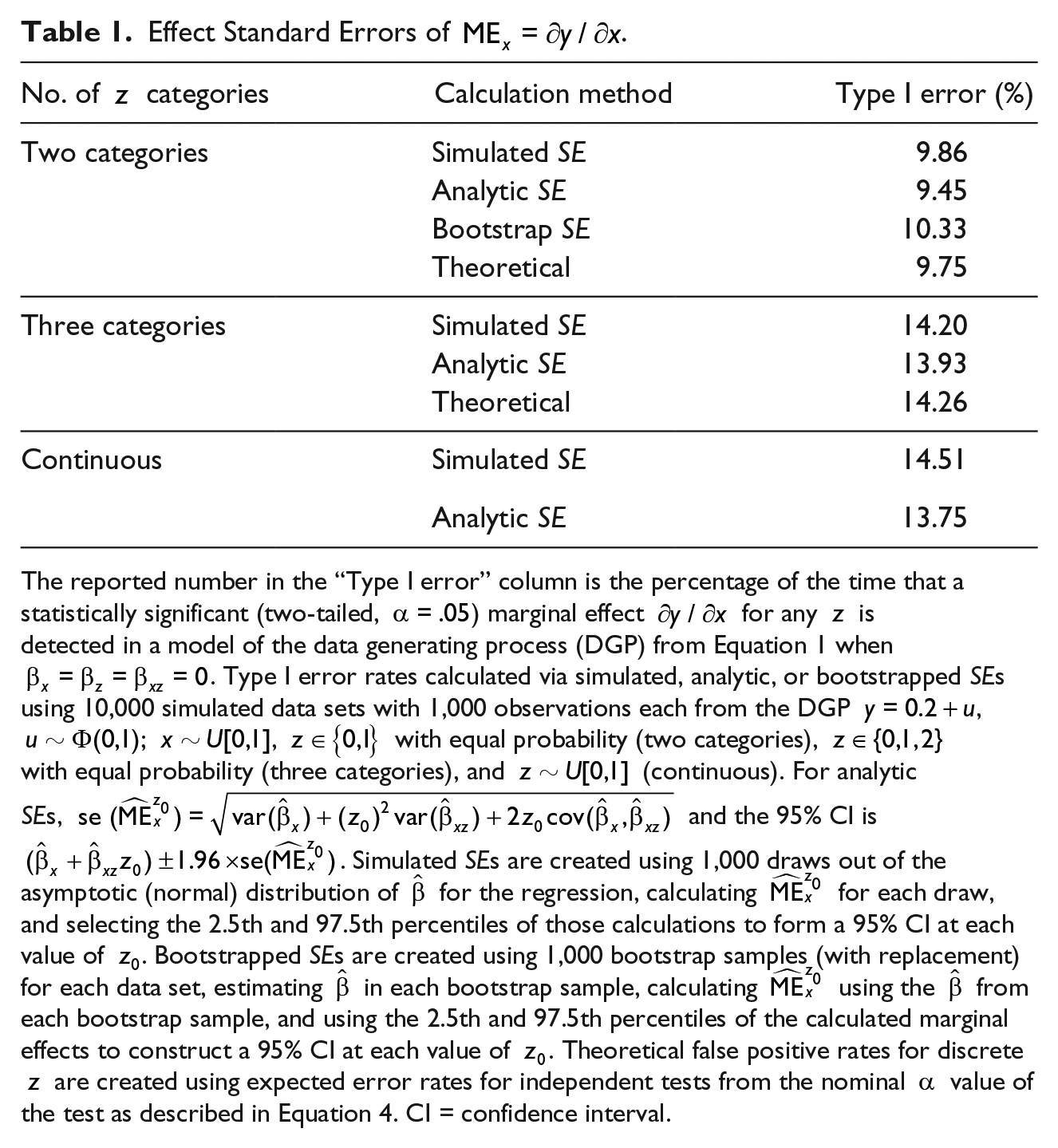
The results for a model with a dichotomous $z$ variable are shown in Table 1. The table shows that, no matter how we calculate the standard error of the marginal effect, the probability of a false positive (Type I error) is considerably higher than the nominal $α = . 05$ and close to the theoretical expectation for statistically independent tests.

Table 1.

Effect Standard Errors of ${ME}_{x} = \partial y / \partial x$ .

No. of $z$ categories	Calculation method	Type I error (%)
Two categories	Simulated SE	9.86
	Analytic SE	9.45
	Bootstrap SE	10.33
	Theoretical	9.75

Three categories	Simulated SE	14.20
	Analytic SE	13.93
	Theoretical	14.26

Continuous	Simulated SE	14.51
	Analytic SE	13.75

The reported number in the “Type I error” column is the percentage of the time that a statistically significant (two-tailed, $α = . 05$ ) marginal effect $\partial y / \partial x$ for any $z$ is detected in a model of the data generating process (DGP) from Equation 1 when $β_{x} = β_{z} = β_{x z} = 0$ . Type I error rates calculated via simulated, analytic, or bootstrapped SEs using 10,000 simulated data sets with 1,000 observations each from the DGP $y = 0.2 + u$ , $u \sim Φ (0, 1)$ ; $x \sim U [0, 1]$ , $z \in {0, 1}$ with equal probability (two categories), $z \in {0, 1, 2}$ with equal probability (three categories), and $z \sim U [0, 1]$ (continuous). For analytic SEs, $se ({\hat{ME}}_{x}^{z_{0}}) = \sqrt{var ({\hat{β}}_{x}) + {(z_{0})}^{2} var ({\hat{β}}_{x z}) + 2 z_{0} cov ({\hat{β}}_{x}, {\hat{β}}_{x z})}$ and the 95% CI is $({\hat{β}}_{x} + {\hat{β}}_{x z} z_{0}) \pm 1.96 \times se ({\hat{ME}}_{x}^{z_{0}})$ . Simulated SEs are created using 1,000 draws out of the asymptotic (normal) distribution of $\hat{β}$ for the regression, calculating ${\hat{ME}}_{x}^{z_{0}}$ for each draw, and selecting the 2.5th and 97.5th percentiles of those calculations to form a 95% CI at each value of $z_{0}$ . Bootstrapped SEs are created using 1,000 bootstrap samples (with replacement) for each data set, estimating $\hat{β}$ in each bootstrap sample, calculating ${\hat{ME}}_{x}^{z_{0}}$ using the $\hat{β}$ from each bootstrap sample, and using the 2.5th and 97.5th percentiles of the calculated marginal effects to construct a 95% CI at each value of $z_{0}$ . Theoretical false positive rates for discrete $z$ are created using expected error rates for independent tests from the nominal $α$ value of the test as described in Equation 4. CI = confidence interval.

Continuous Interaction Variables

The multiple comparison problem and resulting overconfidence in hypothesis tests for marginal effects can be worsened when a linear model interacts a continuous independent variable $x$ with a $z$ variable that has more than two categories. For example, an interaction term between $x$ and a continuous variable $z$ implicitly cuts a given sample into many small subsamples for each value of $z$ in the range of the sample. By subdividing the sample further, we create a larger number of chances for a false positive.

To illustrate the potential problem with overconfidence in models with more categories of $z$ , we repeat our Monte Carlo simulation with statistically independent $x$ and $z$ variables using a three-category $z \in {0,1,2}$ (where each value is equally probable) and a continuous $z \in [0, 1]$ (drawn from the uniform distribution) instead of a dichotomous $z$ . Bootstrapping is computationally intensive and yields no different results than the other two processes when $z$ is dichotomous; we therefore only assess simulated and analytic standard errors for the three-category and continuous $z$ cases. The results are shown in Table 1.

As before, the observed probability of a Type I error is far from the nominal $α$ probability of the test. A continuous $z$ tends to have a higher false positive rate than a dichotomous $z$ (≈ $14 %$ compared with ≈ $10 %$ under equivalent conditions), and roughly equivalent to a three-category $z$ .

Statistical Interdependence Between Marginal Effects Estimates

In the section above, we assumed that marginal effects estimates (and related statistical significance tests) at different values of $z$ are uncorrelated. But if the significance tests of ${\hat{ME}}_{x}^{0}$ and ${\hat{ME}}_{x}^{1}$ are related when $z$ is dichotomous, we would expect correlation between the statistical significance of marginal effects estimates when, for example, $x$ and $z$ are themselves correlated, or when $β_{x}$ and $β_{x z}$ are stochastic and correlated. In this case, the probability of a false positive result is

\begin{array}{l} \Pr (false positive) \\ = 1 - \Pr [({\hat{ME}}_{x}^{0} is not st . sig . | {ME}_{x}^{0} = 0) \land ({\hat{ME}}_{x}^{1} is not st . sig . | {ME}_{x}^{1} = 0)] . \end{array}

If $({\hat{ME}}_{x}^{0} is not st . sig . | {ME}_{x}^{0} = 0)$ and $({\hat{ME}}_{x}^{1} is not st . sig . | {ME}_{x}^{1} = 0)$ are perfectly correlated, then we expect the joint probability that both occur to be equal to either individual probability that one occurs ( $1 - α$ ) and therefore $\Pr (false positive) = 1 - (1 - α) = α$ . In that case, the individual tests have correct size. As their correlation falls, the joint probability that both occur falls below $(1 - α)$ as the proportion of the time that one occurs without the other rises.⁸

To illustrate the effect of correlated $x$ and $z$ on marginal effects estimates, Table 2 shows the result of repeating the simulations of Table 1 with varying correlation between the $x$ and $z$ variables. When $z$ is dichotomous,⁹ it appears that correlation between $x$ and $z$ is not influential on the false positive rate for ${ME}_{x}$ ; the false positive rate is near $9.8 %$ (our theoretical expectation from Table 1) for all values of $ρ_{x z}$ . This may be because the dichotomous nature of $z$ creates a situation analogous to a split sample regression, wherein ${\hat{ME}}_{x}^{1}$ is quasi-independent from ${\hat{ME}}_{x}^{0}$ despite the correlation between $x$ and $z$ . This interpretation is supported by the observed correlation between $t$ statistics for ${\hat{ME}}_{x}^{0}$ and ${\hat{ME}}_{x}^{1}$ in our simulation, which never exceeds .015 even when $| ρ_{x z} | \geq . 9$ . We conclude that it may be possible for ${\hat{ME}}_{x}^{0}$ and ${\hat{ME}}_{x}^{1}$ to be correlated in a way that brings the false positive rate closer to $α$ , but that simple collinearity between $x$ and a dichotomous $z$ will not produce this outcome.

Table 2.

Overconfidence in Interaction Effect Standard Errors of ${ME}_{x} = \partial y / \partial x$ .

$ρ_{x z}$	Type I error (analytic SE)
	Binary $z$ (%)	Continuous $z$
	Binary $z$ (%)	Uniform (%)	Normal (%)
.99	9.91	7.29	5.28
.9	9.26	11.80	6.42
.5	9.81	14.06	8.42
.2	9.78	13.82	8.87
0	9.83	13.69	8.68
−.2	10.0	13.60	8.39
−.5	10.0	13.81	8.22
−.9	9.75	11.57	6.52
−.99	9.73	7.61	5.01

The reported number in the “Type I error” column is the percentage of the time that a statistically significant (two-tailed, $α = . 05$ ) marginal effect $\partial y / \partial x$ for any $z$ is detected in a model of the DGP from Equation 1 when $β_{x} = β_{z} = β_{x z} = 0$ . Type I error rates are determined using 10,000 simulated data sets with 1,000 observations each from the DGP $y = 0.2 + u$ , $u \sim Φ (0, 1)$ . When $z$ is continuous, $x$ and $z$ are either (a) drawn from a multivariate distribution with uniform marginals and a multivariate normal copula with mean zero and variance-covariance matrix (VCV) = $[\begin{matrix} 1 & ρ \\ ρ & 1 \end{matrix}]$ (column “uniform”), or (b) drawn from the bivariate normal distribution with mean zero and VCV = $[\begin{matrix} 1 & ρ \\ ρ & 1 \end{matrix}]$ (column “normal”). When $z$ is binary, $x$ and $z^{⋆}$ are drawn from the bivariate normal with mean zero and VCV = $[\begin{matrix} 1 & ρ \\ ρ & 1 \end{matrix}]$ and $\Pr (z = 1) = Φ (z^{⋆} | μ = 0, σ = 0.5)$ . Analytic SEs are used to determine statistical significance: $se ({\hat{ME}}_{x}^{z_{0}}) = \sqrt{var ({\hat{β}}_{x}) + {(z_{0})}^{2} var ({\hat{β}}_{x z}) + 2 z_{0} cov ({\hat{β}}_{x}, {\hat{β}}_{x z})}$ and the 95% CI is $({\hat{β}}_{x} + {\hat{β}}_{x z} z_{0}) \pm 1.96 \times se ({\hat{ME}}_{x}^{z_{0}})$ . CI = confidence interval.

The results with a continuous $z$ are more interesting. We look at two cases: one where $x$ and $z$ are drawn from a multivariate distribution with uniform marginal densities and a normal copula¹⁰ (in the column labeled “Uniform”), and one where $x$ and $z$ are drawn from a multivariate normal¹¹ distribution (in the column labeled “Normal”). We see that the false positive rate indeed approaches the nominal $α = 5 %$ for extreme correlations between $x$ and $z .$ Furthermore, we also see that the false positive rate when $ρ_{x z} = 0$ is about $8.7 %$ ; this is lower than the $13.69 %$ false positive rate that we see in the uniformly distributed case (which is comparable with the $14.51 %$ false positive rate that we observed in Table 1). It therefore appears that the false positive rate for marginal effects can depend on the distribution of $x$ and $z$ .¹²

Underconfidence Is Possible for Conjoint Tests of Theoretical Predictions

The analysis in the prior section asks how often we expect to see $\partial \hat{y} / \partial x$ turn up statistically significant by chance when our analysis allows this marginal effect to vary with a conditioning variable $z$ . Although we believe this is typically the right criterion against which to judge a significance testing regime, there are situations where it is a poor fit. For example, a theory with interaction relationships often makes multiple predictions; it may predict that $\partial y / \partial x < 0$ when $z = 0$ and $\partial y / \partial x > 0$ when $z = 1$ . Such a theory is falsified if either prediction is not confirmed; the null hypothesis is that either or both propositions are false, $(\partial y / \partial x | z = 0) \geq 0 \lor (\partial y / \partial x | z = 1) \leq 0$ . This situation creates a different kind of multiple comparison problem: If we use a significance test with size $α$ on each subsample (one where $z = 0$ and one where $z = 1$ ), the joint probability that both predictions are simultaneously confirmed due to chance is much smaller than $α$ and the resulting CIs of the Brambor et al. (2006) procedure are too wide for this test. For example, in the situation noted above, 90% CIs (corresponding to $α = . 05$ for a one-tailed test) will exclude both $(\partial y / \partial x | z = 0) \geq 0$ and $(\partial y / \partial x | z = 1) \leq 0$ far less than 5% of the time when both are true. In this case, a researcher can achieve greater power to detect true positives without losing control over size by reducing the $α$ of the individual tests.

Dichotomous Interaction Variable

Consider the model of Equation 1, where a continuous independent variable $x$ is interacted with a dichotomous independent variable $z \in {0, 1}$ . A researcher might hypothesize that $x$ has a statistically significant and positive relationship with $y$ when $z = 0$ , but no statistically significant relationship when $z = 1$ . That researcher will probably go on to plot the marginal effects of Equations 2 and 3. If the researcher’s theory is correct, then Equation 2 should be statistically significant and Equation 3 should not be.¹³ If our default expectation is that all marginal effects are nonexistent $({ME}_{x}^{0} = {ME}_{x}^{1} = 0)$ , what is the probability that the researcher will find a positive, statistically significant marginal effect for Equation 2 and no statistically significant effect for Equation 3 under these conditions?¹⁴ When the statistical significance tests for ${\hat{ME}}_{x}^{0}$ and ${\hat{ME}}_{x}^{1}$ are statistically independent and $α = . 05$ for a one-tailed test, this probability must be

\begin{array}{l} \Pr (false positive) \\ = \Pr [\begin{array}{l} ({\hat{ME}}_{x}^{0} is stat . sig . and > 0 | {ME}_{x}^{0} = 0) \land \\ ({\hat{ME}}_{x}^{1} is not stat . sig . | {ME}_{x}^{1} = 0) \end{array}] \\ = \Pr ({\hat{ME}}_{x}^{0} is stat . sig . and > 0 | {ME}_{x}^{0} = 0) \times \\ \Pr ({\hat{ME}}_{x}^{1} is not stat . sig . | {ME}_{x}^{1} = 0) \\ = α (1 - 2 α) \\ = . 05 \times . 90 \\ = . 045 . \end{array}

That is, the probability of finding results that match the researcher’s suite of predictions when both marginal effects are false is 4.5%, a slightly smaller probability than that implied by $α$ . In short, the $α$ level is too conservative. Setting $α \approx . 0564$ yields a 5% false positive rate for this set of predictions when ${ME}_{x}^{0} = {ME}_{x}^{1} = 0$ .

The situation is even better if a researcher hypothesizes that ${ME}_{x}^{0} > 0$ and ${ME}_{x}^{1} < 0$ . In this case, when the statistical significance tests for ${\hat{ME}}_{x}^{0}$ and ${\hat{ME}}_{x}^{1}$ are independent and we conduct a one-tailed test where $α = . 05$ with a corresponding null hypothesis of $[{ME}_{x}^{0} \leq 0 \lor {ME}_{x}^{1} \geq 0]$ , the largest possible probability of a false positive corresponding to the set of possible of null marginal effect values is

\begin{array}{l} \sup \Pr (false positive | {ME}_{x}^{0} \leq 0 \lor {ME}_{x}^{1} \geq 0) \\ = \Pr [\begin{array}{l} ({\hat{ME}}_{x}^{0} is stat . sig . and > 0 | {ME}_{x}^{0} = 0) \land \\ ({\hat{ME}}_{x}^{1} is stat . sig . and < 0 | {ME}_{x}^{1} = 0) \end{array}] \\ = \Pr ({\hat{ME}}_{x}^{0} is stat . sig . and > 0 | {ME}_{x}^{0} = 0) \times \\ \Pr ({\hat{ME}}_{x}^{1} is stat . sig . and < 0 | {ME}_{x}^{1} = 0) \\ = α^{2} = {. 05}^{2} = . 0025 . \end{array}

That is, the largest probability of a false positive for this theory is one quarter of 1% ( $0.25 %$ ), an extremely conservative test! Setting a one-tailed $α = \sqrt{. 05} \approx . 224$ corresponds to a false positive rate of 5%.

Perhaps the most important finding is that the underconfidence of the test—the degree to which the nominal $α$ is larger than the actual probability of a false positive—is a function of the pattern of predictions being tested. This means that some theories are harder to “confirm” with evidence than others under a fixed $α$ , and therefore the Brambor et al. (2006) method for assessing how compatible a theory is with empirical evidence does not treat all theories equally.

Continuous Interaction Variable

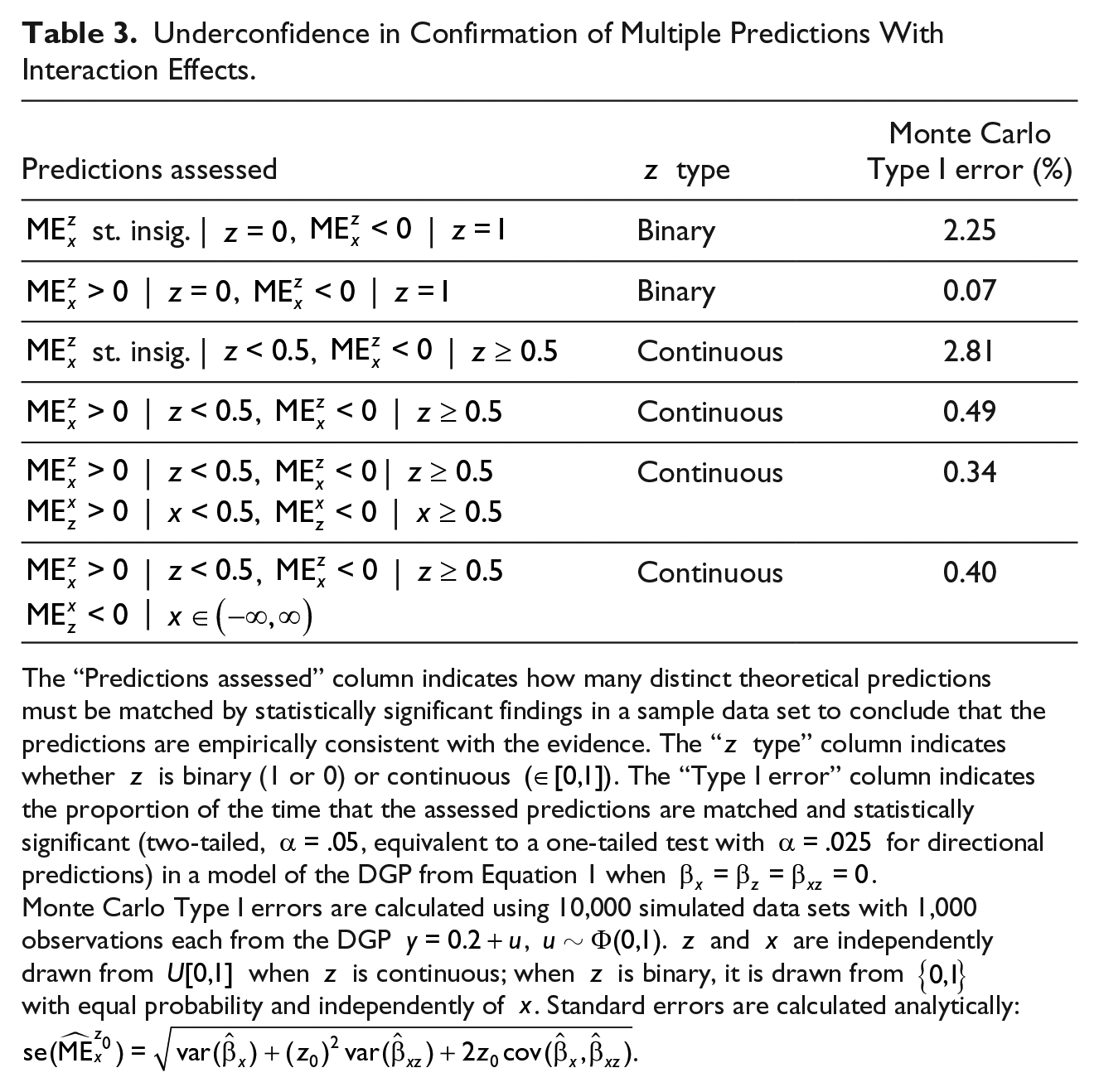
The underconfidence problem can be more or less severe (compared with the dichotomous case) when $z$ is continuous, depending on the pattern of predictions being tested. To determine the false positive rate when $z$ is continuous, we ran the Monte Carlo simulation from Table 1 under a default expectation that all marginal effects were nonexistent $(β_{x} = β_{z} = β_{x z} = 0)$ and checked for statistically significant marginal effects that matched a specified pattern of theoretical predictions using a two-tailed test, $α = . 05$ . These results (along with simulations for binary $z$ for comparison) are shown in Table 3. All the simulated false positive rates are smaller than the 5% nominal $α$ , and all but one are smaller than the 2.5% one-tailed $α$ to which a directional prediction corresponds. The degree of the test’s underconfidence varies according to the pattern of predictions.

Table 3.

Underconfidence in Confirmation of Multiple Predictions With Interaction Effects.

Predictions assessed	$z$ type	Monte Carlo Type I error (%)
${ME}_{x}^{z}$ st. insig. \| $z = 0$ , ${ME}_{x}^{z} < 0$ \| $z = 1$	Binary	2.25

${ME}_{x}^{z} > 0$ \| $z = 0$ , ${ME}_{x}^{z} < 0$ \| $z = 1$	Binary	0.07

${ME}_{x}^{z}$ st. insig. \| $z < 0.5$ , ${ME}_{x}^{z} < 0$ \| $z \geq 0.5$	Continuous	2.81

${ME}_{x}^{z} > 0$ \| $z < 0.5$ , ${ME}_{x}^{z} < 0$ \| $z \geq 0.5$	Continuous	0.49

${ME}_{x}^{z} > 0$ \| $z < 0.5$ , ${ME}_{x}^{z} < 0$ \| $z \geq 0.5$	Continuous	0.34

${ME}_{z}^{x} > 0$ \| $x < 0.5$ , ${ME}_{z}^{x} < 0$ \| $x \geq 0.5$

${ME}_{x}^{z} > 0$ \| $z < 0.5$ , ${ME}_{x}^{z} < 0$ \| $z \geq 0.5$	Continuous	0.40
${ME}_{z}^{x} < 0$ \| $x \in (- \infty, \infty)$

The “Predictions assessed” column indicates how many distinct theoretical predictions must be matched by statistically significant findings in a sample data set to conclude that the predictions are empirically consistent with the evidence. The “ $z$ type” column indicates whether $z$ is binary (1 or 0) or continuous $(\in [0, 1])$ . The “Type I error” column indicates the proportion of the time that the assessed predictions are matched and statistically significant (two-tailed, $α = . 05$ , equivalent to a one-tailed test with $α = . 025$ for directional predictions) in a model of the DGP from Equation 1 when $β_{x} = β_{z} = β_{x z} = 0$ . Monte Carlo Type I errors are calculated using 10,000 simulated data sets with 1,000 observations each from the DGP $y = 0.2 + u$ , $u \sim Φ (0, 1)$ . $z$ and $x$ are independently drawn from $U [0, 1]$ when $z$ is continuous; when $z$ is binary, it is drawn from ${0, 1}$ with equal probability and independently of $x$ . Standard errors are calculated analytically: $se ({\hat{ME}}_{x}^{z_{0}}) = \sqrt{var ({\hat{β}}_{x}) + {(z_{0})}^{2} var ({\hat{β}}_{x z}) + 2 z_{0} cov ({\hat{β}}_{x}, {\hat{β}}_{x z})}$ .

Thorough Testing of Possible Hypotheses: Underconfidence or Overconfidence?

The tension between over- and underconfidence of empirical results is illustrated in a recent article by BGM (2012) in the Journal of Politics. In that article, BGM (2012) recommend thoroughly testing all of the possible marginal effects implied by a statistical model. For a model like Equation 1, that means looking not only at $\partial y / \partial x$ at different values of $z$ but also at $\partial y / \partial z$ at different values of $x$ . Their reasoning is that ignoring the interaction between $\partial y / \partial z$ and $x$ allows researchers to ignore implications of a theory that may be falsified by evidence:

. . . the failure to make additional predictions about how the effect of $z$ varies with the value of $x$ , and to evaluate them with a second marginal effect plot, means that scholars often ignore evidence that can be extremely valuable for testing their theory. As a result, they either understate or, more worryingly, overstate the support for their theories.

If BGM are describing holistic testing of a particular theory with a large number of predictions, then we believe that our analysis tends to support their argument. As we show above, making multiple predictions about $\partial y / \partial x$ at different values of $z$ lowers the chance of a false positive under the standard hypothesis testing regime. The false positive rate is even lower if we holistically test a theory using multiple predictions about both $\partial y / \partial x$ and $\partial y / \partial z$ .

However, it is vital to note that following BGM’s suggestion will also make it more likely that at least one marginal effect will appear as statistically significant by chance alone. The reason for this is relatively straightforward: Testing a larger number of hypotheses means multiplying the risk of a single false discovery. In short, we contend that BGM are correct when testing a single theory by examining its multiple predictions as a whole, but caution that analyses that report any statistically significant findings separately could be made much more susceptible to false positives by this procedure.

What Now? Determining and Controlling the False Positive Rate for Tests of Interaction

The goal of this article is evolutionary, not revolutionary. We do not argue for a fundamental change in the way that we test hypotheses about marginal effects estimated in an interaction model—namely, by calculating estimates and CIs, and graphically assessing them—but we do believe that there is room to improve the interpretation of these tests. Specifically, we believe that the CIs that researchers report should reflect an intentional choice. We suggest three best practices to help political scientists achieve this goal.

Suggestion 1: Do Not Condition Inference on the Interaction Term, as It Does Not Solve the Multiple Comparison Problem

A researcher’s first inclination might be to fight the possibility of overconfidence by conditioning inference on the statistical significance of the interaction term, that is, for the case when $z$ is binary:

If ${\hat{β}}_{x z}$ is statistically significant: calculate ${\hat{ME}}_{x}^{0} = {\hat{β}}_{x}$ and ${\hat{ME}}_{x}^{1} = {\hat{β}}_{x} + {\hat{β}}_{x z}$ and interpret the statistical significance of each effect using the relevant 95% CI.

If ${\hat{β}}_{x z}$ is not statistically significant: drop $x z$ from the model, reestimate the model, calculate ${\hat{ME}}_{x}^{0} = {\hat{ME}}_{x}^{1} = {\hat{β}'}_{x}$ , and base acceptance or rejection of the null (that ${ME}_{x} = 0$ ) on the statistical significance of ${\hat{β}'}_{x}$

Braumoeller (2004, p. 814), one of the foundational pieces in the political science literature concerning the analysis of interacted relationships, uses this procedure in reanalyzing work originally published by Schultz (1999). However, this procedure results in an excess of false positives for ${\hat{ME}}_{x}$ . The reason is that a multiple comparison problem remains: The procedure allows two chances to conclude that $\partial y / \partial x \neq 0$ , one for a model that includes $x z$ and one for a model that does not.

Monte Carlo simulations reveal that the overconfidence problem with this procedure is substantively meaningful. We repeated the analysis of Table 1 with a binary $z \in {0, 1}$ under the null hypothesis, that $(\partial y / \partial x | z_{0}) = 0$ for all $z$ , conditioning inference on the statistical significance of the interaction term. This procedure results in a $8.17 %$ false positive rate when $α = . 05$ (two-tailed); the false positive rate is $9.60 %$ when $z$ is continuous.¹⁵ This is less overconfident than the Brambor et al. (2006) procedure using ${\hat{ME}}_{x}$ only, which resulted in ≈ $10 %$ false positive rates, but still larger than the advertised $α$ value. Therefore, we cannot recommend this practice as a way of correcting the overconfidence problem.

Suggestion 2: Use Tests Designed to Minimize False Discoveries and Maximize Power

In cases where a researcher believes that the over- or underconfidence of traditional hypothesis test procedures may be decisive to a result (i.e., when results are at the margin of some threshold for statistical significance), he or she can use an alternative test procedure to control the probability of a false positive (when overconfidence is a potential problem) or false disconfirmation of a theory that makes multiple predictions (when underconfidence is the relevant threat). We describe two separate test procedures, depending on whether the researcher believes overconfidence or underconfidence to be the likely problem. In this section, we will discuss each procedure in turn. In brief, for overconfidence, we recommend adapting the Benjamini and Hochberg (1995) procedure to control the FDR. For underconfidence, we suggest finding a critical $t$ statistic that produces a specified joint false positive rate using a nonparametric bootstrapping technique. Both of these procedures can be implemented using our R library, interactionTest .

Overconfidence corrections for estimated marginal effects

When a multiple comparison problem creates the danger of excess false discoveries, the literature supports two broad approaches to the problem. The first approach involves controlling the FDR, or the number of rejected null hypotheses that are false as a proportion of the total number of statistically significant results (Benjamini & Hochberg, 1995, pp. 291-292). In the context of testing the statistical significance of ${\hat{ME}}_{x}^{z}$ at multiple values of $z$ , the FDR is the proportion of statistically significant values of ${\hat{ME}}_{x}^{z}$ for which the null is actually true (i.e., ${ME}_{x}^{z} = 0$ ) in repeated tests. The second approach involves controlling the FWER, or the proportion of the time that a set of multiple comparisons (a “family” of hypothesis tests) will produce at least one false rejection of the null hypothesis (Abdi, 2007, pp. 2-4). For testing ${\hat{ME}}_{x}^{z}$ at multiple values of $z$ , the FWER is the proportion of the time (in repeated tests) in which at least one ${\hat{ME}}_{x}^{z}$ is statistically significant when the true ${ME}_{x}^{z} = 0$ . In general, a test that sets the FWER at some value is a more conservative procedure than a test that limits the FDR to the same value: A single rejection of any hypothesis where the null is true in a set of multiple comparisons raises the FWER, whereas the FDR allows a fixed level of false positives as a proportion of all statistically significant results. Consequently, procedures that control the FWER tend to be less powerful than those which control the FDR (Benjamini & Hochberg, 1995, p. 290).

A researcher can control the FDR for interacted relationships by adapting the procedure of Benjamini and Hochberg (1995, pp. 293-294; see also Spahn & Franco, 2015). For a categorical interaction variable $z$ with $m$ categories, their procedure suggests that the researcher should rank order each of the $p$ values, $p_{k}$ for $k \in {1 \dots m}$ ; $p_{1}$ is the smallest $p$ value and $p_{m}$ is the largest, with $k$ the rank index. Then, find the largest rank, $k = k^{⋆}$ , that satisfies $p_{k} < α (k / m)$ . The researcher then rejects the null hypothesis for all ${\hat{ME}}_{x}^{z_{j}}$ from $j = 1 \dots k^{⋆}$ at level $α$ ; this procedure ensures that the FDR is no larger than $α$ , though it can (in some cases) be smaller (see Theorem 1 in Benjamini & Hochberg, 1995).¹⁶ To visually depict which marginal effects are statistically significant, a researcher can use the critical $t$ statistic $t^{⋆}$ corresponding to $α (k^{⋆} / m)$ when constructing a 95% CI using $\hat{β} \pm t^{⋆} \times se ({\hat{ME}}_{x}^{z_{0}})$ at all values of $z_{0}$ . Note that this procedure also imposes a weak limit on the FWER: When all null hypotheses are true, that is, $(\partial y / \partial x | z = z_{0}) = 0$ for all values of $z_{0}$ , the FDR is equivalent to the FWER (Benjamini & Hochberg, 1995, p. 291).

Put another way, this procedure orders the $p$ values for all relevant values of $z$ and determines how many rejections of the null hypothesis can be made such that all $p$ values for the rejected hypotheses are less than the value of $α$ multiplied by $k^{⋆} / m$ . The $1 / m$ multiplier is a Bonferroni-type adjustment for multiple comparisons; this multiplier “deflates” $α$ to account for the joint probability of at least one false positive when m-many tests are conducted (Benjamini & Hochberg, 1995, p. 293). The innovation of Benjamini and Hochberg (1995) is to shift the statistic of interest to the proportion of rejected null hypotheses for which the null is true (instead of the probability of at least one rejection). This allows us to throw out highly statistically insignificant results from consideration in declining order of $p$ value, starting with $k = m$ , until we find $k^{⋆}$ . As each subsequent $p$ value is discarded and $k$ gets smaller, the size target $(α (k / m))$ to which all remaining $p$ values are compared also gets smaller. The process stops when all $p$ values are less than the deflated size target, $α (k^{⋆} / m)$ , which is then used to find a critical $t$ statistic. This critical $t$ statistic, $t^{⋆}$ , can then be used to construct marginal effects plots with CIs visually similar to those of Brambor et al. (2006); if a researcher uses these CIs to test multiple hypotheses, at most $α$ proportion of the rejected null hypotheses will be false. If $k^{⋆} = 1$ , the Bonferroni and Benjamini–Hochberg deflation factors are identical. The procedure to find an appropriate FDR-controlling $t^{⋆}$ for marginal effects calculated from an interaction model is included as a part of the new interactionTest R library that we developed for this article.

For controlling the FWER, Kam and Franzese (2007, pp. 43-51) recommend conducting a joint $F$ test to determine whether ${\hat{ME}}_{x}^{z}$ ≠ 0 for any value of $z$ when interaction between $x$ and $z$ (or other variables) is suspected. For a simple linear DGP with two variables of interest, this means running two models:

$\hat{y} = {\hat{β}}_{0} + {\hat{β}}_{x} x + {\hat{β}}_{z} z + {\hat{β}}_{x z} x z,$

$\hat{y} = {\hat{β}}_{0} + {\hat{β}}_{z} z .$

Then, the researcher can use an $F$ test to see whether the restrictions of Model 2 can be rejected by the data. If so, the researcher can proceed to construct, plot, and interpret ${\hat{ME}}_{x}^{z}$ using the procedure described in Brambor et al. (2006).¹⁷

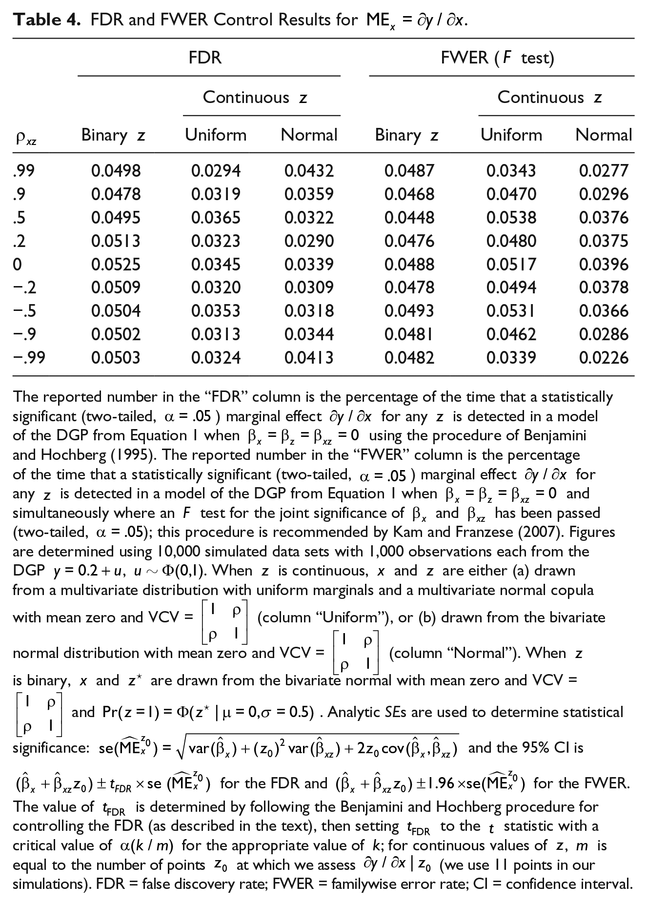
We used both of these procedures on the simulated data from Table 2; in each case, we set the target false positive rate (FDR or FWER) of the procedure to $. 05$ , two-tailed. The results are shown in Table 4. Because all the null hypotheses are true in the simulated data set (i.e., ${\hat{ME}}_{x}^{z_{0}} = 0$ for all $z_{0}$ ), both the procedures should yield roughly equivalent results (because the FDR in this case is equivalent to the FWER). Indeed, as the table indicates, both procedures are effective at limiting false rejections of the null to a probability of $≲ 5 %$ .

Table 4.

FDR and FWER Control Results for ${ME}_{x} = \partial y / \partial x$ .

$ρ_{x z}$	FDR			FWER ( $F$ test)
		Continuous $z$			Continuous
	Binary $z$	Uniform	Normal	Binary $z$	Uniform	Normal
.99	0.0498	0.0294	0.0432	0.0487	0.0343	0.0277
.9	0.0478	0.0319	0.0359	0.0468	0.0470	0.0296
.5	0.0495	0.0365	0.0322	0.0448	0.0538	0.0376
.2	0.0513	0.0323	0.0290	0.0476	0.0480	0.0375
0	0.0525	0.0345	0.0339	0.0488	0.0517	0.0396
−.2	0.0509	0.0320	0.0309	0.0478	0.0494	0.0378
−.5	0.0504	0.0353	0.0318	0.0493	0.0531	0.0366
−.9	0.0502	0.0313	0.0344	0.0481	0.0462	0.0286
−.99	0.0503	0.0324	0.0413	0.0482	0.0339	0.0226

The reported number in the “FDR” column is the percentage of the time that a statistically significant (two-tailed, $α = . 05$ ) marginal effect $\partial y / \partial x$ for any $z$ is detected in a model of the DGP from Equation 1 when $β_{x} = β_{z} = β_{x z} = 0$ using the procedure of Benjamini and Hochberg (1995). The reported number in the “FWER” column is the percentage of the time that a statistically significant (two-tailed, $α = . 05$ ) marginal effect $\partial y / \partial x$ for any $z$ is detected in a model of the DGP from Equation 1 when $β_{x} = β_{z} = β_{x z} = 0$ and simultaneously where an $F$ test for the joint significance of $β_{x}$ and $β_{x z}$ has been passed (two-tailed, $α = . 05$ ); this procedure is recommended by Kam and Franzese (2007). Figures are determined using 10,000 simulated data sets with 1,000 observations each from the DGP $y = 0.2 + u$ , $u \sim Φ (0, 1)$ . When $z$ is continuous, $x$ and $z$ are either (a) drawn from a multivariate distribution with uniform marginals and a multivariate normal copula with mean zero and VCV = $[\begin{matrix} 1 & ρ \\ ρ & 1 \end{matrix}]$ (column “Uniform”), or (b) drawn from the bivariate normal distribution with mean zero and VCV = $[\begin{matrix} 1 & ρ \\ ρ & 1 \end{matrix}]$ (column “Normal”). When $z$ is binary, $x$ and $z^{⋆}$ are drawn from the bivariate normal with mean zero and VCV = $[\begin{matrix} 1 & ρ \\ ρ & 1 \end{matrix}]$ and $\Pr (z = 1) = Φ (z^{⋆} | μ = 0, σ = 0.5)$ . Analytic SEs are used to determine statistical significance: $se ({\hat{ME}}_{x}^{z_{0}}) = \sqrt{var ({\hat{β}}_{x}) + {(z_{0})}^{2} var ({\hat{β}}_{x z}) + 2 z_{0} cov ({\hat{β}}_{x}, {\hat{β}}_{x z})}$ and the 95% CI is $({\hat{β}}_{x} + {\hat{β}}_{x z} z_{0}) \pm t_{F D R} \times se ({\hat{ME}}_{x}^{z_{0}})$ for the FDR and $({\hat{β}}_{x} + {\hat{β}}_{x z} z_{0}) \pm 1.96 \times se ({\hat{ME}}_{x}^{z_{0}})$ for the FWER. The value of $t_{FDR}$ is determined by following the Benjamini and Hochberg procedure for controlling the FDR (as described in the text), then setting $t_{FDR}$ to the $t$ statistic with a critical value of $α (k / m)$ for the appropriate value of $k$ ; for continuous values of $z$ , $m$ is equal to the number of points $z_{0}$ at which we assess $\partial y / \partial x | z_{0}$ (we use 11 points in our simulations). FDR = false discovery rate; FWER = familywise error rate; CI = confidence interval.

Underconfidence corrections for estimated marginal effects

As noted above, the Brambor et al. (2006) procedure is underconfident whenever a researcher is trying to conduct a conjoint test of multiple interaction relationships predicted by a preexisting theory. Consequently, the appropriate critical $t$ value to set a 5% probability of falsely rejecting the null of this conjoint test when examining CIs is not the typical $t^{⋆} = 1.96$ (for $n \to \infty$ ). Instead, we suggest a nonparametric bootstrapping approach to hypothesis testing that chooses the appropriate critical $t$ .

The intuition behind our approach is simple: Using simulation, determine a critical $t^{⋆}$ statistic that will produce joint confirmation of all a theory’s marginal effect predictions $α$ proportion of the time when in fact all the marginal effects are zero. If we use this $t^{⋆}$ to construct CIs for marginal effects plots (using the ordinary formula for CIs and the analytically calculated standard errors from the original model) in the style of Brambor et al. (2006), we will be able to simply look at these plots to determine whether the theory’s marginal effects predictions are supported by evidence with the reassurance that this procedure will yield a false positive empirical confirmation of the predictions at most $100 \times α$ percent of the time when all marginal effects are zero.

The specific step-by-step details of our procedure are described in an appendix; however, we provide R code to implement this procedure for generalized linear models as a part of our interactionTest R library. This R library leverages the boot package (Canty & Ripley, 2017) to perform ordinary bootstrap resampling of the target data set. The bootstrapping process can be computationally intensive and lengthy; to speed up performance, the boot package can interface with the snow library (Tierney, Rossini, Li, & Sevcikova, 2015) to use parallel processing with multiple central processing unit (CPU) cores for faster computation. Our library documentation provides an example of using parallel processing through snow.

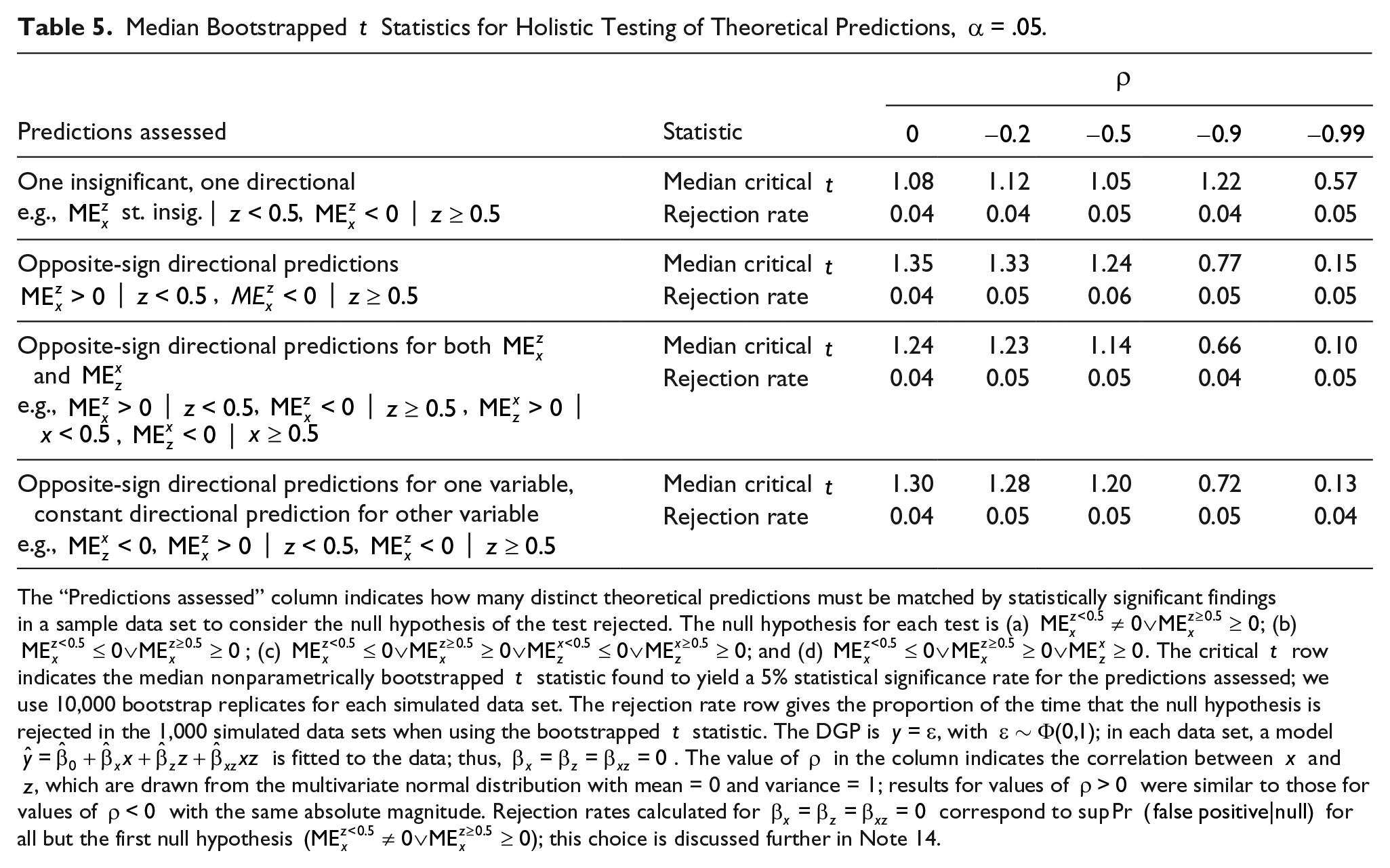
We tested the effectiveness of the nonparametric bootstrapping procedure in 1,000 simulated data sets with $N = 1, 000$ observations when all marginal effects are zero for four different patterns of theoretical predictions; these theoretical predictions, the rejection rate of the bootstrapping procedure, and the median critical $t$ found by the bootstrapping procedure are shown in Table 5. We also show the proportion of the time that using the critical $t$ statistic generated from the bootstrapping procedure results in a rejection of the null hypothesis of the corresponding hypothesis test.¹⁸ The table shows that different patterns of predictions have a different probability of appearing by chance, which in turn necessitates a different critical $t$ statistic; furthermore, this critical $t$ changes according to the correlation between $x$ and $z$ . Indeed, some patterns are so unlikely under some conditions that nearly any estimates matching the pattern are not ascribable to chance, regardless of their uncertainty. The procedure results in false positive rates that match the nominal 5% rate targeted by the test.

Table 5.

Median Bootstrapped $t$ Statistics for Holistic Testing of Theoretical Predictions, $α = . 05$ .

Predictions assessed	Statistic	$ρ$
Predictions assessed	Statistic	$0$	$- 0.2$	$- 0.5$	$- 0.9$	$- 0.99$
One insignificant, one directionale.g., ${ME}_{x}^{z}$ st. insig. \| $z < 0.5$ , ${ME}_{x}^{z} < 0$ \| $z \geq 0.5$	Median critical $t$	1.08	1.12	1.05	1.22	0.57
	Rejection rate	0.04	0.04	0.05	0.04	0.05

Opposite-sign directional predictions ${ME}_{x}^{z} > 0$ \| $z < 0.5$ , $M E_{x}^{z} < 0$ \| $z \geq 0.5$	Median critical $t$	1.35	1.33	1.24	0.77	0.15
	Rejection rate	0.04	0.05	0.06	0.05	0.05

Opposite-sign directional predictions for both ${ME}_{x}^{z}$ and ${ME}_{z}^{x}$ e.g., ${ME}_{x}^{z} > 0$ \| $z < 0.5$ , ${ME}_{x}^{z} < 0$ \| $z \geq 0.5$ , ${ME}_{z}^{x} > 0$ \| $x < 0.5$ , ${ME}_{z}^{x} < 0$ \| $x \geq 0.5$	Median critical $t$	1.24	1.23	1.14	0.66	0.10
	Rejection rate	0.04	0.05	0.05	0.04	0.05

Opposite-sign directional predictions for one variable, constant directional prediction for other variablee.g., ${ME}_{z}^{x} < 0$ , ${ME}_{x}^{z} > 0$ \| $z < 0.5$ , ${ME}_{x}^{z} < 0$ \| $z \geq 0.5$	Median critical $t$	1.30	1.28	1.20	0.72	0.13
	Rejection rate	0.04	0.05	0.05	0.05	0.04

The “Predictions assessed” column indicates how many distinct theoretical predictions must be matched by statistically significant findings in a sample data set to consider the null hypothesis of the test rejected. The null hypothesis for each test is (a) ${ME}_{x}^{z < 0.5} \neq 0 \lor {ME}_{x}^{z \geq 0.5} \geq 0$ ; (b) ${ME}_{x}^{z < 0.5} \leq 0 \lor {ME}_{x}^{z \geq 0.5} \geq 0$ ; (c) ${ME}_{x}^{z < 0.5} \leq 0 \lor {ME}_{x}^{z \geq 0.5} \geq 0 \lor {ME}_{z}^{x < 0.5} \leq 0 \lor {ME}_{z}^{x \geq 0.5} \geq 0$ ; and (d) ${ME}_{x}^{z < 0.5} \leq 0 \lor {ME}_{x}^{z \geq 0.5} \geq 0 \lor {ME}_{z}^{x} \geq 0$ . The critical $t$ row indicates the median nonparametrically bootstrapped $t$ statistic found to yield a 5% statistical significance rate for the predictions assessed; we use 10,000 bootstrap replicates for each simulated data set. The rejection rate row gives the proportion of the time that the null hypothesis is rejected in the 1,000 simulated data sets when using the bootstrapped $t$ statistic. The DGP is $y = ε$ , with $ε \sim Φ (0, 1)$ ; in each data set, a model $\hat{y} = {\hat{β}}_{0} + {\hat{β}}_{x} x + {\hat{β}}_{z} z + {\hat{β}}_{x z} x z$ is fitted to the data; thus, $β_{x} = β_{z} = β_{x z} = 0$ . The value of $ρ$ in the column indicates the correlation between $x$ and $z$ , which are drawn from the multivariate normal distribution with mean = 0 and variance = 1; results for values of $ρ > 0$ were similar to those for values of $ρ < 0$ with the same absolute magnitude. Rejection rates calculated for $β_{x} = β_{z} = β_{x z} = 0$ correspond to sup Pr $(false positive | null)$ for all but the first null hypothesis $({ME}_{x}^{z < 0.5} \neq 0 \lor {ME}_{x}^{z \geq 0.5} \geq 0)$ ; this choice is discussed further in Note 14.

Suggestion 3: Specify Theories With Multiple Predictions in Advance and Use Bootstrapped Critical $t$ Statistics to Maximize Empirical Power

Correcting for the overconfidence of conventional pointwise 95% CIs when performing interaction tests does come at a price: When the null hypothesis is false, the sensitivity of the corrected test is necessarily less than that of an uncorrected test. This trade-off is fundamental to all hypothesis tests and not specific to the analysis of interaction: Lowering the size of the test, as we do by setting the FDR or FWER to 0.05, weakens the power of a test to detect relationships when they are actually there. On the contrary, correcting for underconfidence when simultaneously testing multiple theoretical predictions makes (jointly) confirming these predictions easier.

As a result, we suggest that researchers generate and simultaneously test multiple empirical predictions whenever possible to maximize the power of their empirical test. For interaction terms, this means

predicting the existence and direction of a marginal effect for multiple values of the intervening variable, and/or

predicting the existence and direction of the marginal effect of both constituent variables in an interaction.

This suggestion is subject to two important caveats. First, researchers must use bootstrapped-derived critical $t$ statistics (as in Table 3) to reap the benefit of a more powerful test; simply testing each prediction separately using pointwise CIs (as suggested by BGM, 2012) would result in diminished power as a result of using overly conservative tests (as shown in the previous section of this article). Second, the predictions must be made before consulting sample data in order for the lowered confidence thresholds to apply. The lowered significance thresholds are predicated on the likelihood of simultaneous appearance of a particular combination of results when all marginal effects are zero, not on the joint likelihood of many possible combinations of results.

Application: “Rehabilitating Duverger’s Law”

After publishing their recommendations for the proper hypothesis test for a marginal effect in the linear model with interaction terms, Clark and Golder (2006) went on to apply this advice in a Comparative Political Studies article examining the relationship between the number of political parties in a polity and the electoral institutions of that polity. Their reassessment of Duverger’s Law applies the spirit behind the simple relationship between seats and parties predicted by Duverger to specify a microfoundational mechanism by which institutions and sociological factors are linked to political party viability. Based on a reanalysis of their results with the methods that we propose, we believe that some of the authors’ conclusions are more uncertain than originally believed.

Clark and Golder (2006) expect that ethnic heterogeneity (a social pressure for political fragmentation) will have a positive relationship with the number of parties that gets larger as average district magnitude increases. Specifically, they propose,

Hypothesis 4: Social heterogeneity increases the number of electoral parties only when the district magnitude is sufficiently large. (Clark & Golder, 2006, p. 694)

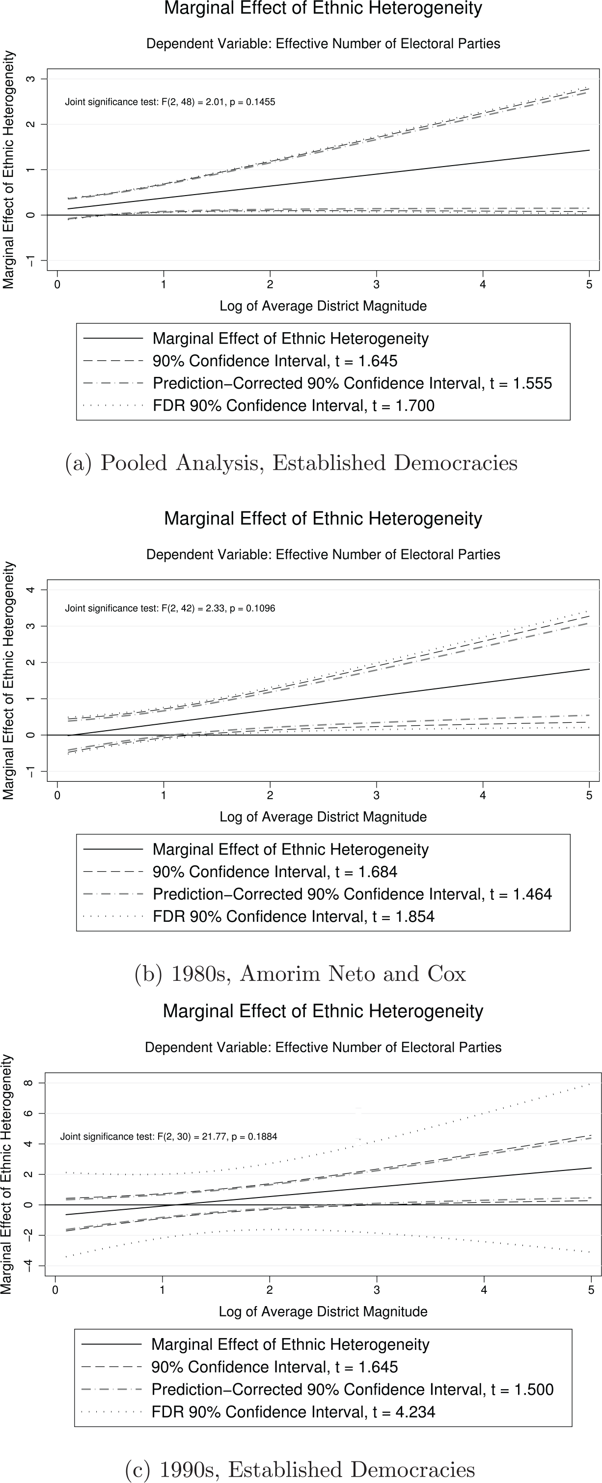
We interpret their hypothesis to mean that the marginal effect of ethnic heterogeneity on the number of electoral parties should be positive when district magnitude is large, and statistically insignificant when district magnitude is small. To test for the presence of this relationship, the authors construct plots depicting the estimated marginal effect of ethnic heterogeneity on number of parties at different levels of district magnitude for a pooled sample of developed democracies, for 1980s cross-sectional data (using the data from Amorim Neto & Cox, 2007), and for established democracies in the 1990s. In all three samples, they find that ethnic heterogeneity has a positive and statistically significant effect on the number of parties once district magnitude becomes sufficiently large.

Figure 2 displays our replication of the marginal effects plots from Clark and Golder (2006). We show three different CIs: (a) the authors’ 90% CIs (using a conventional $t$ test); (b) a 90% CI with a nonparametrically bootstrapped critical $t$ designed to set the false positive rate at 5% for the pattern of predictions where ${ME}_{x}^{z < 2.5}$ is statistically insignificant and ${ME}_{x}^{z \geq 2.5} > 0$ (where $x$ is ethnic heterogeneity and $z$ is log average district magnitude), which we call the “prediction-corrected” CI; and (c) a 90% CI constructed using the FDR-controlling procedure of Benjamini and Hochberg (1995). We also calculate and show the results of a joint $F$ test as prescribed by Kam and Franzese (2007).

Figure 2.

Marginal effect of electoral parties (Clark & Golder, 2006, Figure 1), with original and prediction- and discovery-corrected confidence intervals.

None of the joint $F$ tests for the statistical significance of the marginal effect of ethnic heterogeneity yield one-tailed $p$ values less than .1. In addition, FDR-controlling 90% CIs include zero across the entire range of district magnitude for the sample of established democracies in the 1990s. However, in the other two samples, the coverage of the 90% FDR CIs confirms the authors’ original results, albeit with somewhat greater uncertainty. In addition, the authors’ original findings are statistically significant and consistent with their pattern of theoretical predictions when we employ the prediction-corrected 90% CIs.

In summary, our analysis indicates that the authors’ claims are most strongly supported by a combination of the empirical information they collect with the prior theoretical prediction of an unlikely pattern of results. Their results cannot be supported by a procedure that sets the FWER at 90% and are only partially supported by a procedure that sets the FDR at 90%. We believe that this reinterpretation of the authors’ findings is important for readers to understand in order for them to grasp the strength of the results and the assumptions upon which these results are based.

Conclusion

The main argument of this study is that, when it comes to the contextually conditional (interactive) relationships that have motivated a great deal of recent research, the Brambor et al. (2006) procedure for testing for a relationship between $x$ and $y$ at different values of $z$ does not effectively control the probability of a false positive finding. The probability of at least one relationship being statistically significant is higher than one expects because the structure of interaction models divides a data set into multiple subsets defined by $z$ , each of which has a chance of showing evidence for a relationship between $x$ and $y$ when none really exists. On the contrary, the possibility of simultaneously confirming multiple theoretical predictions by chance alone can be quite small because this requires a large number of individually unlikely events to occur together, making the combination of these events collectively even more unlikely. The consequence is that false positive rates may be considerably higher or lower than researchers believe when they conduct their tests. A further consequence is that researchers using the Brambor, Clark, and Golder procedure are implicitly applying inconsistent standards to assess whether evidence tends to support or undermine a theory when that theory makes multiple empirical predictions.

Fortunately, we believe that specifying a consistent false positive rate for interactive relationships is a comparatively simple matter of following a few rules of thumb:

Do not condition inference about marginal effects on the statistical significance of the product term;

If a relationship is close to statistical significance under conventional tests, use procedures that control the overall FDR and/or FWER, such as the sequential test procedure of Benjamini and Hochberg (1995) or the joint $F$ test recommended by Kam and Franzese (2007); and

If possible, generate multiple hypotheses about contextual relationships before consulting the sample data and test them as a group using a nonparametric bootstrapping procedure to generate the appropriate critical $t$ value, because it maximizes the power of the study.

Our new interactionTest software package for R makes it easy for applied researchers to control the false positive rate when they create marginal effects plots in the mode of Clark and Golder (2006), even in the complex case where multiple theoretical predictions present a threat of underconfident statistical hypothesis tests.

None of these recommendations constitutes a fundamental revision to the way we conceptualize or depict conditional relationships. Rather, they allow us to ensure that evidence we collect is compared with a counterfactual world in a controlled fashion and consistent with the hypothesis tests that we perform in other situations. All of our recommendations can be implemented in standard statistical packages; we hope that researchers will keep them in mind when embarking on future work involving the assessment of conditional marginal effects.

Footnotes

Appendix

Acknowledgements

Nathan Edwards provided research assistance while writing this paper, for which we are grateful. We received helpful feedback on earlier versions of this paper from Kyle Beardsley, William D. Berry, Christopher Gandrud, Tom Pepinsky, Meg Shannon, anonymous reviewers, and participants in our panel at the 2012 Annual Meeting of the Society for Political Methodology and in a 2012 presentation in the Emory Political Science Colloquium Series.

Declaration of Conflicting Interests

The authors declared no potential conflicts of interest with respect to the research, authorship, and/or publication of this article.

Funding

The authors received no financial support for the research, authorship, and/or publication of this article.

Supplemental Material

Supplementary material for this article is available online at the CPS website .

Notes

Author Biographies

Justin Esarey is an associate professor of Political Science at Rice University who specializes in political methodology. His areas of expertise include detecting and presenting context-specific relationships, model specification and sensitivity, and using technology to make methodological resources available to the scholarly public.

Jane Lawrence Sumner is an assistant professor of Political Science at the University of Minnesota, Twin Cities. She is interested in the accessibility of applied methods, data availability and quality, and measurement. She also studies international political economy, with a focus on the politics of multinational production and non-state service delivery.

References

Abdi

(2007). The Bonferonni and Sidak corrections for multiple comparisons. In Salkind

(Ed.), Encyclopedia of measurement and statistics (pp. 103-106). Thousand Oaks, CA: Sage.

Norton

E. C.

(2003). Interaction terms in logit and probit models. Economics Letters, 80, 123-129.

Amorim Neto

Cox

G. W.

(2007). Electoral institutions, cleavage structures, and the number of parties. American Journal of Political Science, 41, 149-174.

Benjamini

Hochberg

(1995). Controlling the false discovery rate: A practical and powerful approach to multiple testing. Journal of the Royal Statistical Society. Series B (Methodological), 57, 289-300.

Berry

W. D.

DeMeritt

J. H. R.

Esarey

(2010). Testing for interaction in binary logit and probit models: Is a product term essential? American Journal of Political Science, 54, 248-266.

Berry

W. D.

Golder

Milton

(2012). Improving tests of theories positing interaction. Journal of Politics, 74, 653-671.

Brambor

Clark

W. R.

Golder

(2006). Understanding interaction models: Improving empirical analyses. Political Analysis, 14, 63-82.

Braumoeller

B. F.

(2004). Hypothesis testing and multiplicative interaction terms. International Organization, 58, 807-820.

Canty

Ripley

(2017). boot: Bootstrap R (S-Plus) Functions (R Package Version 1.3-19).

10.

Clark

W. R.

Golder

(2006). Rehabilitating Duverger’s theory. Comparative Political Studies, 39, 679-708.

11.

Hochberg

(1988). A sharper Bonferroni procedure for multiple tests of significance. Biometrika, 75, 800-802.

12.

Holm

(1979). A simple sequentially rejective multiple test procedure. Scandinavian Journal of Statistics, 6, 65-70.

13.

Kam

C. D.

Franzese

R. J.

(2007). Modeling and interpreting interactive hypotheses in regression analysis. Ann Arbor: University of Michigan Press.

14.

King

Tomz

Wittenberg

(2000). Making the most of statistical analyses: Improving interpretation and presentation. American Journal of Political Science, 44, 347-361.

15.

Kutner

Nachtsheim

C. J.

Neter

(2004). Applied linear statistical models (4th ed.). New York, NY: McGraw-Hill.

16.

Lehmann

E. L.

(1957a). A theory of some multiple decision problems, I. The Annals of Mathematical Statistics, 28, 1-25.

17.

Lehmann

E. L.

(1957b). A theory of some multiple decision problems, II. The Annals of Mathematical Statistics, 28, 547-572.

18.

Rainey

(2014). Arguing for a negligible effect. American Journal of Political Science, 58, 1083-1091.

19.

R Core Team. (2017). R: A language and environment for statistical computing. Vienna, Austria: R Foundation for Statistical Computing. Available from https://www.R-project.org/

20.

Rom

D. M.

(1990). A sequentially rejective test procedure based on a modified Bonferroni inequality. Biometrika, 77, 663-665.

21.

Schultz

K. A.

(1999). Do democratic institutions constrain or inform? Contrasting two institutional perspectives on democracy and war. International Organization, 53, 233-266.

22.

Shaffer

J. P.

(1995). Multiple hypothesis testing. Annual Review of Psychology, 46, 561-584.

23.

Sidak

(1967). Rectangular confidence regions for the means of multivariate normal distributions. Journal of the American Statistical Association, 62, 626-633.

24.

Spahn

Franco

(2015). A false discovery framework for mitigating publication bias. Retrieved from https://wustl.app.box.com/s/7hrwt5qhi0gxsq6w34ri5cczsk3a6z75/file/119378926919

25.

Tierney

Rossini

A. J.

Sevcikova

(2015). Snow: Simple Network of Workstations (R Package Version 0.4-1). Retrieved from https://CRAN.R-project.org/package=snow

Supplementary Material

Please find the following supplemental material available below.

For Open Access articles published under a Creative Commons License, all supplemental material carries the same license as the article it is associated with.

For non-Open Access articles published, all supplemental material carries a non-exclusive license, and permission requests for re-use of supplemental material or any part of supplemental material shall be sent directly to the copyright owner as specified in the copyright notice associated with the article.

5.26 MB

0.00 MB

Marginal Effects in Interaction Models: Determining and Controlling the False Positive Rate

Abstract

Keywords

Introduction

Interaction Terms and the Multiple Comparison Problem

Interaction Terms Create a Multiple Comparison Problem: The Case of a Dichotomous Interaction Variable

Continuous Interaction Variables

Statistical Interdependence Between Marginal Effects Estimates

Underconfidence Is Possible for Conjoint Tests of Theoretical Predictions

Dichotomous Interaction Variable

Continuous Interaction Variable

Thorough Testing of Possible Hypotheses: Underconfidence or Overconfidence?

What Now? Determining and Controlling the False Positive Rate for Tests of Interaction

Suggestion 1: Do Not Condition Inference on the Interaction Term, as It Does Not Solve the Multiple Comparison Problem

Suggestion 2: Use Tests Designed to Minimize False Discoveries and Maximize Power

Overconfidence corrections for estimated marginal effects

Underconfidence corrections for estimated marginal effects

Suggestion 3: Specify Theories With Multiple Predictions in Advance and Use Bootstrapped Critical t Statistics to Maximize Empirical Power

Application: “Rehabilitating Duverger’s Law”

Conclusion

Footnotes

Appendix

Acknowledgements

Declaration of Conflicting Interests

Funding

Supplemental Material

Notes

Author Biographies

References

Supplementary Material

Suggestion 3: Specify Theories With Multiple Predictions in Advance and Use Bootstrapped Critical $t$ Statistics to Maximize Empirical Power