
Abstract
Much criminological research has used longitudinal data to assess change in offending over time. An important feature of some data sources is that they contain cross-sections of different aged individuals followed over successive time periods, thereby potentially conflating age and time. This article compares the substantive conclusions about the relationship between age and offending based on trajectory modeling analyses by time-of-assessment versus age-at-assessment. Analyses of a large sample of serious youthful offenders followed for 7 years consisted of estimation of group-based offending trajectories and multinomial logistic regressions examining how risk/protective factors distinguished between offending trajectories. Findings revealed that concordance using measurement approaches was strong at relatively high and low levels of antisocial behavior, with greater ambiguity between these two offending extremes. The relation of risk/protective factors to various trajectories was substantively similar across measurement approaches.
Introduction
Critics notwithstanding (Gottfredson & Hirschi, 1990), longitudinal studies come with the promise of generating unique insights into longitudinal patterns of criminal activity over the life course (Blumstein et al., 1986; Farrington, Ohlin, & Wilson, 1986; Piquero, Farrington, & Blumstein, 2003). Compared with cross-sectional study designs, longitudinal studies are able to track the onset, persistence, and desistance from crime; track the factors that promote and reduce criminal activity; and assess the more general relationship between continuity and change in offending. Thus, longitudinal studies provide a mechanism to study the relationship between age and crime over the life course.
However, the design and analysis of longitudinal data pose a number of challenges to researchers (Eggleston, Laub, & Sampson, 2004). Recently, these methodological and statistical challenges have increased as a result of the development and availability of longitudinal studies that contain a cross-section of different aged individuals at the baseline of measurement (i.e., a longitudinal overlapping cohort design). The concern for criminologists is that when modeling longitudinal changes in criminal behavior with age, different individuals may be at different points in their age–crime curves at the start of the observation window and then follow different age–crime paths across successive measurement points (Lauritsen, 1998)—This will also be true for victimization as an outcome. For example, many data sets have cross-sections of ages at the initial period of survey assessment such as the National Youth Survey (NYS, ages 11-17), the National Longitudinal Study of Adolescent Health (Add Health, Grades 7-12), and the National Longitudinal Survey of Youth–1997 (NLSY97, ages 12-16). Yet, dramatically different conclusions could be reached if an investigator decides to analyze data by age-at-assessment or by time-of-assessment. Given that many of these data sets are publicly available and have generated a large body of research, an examination of how modeling differences (i.e., age vs. time) impact study results is imperative. Above and beyond conclusions about the association between age and crime drawn from different modeling strategies, there is a need to consider whether substantive conclusions regarding the relationship of risk and protective factors to offending patterns may be different if the assessments are based on age-at-assessment or if they are based on time-of-assessment. This article explores this issue using longitudinal data from a large sample of serious youthful offenders from adolescence to early adulthood. 1
Two prior investigations are pertinent to the current study. First, Osgood, O’Malley, Bachman, and Johnston (1989) used data from the Monitoring the Future study, an annual survey of high school seniors, to study time and age trends in crime. Time trends (of constant aged respondents) were investigated from 1975 to 1985 using responses from the high school senior classes of 1976 through 1986, whereas age trends between ages 17 and 23 were analyzed using four waves of data from the follow-up portion, which includes a subsample of each senior class. Although Osgood et al. also examined arrest rates to assess how they matched up to the self-report data, we limit our review to their self-report findings. Several results are worthy of mention. First, regarding age trends, most illegal behavior decreased over time from ages 17 to 23, but aggravated assault peaked in the late teens/early 20s, whereas other types of antisocial behavior peaked earlier in adolescence. Second, analysis of time trends did not reveal as consistent a set of findings as the age trends did, although there was a noticeable finding in the time trend assault analysis, which showed an increase from 1975 to 1985. This result notwithstanding, the time trends were more erratic and thus summary conclusions were deemed premature, suggesting that analyses by age and time derive substantially different results.
In a second study, Lauritsen (1998) used data from the NYS, a prospective longitudinal study of more than 1,600 youths who were between ages 11 and 17 at the first wave of data collection (1976), to investigate changes in criminal activity throughout adolescence and into early adulthood. Focusing on four of the seven available age cohorts (11, 13, 15, or 17 years old at the time of the first wave of data collection), she examined the relation between age and several measures of delinquency/victimization (general delinquency, serious offending, and victimization) over a consecutive 5-year period (when participants were 15-21 years old), thereby “treating the NYS panel data as an accelerated longitudinal design with multiple age cohorts” (Lauristen, 1998, p. 129). These analyses produced several findings. First, with one exception (among the 11-year-old cohort), the average rate of change in general delinquency in the subsequent four panels was decreasing for the 13-, 15-, and 17-year-old cohorts. These findings suggest that the expected age–crime curve relationship was not observed for general delinquency when trajectories were estimated for age cohorts. Second, age-cohort analysis of serious offending and victimization was substantively similar to the general delinquency results. For serious offending, once again the slopes were negative, indicating decreasing involvement in serious offending over time for all but the 11-year-old cohort. For victimization, all the slopes for all age cohorts displayed significant decreases in victimization across successive waves. These results show that the general form of the cohort-specific age–crime curves in the NYS . . . are not as expected . . . [and that] regardless of whether the respondent was 13, 15, or 17 years old at the start of data collection, the average subject reported decreasing involvement in general delinquency, serious offending, and victimization in the subsequent four panels. (Lauristen, 1998, pp. 138-139)
Third, Lauritsen examined whether the NYS cohort data could be linked to study the age/crime relationship, that is, that a single developmental trajectory could describe involvement in crime from ages 11 to 21. To do so, she linked the age 11 and age 13 cohorts, the age 13 and age 15 cohorts, and the age 15 and age 17 cohorts, and examined how they related to general delinquency, serious offending, and victimization. Across several analyses, she found that while a general decline in crime from ages 15 to 21 could be inferred from linking the 15- and 17-year-old cohorts, the younger age cohorts could not be similarly linked. This suggests that methodological problems associated with longitudinal research designs may be more or less pronounced across different age youth, including issues surrounding potential testing effects or changes in content validity associated with the respondent’s age. 2
Current Study
Given that researchers may choose to model longitudinal data of criminal behavior by age, if developmental questions are of importance, or by time, if time-based implications are important such as time to reoffense or treatment implications, it is important to understand how the same data may generate concurrent or disparate findings and implications on the basis of statistical modeling by age or by time. The present study investigates how modeling data by (a) age-at-assessment or (b) time-of-assessment alters conclusions about the developmental patterns of antisocial behavior. Furthermore, the current article builds from previous work to test if the substantive conclusions about risk and protective factors vary based on whether analyses are conducted by age-at-assessment or time-of-assessment. Notably, this study addresses these important but unstudied questions in a unique sample of serious juvenile offenders, precisely the sample that would be expected to begin desisting from crime between adolescence and early adulthood. In addition, the present study models change in offending while controlling for time incarcerated (i.e., exposure time), which allows greater specificity with respect to the level of criminal offending across time, given one’s time to engage in criminal activity. Thus, the present study can evaluate the link between criminal offending across different analytic models (age vs. time) while accounting for time incarcerated.
Data
This article uses data from a subset of the participants enrolled in the Pathways to Desistance study, a longitudinal investigation of the transition from adolescence to young adulthood among serious adolescent offenders. The enrolled youth were at least 14 years old and below 18 years old at the time of their committing offense and were found guilty of a serious offense (predominantly felonies, with a few exceptions for some misdemeanor property offenses, sexual assault, or weapon offenses) in the juvenile or adult court systems in Maricopa County, Arizona, or Philadelphia County, Pennsylvania. A total of 1,354 adolescents are enrolled in the study, representing approximately 1 in 3 adolescents adjudicated on the enumerated charges in each locale during the recruitment period (November 2000 through January 2003). The baseline interview was conducted an average of 39.2 days (SD = 25.9) after participants’ adjudication (for those in the juvenile system) or their decertification (i.e., waiver) hearing in Philadelphia or an adult arraignment in Phoenix (if in the adult system). Youth were predominantly 14 to 18 years of age at the time of the baseline interview, with a mean age of 16.5 years. 3 Follow-up interviews were conducted every 6 months for the first 3 years of the study and annually thereafter through 7 years. The present analyses are limited to males because there were an insufficient number of females to analyze. Information regarding the rationale and overall design of the study can be found in Mulvey et al. (2004), whereas details regarding recruitment, a description of the full sample, and the study methodology are discussed in Schubert et al. (2004).
The full study sample comprises mainly non-White (41.4% African American, 33.5% Hispanic) males (86%), who were, on average, 14.9 years old at the age of their first petition, with an average of three petitions prior to the baseline interview. Retention of the sample has been excellent. For example, an average of 90% of the sample completed each follow-up assessment and 87% of the sample missed no more than three assessments across the 7-year follow-up period. The time-based trajectory models were based on the baseline interview (T0) and 10 follow-up assessments spaced either 6 or 12 months apart (i.e., baseline, 6 months, 12 months, 18 months, 24 months, 30 months, 36 months, 48 months, 60 months, 72 months, and 84 months) in line with the study design noted above. The shift to annual interviews in the later waves was a study design decision based on the desire to follow youth for a longer period of time within the constraints of available funding. The age-based trajectory models were based on the sample’s age at the interview time period. For this estimation procedure, we centered on age at the baseline interview, for a total number of self-reported-offending (SRO)–variety measures, explained subsequently, to include the baseline (T0) interview as well as 10 additional measures, for a total of 11 SRO-variety scores.
To create uniform time measurement for the age-based analyses, we combined data from the 6- to 36-month biannual follow-up interviews into yearlong intervals by counting the variety of endorsed self-reported offenses across the 6- and 12-month assessments, the 18- and 24-month assessments, and the 30- and 36-month assessments, respectively.
As a consequence of the measurement decisions for age vs. time analyses (i.e., combining data from the age-of-assessment outcomes into annual assessments), sample selection for the current analyses varied slightly based on whether analyses were conducted by age or by time. For the time-based trajectories, data were restricted to males (n = 1,170), and only participants with 70% data were included in the analysis (n = 1,051). For the age-based trajectories, the analyses were limited to 1,088 males in the sample who had completed at least 70% of the interviews administered during the 7-year study (n = 565 from Phoenix, n = 605 from Philadelphia; full male sample n = 1,170). 4
There is a small discrepancy between the sample sizes (n = 37) used to derive the age-based and time-based trajectories. For both approaches, individuals had to provide information from 70% of assessments. The time-based analyses used participants who had a partial assessment as long as it included valid data regarding antisocial behavior. Each follow-up interview contributed individually to the 70% threshold in this approach. The age-based analyses followed a similar strategy, except that when follow-up interviews were combined into yearlong intervals, a case was included as long as one or the other follow-up interviews included a valid report of antisocial behavior. This slightly different approach led to the sample size difference of 37 cases between the two trajectory analyses.
Self-Reported Variety of Offending
For purposes of this study, outcome data were obtained for a 7-year time period post baseline enrollment interview. At each interview, the SRO (Huizinga, Esbensen, & Weiher, 1991) was used to measure involvement in antisocial and illegal activities. Participants reported whether they had been involved in any of 22 aggressive or income-generating activities (e.g., “taken something from another person by force, using a weapon,” “used checks or credit cards illegally”; see appendix for a full list of items). In all, 2 of the 24 activities were added to the Pathways research battery after a large number of participants had completed either baseline or 6-month follow-up interviews. Although all 24 acts were examined for the vast majority of cases, the current analyses are based on summary scores that eliminate those 2 added items so that there is consistency across cases. At the baseline and 48-, 60-, 72-, and 84-month interviews, these 22 items were asked at each time point with the qualifying phrase, “In the past 12 months, have you . . . .” At the 6- through 36-month follow-up interviews, these questions were asked with the qualifying phrase, “In the past 6 months, have you . . . .”
In this study, SRO-variety scores are used and are calculated based on a count of the 22 different acts that an individual endorsed at each recall period. Specifically, a sum of the number of different types of crime that an individual endorsed in each recall period was calculated. Offending variety scores are a common method of examining offending and have several desirable features (Hindelang, Hirschi, & Weis, 1981; Moffitt, Caspi, Rutter, & Silva, 2001): (a) They capture involvement in multiple forms of crime so that trivial acts do not overweight the measure; (b) variety scores have better distributional properties for analyses than frequency scores (less skewness); (c) they predict future delinquency; (d) they show the extent of involvement in different crime types, which is a highly reliable predictor of future antisocial outcomes; (e) they are more accurate and reliable than frequency measures, especially with respect to recall errors; and (f) they are the preferred measure according to Hindelang et al.’s (1981) classic study on delinquency assessment. Prior analyses of antisocial behavior in this sample using SRO-variety scores show that common delinquency correlates relate to it as expected (Mulvey et al., 2010), that the SRO-variety and SRO-frequency measures are highly correlated (i.e., high frequency–high variety; Monahan & Piquero, 2009), that there is a strong correlation between self-reported and official records of offending (Brame, Fagan, Piquero, Schubert, & Steinberg, 2004), and that there is consistency of reporting across racial/ethnic groups (Knight, Little, Losoya, & Mulvey, 2004).
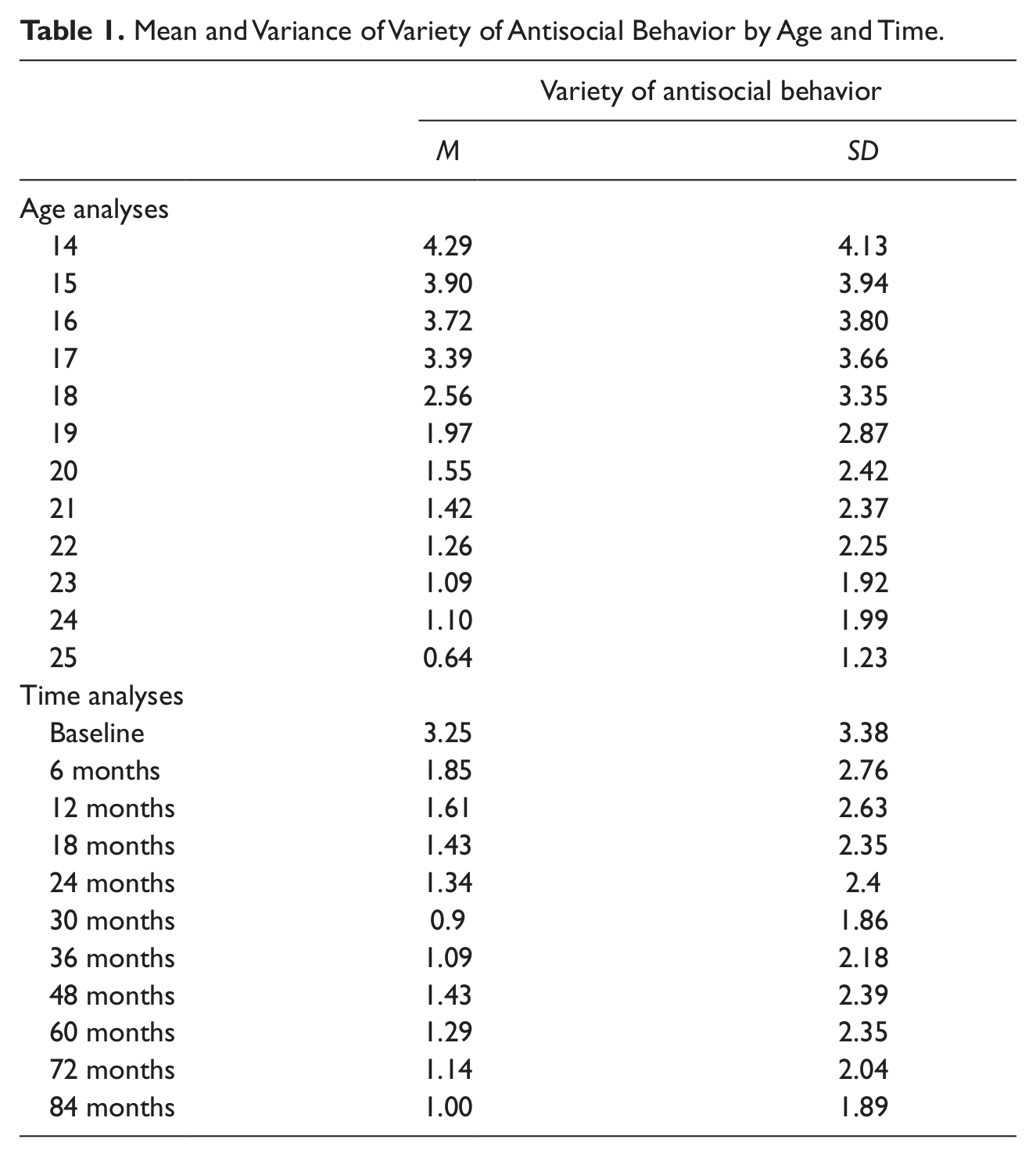
Slightly different measurement approaches were taken with respect to the variety scores based on whether the analyses were conducted by participant’s age or by time of assessment. For models examining antisocial behavior by participant’s age at assessment, time points were combined into annual indicators. This was done so that there was universal measurement across each age (i.e., 14, 15, 16, etc.) and that estimates of antisocial behavior, when distributed by age, were equal (i.e., variety scores at each age reflect a year instead of some reflecting a 6-month recall period and others a yearlong recall period). In contrast, analyses conducted by time do not face this challenge. Consequently, the study design time frame is used (i.e., 3 years with a 6-month recall period, 4 years with a yearlong recall period). Table 1 presents the SRO-variety score distribution (in the aggregate) by age and time.
Mean and Variance of Variety of Antisocial Behavior by Age and Time.
Time Incarcerated
Because incarceration can affect the opportunity to engage in antisocial behavior, all the offending data were adjusted for the amount of time the adolescent spent in the community (i.e., not in a detox/drug-treatment program, psychiatric hospital, residential treatment program, or secure institution), as opposed to being incarcerated or in some other secured facility, as a covariate in the trajectory analyses (Piquero et al., 2001).
Individual Characteristics
Individual characteristics were examined to assess whether they differentially predicted antisocial behavior based on analyses by age-at-assessment and time-of-assessment. All individual characteristics used in the analyses were measured at the baseline interview and have been used in previous Pathways studies (e.g., Loughran et al., 2010; Schubert et al., 2010). The following variables were used: (a) Black, coded 1 for Black participants (M = 0.414, SD = 0.492, else = 0); (b) Prior offending, a count of the total number of court referrals experienced prior to the date of the baseline interview (defined as the number of arrests that were brought to the attention of the court, that is, petitions; M = 3.17, SD = 2.217, range = 0-15); (c) Alcohol problems, obtained from the Composite International Diagnostic Interview (CIDI), a highly structured clinical interview based on the Diagnostic and Statistical Manual of Mental Disorders (4th ed.; American Psychiatric Association, 1994) and International Classification of Diseases–10th Revision (ICD-10) diagnostic criteria (Kessler & Üstün, 2004), coded 1 for diagnosis of alcohol abuse/dependency in the previous year (M = 0.078, SD = 0.268, else = 0); (d) Drug problems, obtained from the CIDI, coded 1 for diagnosis of drug abuse/dependency in the previous year (M = 0.185, SD = 0.388, else = 0); (e) Impulse control, calculated as the average of eight items from the Weinberger Adjustment Inventory designed to measure impulse control (M = 2.961, SD = 0.949, range = 1-5; for example, “I say the first thing that comes into my mind without thinking enough about it,” reverse coded) 5 ; and (f) Parental criminality, which measured whether the participant’s biological mother or biological father had ever been arrested (=1 for either mother or father arrested, M = 0.435, SD = 0.495, else = 0). Additional details about these measures may be found at the study website (www.pathwaysstudy.pitt.edu).
Analytic Plan
The goals of the present study were to (a) examine concordance between SRO-variety score trajectories derived by age-at-assessment and time-of-assessment and (b) test whether common predictors of antisocial behavior are differentially related to age-at-assessment versus time-of-assessment SRO-variety score trajectory solutions. Analyses were conducted in three steps. First, we derived appropriate SRO-variety score trajectory solutions based on age-at-assessment and time-of-assessment. Second, we examined the concordance between the solutions. Third, we tested how covariates were related to group membership for the age-at-assessment SRO-variety score trajectories and the time-of-assessment SRO-variety score trajectories.
Group-based trajectory modeling was used to identify subgroups of individuals who followed similar patterns of behavior over time (Nagin, 2005; Nagin & Land, 1993; Piquero, 2008). Because analyses were based on count data, zero-inflated Poisson modeling was used to account for the clustering at zero. In addition to the SRO-variety score trajectory solutions, an estimate of the proportion of the sample that follows each pair of SRO-variety score trajectories is produced. Furthermore, we also estimate the probability that each individual belongs to each of the groups. This probability is calculated on the basis of data and the maximum likelihood parameter estimates associated with the mixture (posterior probability of group membership) and is used to assign individuals to membership in the group to which they have the highest likelihood of being a member. Analyses tested for up to seven latent SRO-variety score trajectory classes, and the Bayesian information criterion (BIC) was used to compare the fit of different models (Jones, Nagin, & Roeder, 2001).
Because of the nature of group-based trajectory modeling, it was important to identify a priori factors to help determine model selection. Three criteria were used to determine the best latent class solution: the lowest BIC value relative to other models tested, a conceptually clear model, and adequate group membership per trajectory (at least 5% of the sample). The number of classes was decided on, and then the form of the polynomial used to capture the shape of each trajectory was selected, with the highest significant polynomial trend included in analyses. 6 After identifying the SRO-variety score trajectories and then comparing the SRO-variety score trajectory solutions from the two different measurement approaches, we then examined how various individual characteristics related to membership in the trajectory groups across the two solutions using cross-tabulations. Finally, regression models were used to test how individual characteristics were related to group membership derived from the age-at-assessment and time-of-assessment SRO-variety score trajectory solutions.
Results
Trajectory Estimations
We begin by presenting the results of the trajectory analyses for the time-of-assessment (Figure 1) and age-at-assessment (Figure 2) measurements. For the time-of-assessment analyses, a five-group solution provided the best fit and average posterior probabilities of group assignment were very high (>.80). Although we recognize the concerns associated with providing labels to the trajectory solutions, we find doing so useful for interpreting the trajectory solutions. The first trajectory, henceforth referred to as “low,” consists of 25.78% of the sample (average posterior probability = .87). The second trajectory, “mid declining,” includes 30.73% of the sample (average posterior probability = .83). The third trajectory, the “high-declining” trajectory, has 21.22% of the sample (average posterior probability = .88). The fourth trajectory, the “low-stable” group, contains 12.08% of the sample (average posterior probability = .86). The fifth trajectory, the “high-rate” trajectory, includes 10.18% of the sample (average posterior probability = .96).

Time-based trajectory solution of SRO-variety.
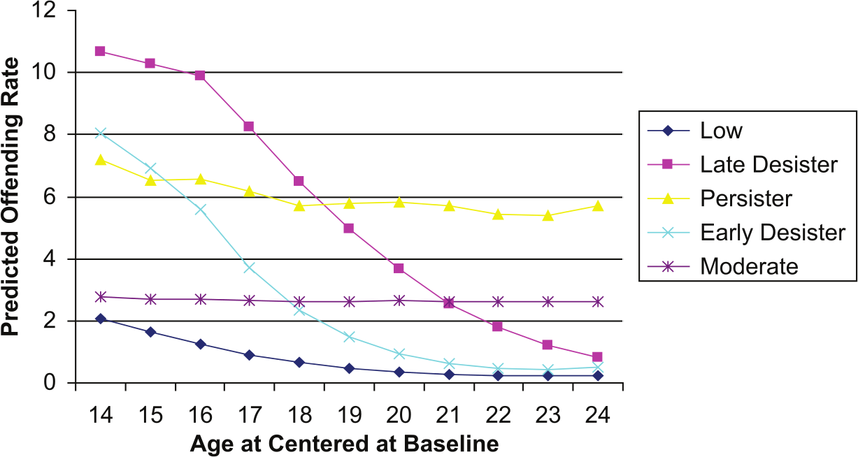
Age-based trajectory solution of SRO-variety.
Four features of this trajectory solution are worth highlighting. First, at the baseline interview, with the exception of the low-stable group, all five trajectories are at their peak SRO-variety score. This is to be expected because the baseline interview covered the period of time immediately prior to the baseline interview, which included the initial juvenile court petition that brought the participant into the study. The drop off between the baseline and initial follow-up (6-month) interview is to be expected, in part, because of a sizable incarceration effect that removed many juveniles from the community. Second, high-rate offenders have higher rates of SRO-variety throughout the entire observation period and evince a small decrease beginning around the 48th month through the 84th month of follow-up. Third, the high-declining and high-rate trajectories exhibit similar SRO-variety scores at the outset, but soon thereafter, individuals in these groups begin to display two distinct trajectories of offending, with the high-declining group decreasing to very little offending, whereas the high-rate group remaining high with a score of almost 4.0 at the 84-month interview. Finally, two of the trajectory groups (low and mid declining) have similar trends from baseline through the 84-month interview, with the mid-declining group showing a slightly higher SRO-variety score.
Similar to the time-at-assessment, the age-at-assessment trajectory analysis demonstrated that a five-group solution provided the best fit (see Figure 2). The first group, “low,” consisted of individuals who reported low levels of offending at every age (37.22% of the sample, average posterior probability = .90). The second group, the “late-desister” group (10.48% of the sample, average posterior probability = .85) exhibited the highest SRO-variety at baseline through about age 18 and then declined in SRO-variety as they transitioned to adulthood. The third group, “persisters,” reported a consistently high variety of antisocial behavior from adolescence into early adulthood (7.54% of the sample, average posterior probability = .85). The fourth group, “early desisters” (31.25% of the sample, average posterior probability = .85), resembled the late desisters but showed lower levels of antisocial behavior in early adolescence and quickly desisted from crime as they entered early adulthood. Finally, the “moderate” group (13.51% of the sample, average posterior probability = .81) consisted of individuals who exhibited moderate but constant levels of SRO-variety between adolescence and early adulthood.
Also seen in Figure 2, there are sizable differences in SRO-variety levels across the groups, with late desisters starting off at the highest point but then dropping noticeably in late adolescence and into early adulthood. Two groups, persisters and moderates, had stable offending patterns over the age range, with individuals in the persister trajectory still averaging around six different offense types in the mid-20s—virtually the same level they were at in the mid-teens. Last, the persisters and early desisters start at virtually the same level of SRO-variety (with early desisters actually showing a higher starting point) but end up at very different places by their mid-20s, with persisters still averaging almost six different offenses, whereas early desisters averaging almost none.
There are some distinctions in the trajectory solutions shown in Figures 1 and 2 that are noteworthy. More generally, the two sets of solutions have different shapes overall and they peak at different points as well. A more specific difference can be seen in that more than 20% of the sample in the age-based solution follows a stable (moderate and persister) trajectory, whereas none of the trajectories in the time-based solution are stable, and in fact, one of the trajectories (low stable) is increasing. The two solutions appear to generate trajectories that are distinct in function and form.
Concordance Between Trajectories Based on Different Measurement Approaches
Next, we consider how the two solutions relate to one another. 7 As seen in Table 2, there is a modest but not perfect concordance across the two different solutions, with higher concordance found at the extremes (i.e., very low or very high antisocial behavior relative to other trajectory groups). For ease of presentation, we present these results through the lens of each trajectory solution.
Relation Between Time-Based Trajectory Solution and Age-Based Trajectory Solution.

From the perspective of the time-of-assessment solution, of the 271 individuals in the low group, 86.35% (n = 234) are distributed in the low group from the age-at-assessment trajectory solution. Among the 323 members of the mid-declining group, there is an approximately even split across two groups from the age-based solution, with 48% in the low (n = 154) and 45% (n = 144) in the early-desister trajectories. Given the SRO-variety rates across all three of these trajectories, these results seem to capture substantively similar rates/trends of offending. There is somewhat more ambiguity when looking at the distribution of the high-declining group from the time-based solution and how these individuals are distributed across the age-based solution. In particular, of the 223 individuals in the high-declining time-based trajectory group, 23% are in the late-desister age-based trajectory group (n = 52), 10% are in the moderate (n = 22) group, and almost two thirds (62.33%, n = 139) are in the early-desister group. Among the 127 individuals in the low-stable time-based trajectory group, 76.38% (n = 97) are found among the moderate age-based trajectory group, with the rest distributed across three of the other four groups (with only one person in the low age-based solution). Last, among the 107 individuals in the high-rate time-based trajectory group, 41% were classified as late desister (n = 44) and 57% were classified as persisters (n = 61) in the age-based trajectory groups.
Examining the cross-tabulation from the age-based trajectory perspective, of the 392 individuals in the low group, 60% (n = 234) were classified as being in the low time-based trajectory group and 39% (n = 154) were classified as being in the mid-declining time-based trajectory group. Of the 108 age-based late-desister group, 48% (n = 52) were classified as high declining and 41% (n = 44) were classified as high rate in the time-based trajectories. The 80 persisters from the age-based trajectory were grouped primarily in the high-rate trajectory (76%, n = 61), whereas 68% (n = 97) of the 143 individuals in the age-based moderate offender group are found in the low-stable group from the time-based solution. The largest discrepancy concerned the 328 age-based early-desister individuals, who were spread in two main groups from the time-based solution, the mid-declining (44%, n = 144) and high-declining (42%, n = 139) groups. Finally, among the 143 persons in the age-based moderate group, about 68% (n = 97) were in the time-based low-stable group. 8
Relationship Between Risk/Protective Factors and Trajectory Groups
The final portion of our investigation examines how several individual characteristics distinguish between the trajectory group memberships that emerged from each of the two measurement approaches. Tables 3 and 4 present these results in a bivariate fashion for the time-based and age-based approaches, respectively, whereas Tables 5 and 6 consider the risk/protective factors jointly in a multivariate manner.
Bivariate Relation Between Risk/Protective Variables and Trajectory Group Membership Using Time-of-Assessment Measurement, M (SD).

p < .05.
Bivariate Relationship Between Risk/Protective Variables and Trajectory Group Membership Using Age-at-Assessment Measurement, M (SD).
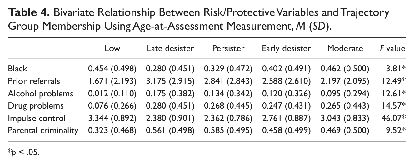
p < .05.
Multinomial Logistic Regression Predicting Survey—Time-Based Trajectories.
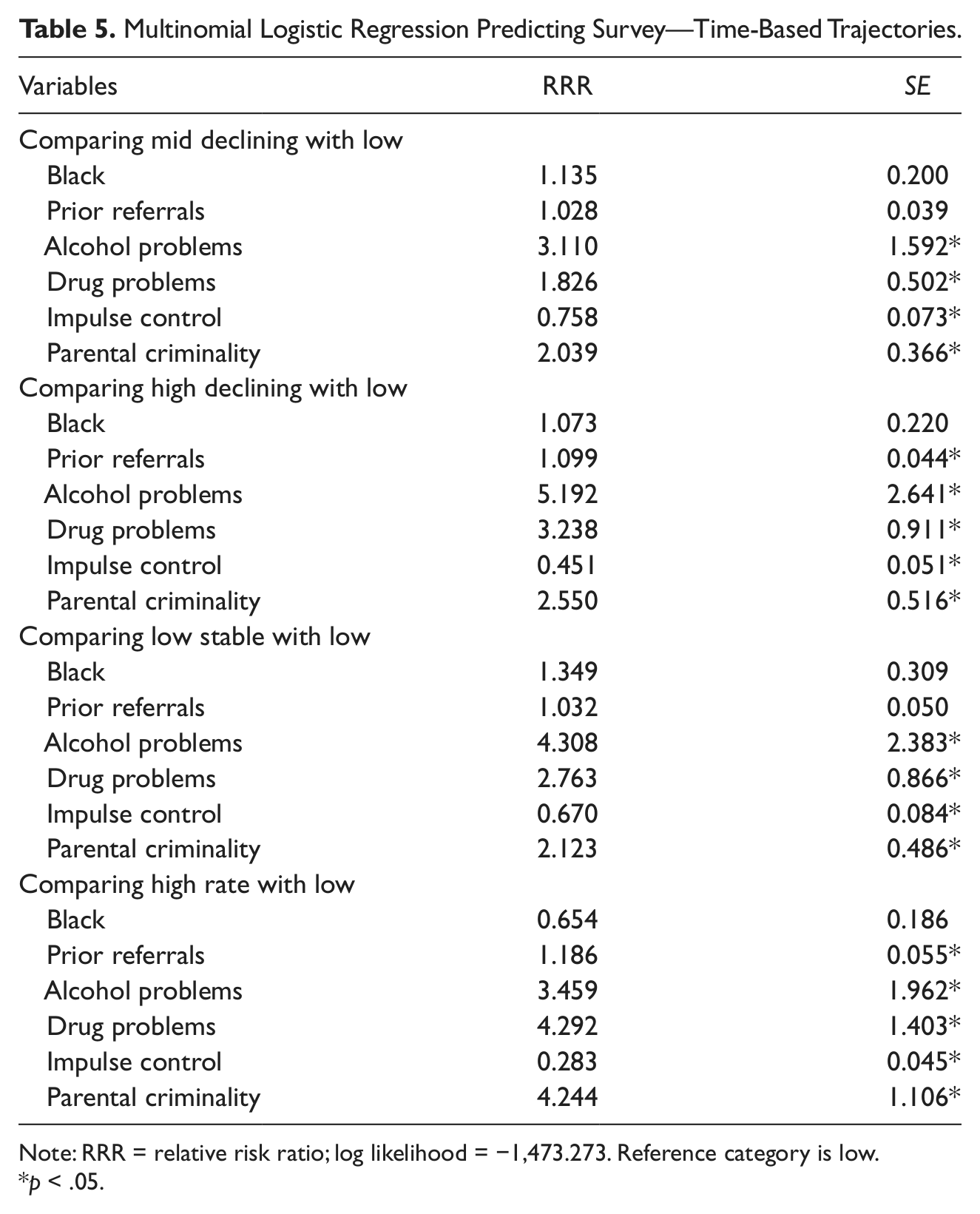
Note: RRR = relative risk ratio; log likelihood = −1,473.273. Reference category is low.
p < .05.
Multinomial Logistic Regression Predicting Age-Based Trajectories.

Note: RRR = relative risk ratio; log likelihood = −1,403.594. Reference category is low.
p < .05.
As can be seen from the time-based trajectories shown in Table 3, prior referrals are highest among the high-rate group (M = 3.373) and lowest among the low group (M = 1.789), whereas the high-rate group displays the lowest impulse control (M = 2.265) and the low group displays the highest impulse control (M = 3.323). Turning to the age-based results in Table 4, it can be seen that impulse control is lowest among the persisters (M = 2.362) but highest among the low group (M = 3.344), whereas parental criminality is highest among persisters (M = 0.585) but lowest in the low group (M = 0.323). All the comparisons are significant in Tables 3 and 4 across the groups with the low group always having less risk and higher impulse control, whereas the opposite is true for the most chronic of offenders—regardless of measurement approach.
Next, we examine the risk/protective variables in a multivariate framework for distinguishing between trajectory group memberships. Table 5 presents the results from the time-based trajectories, whereas Table 6 displays the results from the age-based trajectories. For the multinomial logistic regression models presented, the low trajectory is the reference category, primarily because the highest overlap across measurement approaches was found in this least-extreme offending group.
With respect to the time-based trajectory analyses, it can be seen that compared with the low trajectory, most of the variables have their anticipated association with the specific offending trajectory. For example, low-stable offenders are distinguished from low offenders by having more alcohol and drug problems as well as being more likely to have parents with a prior criminal history. Impulse control is lower among low-stable offenders compared with low offenders. Comparing low offenders with high-declining offenders reveals a similar set of results with the addition that number of prior referrals is significantly associated with the high-declining trajectory. Comparing low trajectories with mid-declining trajectories indicates again that alcohol and drug problems as well as parental criminality are associated with membership in the mid-declining group, whereas impulse control is associated with membership in the low group. Finally, high-rate offenders are more likely than low offenders to have more prior referrals, alcohol and drug problems, and parents who have a prior criminal history, whereas low offenders have higher impulse control. Across all comparisons, being Black did not distinguish between trajectories.
In the age-based trajectories, the pattern of findings distinguishing the low trajectory from the other offender trajectories is remarkably consistent across all the comparisons. Specifically, all the offenders in the non-low trajectory average a greater number of prior referrals, more alcohol and drug problems, more parents with a prior criminal history, and poorer impulse control. Being Black did not differentiate being in any of the specific age-based trajectory groups. Overall, the multinomial logistic regression analyses showed a highly consistent pattern of covariate associations across the time- and age-based solutions, but it is worth noting that the coefficients in the age- and time-based solutions do vary in magnitude.
Discussion
Based on their specific empirical question of interest, researchers have the option to model longitudinal data by age or by time, and these options provide valuable information, depending on the question of interest. Given that there are multiple data sets available to those interested in longitudinal offending patterns (i.e., NYS and the Adolescent Health Survey), it is important to understand how modeling decisions alter substantive conclusions. In the current study, we use the same data to assess whether the modeling decision (age vs. time) leads to substantively different conclusions about longitudinal offending patterns generally and predictors of offending in particular. Two key findings emerged from our investigation of these issues.
First, there was a general consensus between the two solutions, particularly at the low and high ends of the offending distribution. For example, both approaches identified a similar number of individuals who were engaged in very low rates of offending and similarly identified a group of individuals engaged in high or very high rates of offending. Thus, at the extremes of the offending distribution, the time-based and age-based approaches tend to identify similar sets of individuals. At the same time, there was more ambiguity regarding mid-range offenders, as the concordance of the methods in identifying similar offenders who evince similar offending patterns was not consistently high (but the average scores on the covariates assessed did not vary demonstrably across the midrange groups). Furthermore, in addition to evincing different overall shapes and peaking at different points, the age-based solution provides evidence of a stable set of trajectories (moderate and persister) that is not perfectly replicated in the time-based solution.
Second, an examination of how several correlates distinguished between trajectory groups in each of the two estimation procedures pointed to a substantively similar set of results as all the variables distinguished between the low offender trajectory and their more chronic offender trajectory counterparts as expected. Moreover, substantively similar conclusions were reached with respect to the average values of risk/protective factors across the trajectory groups in the two measurement solutions, especially between the two extreme offender groups: The lowest-risk group always displayed the least risk but most impulse control, whereas the most chronic group displayed the most risk and least impulse control. Still, it is notable that the coefficients in the age- and time-based solutions did vary in magnitude.
In short, regardless of the x-axis decision (time or age), there is less ambiguity in trajectory group size, shape, and membership in the extremes of the trajectory solutions (least and most chronic offenders), but there is more variability in between the extreme groups. In addition, in the time-based and age-based solutions, several risk/protective factors distinguished between groups in substantively similar ways, but when considered multivariately, several of the coefficients varied in magnitude across the time- and age-based solutions. It may be that much of the similarity is due to the nature of the specific sample being studied. The Pathways sample contains a group of serious adolescent offenders, who were age 16, on average, at the initial study assessment. Thus, the rather constricted nature of the ages at the time of the initial survey may have produced a sample that was more alike than different with respect to their placement on the offending continuum. This constricted age range is not the norm in most general population, publicly available longitudinal studies, such as the NYS, NLSY, or Add Health, which contain a much broader range of ages in the initial interview. It could be that the larger spread of ages and background characteristics in those data sources, especially in the NYS, to include prepubescent youth compared with late teenage youth who are at very different points in the age/crime continuum (Lauritsen, 1998) may make the measurement issue more pronounced. It could also be that because the present sample consists of persons who are all known offenders, we may have captured a different distribution of antisocial acts. Notably, however, the solutions derived in this sample mirror trajectories derived from community-based samples (see Piquero, 2008).
Going forward, there is a need to further consider and address potential problems related to separating the effects of repeated testing from potential developmental processes (Lauritsen, 1998). One way to minimize problems associated with studying SRO and the problems it creates is to include external measures of a person’s antisocial behavior (official arrest records, parent and/or peer reports, etc.). This, along with replication of our analyses with other nonoffender data sources, will provide important evidence regarding the extent to which the unit of measurement is another methodological challenge facing longitudinal studies of criminal activity. Until then, it is noteworthy that whether a researcher focuses analyses based on time or age should be driven by the research questions at hand. Inquiries aimed at generating policy relevant information about how samples of serious offenders respond to particular life changes or involvement in services would likely be more interested in differential effects related to time-based trajectory group membership. However, for analyses that are focused on how behavior changes with age-related developmental changes (as is usually the case with antisocial and criminal behavior), then it makes sense to consider the more relevant age-related trajectories. It appears that, although there seems to be no more consistent correlate of crime than age, the factors related to altered patterns of offending are similar whether modeled as age based or time based.
Footnotes
Appendix A
Authors’ Note
The content of this article, however, is solely the responsibility of the authors and does not necessarily represent the official views of these agencies.
Declaration of Conflicting Interests
The author(s) declared no potential conflicts of interest with respect to the research, authorship, and/or publication of this article.
Funding
The author(s) disclosed receipt of the following financial support for the research, authorship, and/or publication of this article: Office of Juvenile Justice and Delinquency Prevention (2007-MU-FX-0002), National Institute of Justice (2008-IJ-CX-0023), John D. and Catherine T. MacArthur Foundation, William T. Grant Foundation, Robert Wood Johnson Foundation, William Penn Foundation, Center for Disease Control, National Institute on Drug Abuse (R01DA019697), Pennsylvania Commission on Crime and Delinquency, and the Arizona Governor’s Justice Commission.