



Abstract
Unit non-response is a serious problem in survey research. This article validates the necessity of adjusting for unit non-response in disproportionate stratified sampling designs through the use of sample weights. Using data from the 1958 Birth Cohort study, we demonstrate that sample data which are affected by unit non-response can be a poor representation of population parameters. These non-response effects can be addressed through the application of sample weights.
Introduction
The purpose of this article is to complement a previous article (Tracy & Carkin, 2014), which demonstrated that inferential and statistical modeling problems can arise if researchers fail to appreciate the implications of sampling design and, especially, when disproportionate stratified sampling is used. The previous article validated the necessity of adjusting for the design effects in disproportionate stratified sampling designs through the use of sample weights. Using data from the 1958 Birth Cohort study, we demonstrated that complex sampling designs introduce sampling error, and even sampling bias, into sample data. Consequently, unweighted data from complex sampling designs are a poor representation of population parameters. We provided empirical results which showed that these design effects must be remedied through the use of sample weights. This article extends the issue by showing that sample data must also be weighted to deal with unit non-response.
Data and Method
We again draw upon the data from the 1958 Birth Cohort study (Tracy, Wolfgang, & Figlio, 1990). Because we have provided extensive details about the sample methodology used in that study elsewhere (Tracy & Carkin, 2014), we only briefly summarize here the design. The 1958 Birth Cohort Follow-Up used a sampling design which guaranteed that cases would be sampled across important characteristics of the cohort—a stratified random sampling scheme which yielded 26 sample strata produced from the combinations of sex, race/ethnicity, socio-economic status (SES), number of juvenile offenses, and number of juvenile status offenses. To ensure that high-risk cases were available in the sample in sufficient numbers to permit meaningful analyses, a disproportionate sample selection method was used.
Sampling Error/Non-Response Bias
Sample Attrition: Surveyed Versus Not Surveyed
Anyone familiar with field-based survey research knows that social surveys must confront the problem of non-response. In spite of best efforts for collecting data from a sample, non-response nearly always occurs in survey research. Such non-response appears to be increasing. de Leeuw and de Heer (2002) have indicated that in recent decades, developed countries have seen an increase in the rate of sample persons not being measured. Similarly, in a comprehensive analysis of the state of survey research, Groves (2006) has shown that as non-response rates increase in household surveys, non-response bias studies become increasingly important (indeed, they are called for by recent Office of Management and Budget Guidelines, 2006 for U.S. federal government–funded surveys.
A “non-respondent” is any unit or case that is eligible for a study but for which data are not obtained for any reason. Some sample members cannot be located, whereas others refuse to be interviewed. These non-sampling errors as they are called are quite prevalent in survey research. The question arises, therefore, concerning the extent to which sample attrition is associated or correlated with respondent characteristics. If such attrition is differentially distributed across respondent categories, in this case the matrix of 26 sample strata, then a situation of non-response bias could be said to exist.
The results concerning the tracking success of the drawn sample are reported in Table 1. The search for the drawn sample of 1,992 cases (1,524 males and 468 females) resulted in a total of 783 completed surveys. Table 1 presents a layout concerning whether a drawn sample member was surveyed versus not surveyed across the six sample strata for females. Completed surveys were obtained for 202, or 43% of the drawn sample. The results by individual stratum show that the lowest percentage was 33% for non-White non-offenders, whereas the highest percentage was obtained for White recidivists with two or more offenses (58%). Taken together, we note that the data show a 47.8% completion rate for White females (112 out of a possible 234) and a 38.5% completion rate for non-White females (90 out of a possible 234). Although slightly different, the completion rates across the female strata do not produce any significant differences for attrition by race. For the 20 strata of our male sample, overall, we have completed interviews with 581 males for a completion rate of 38%.
Drawn Sample Response/Non-Response Results.
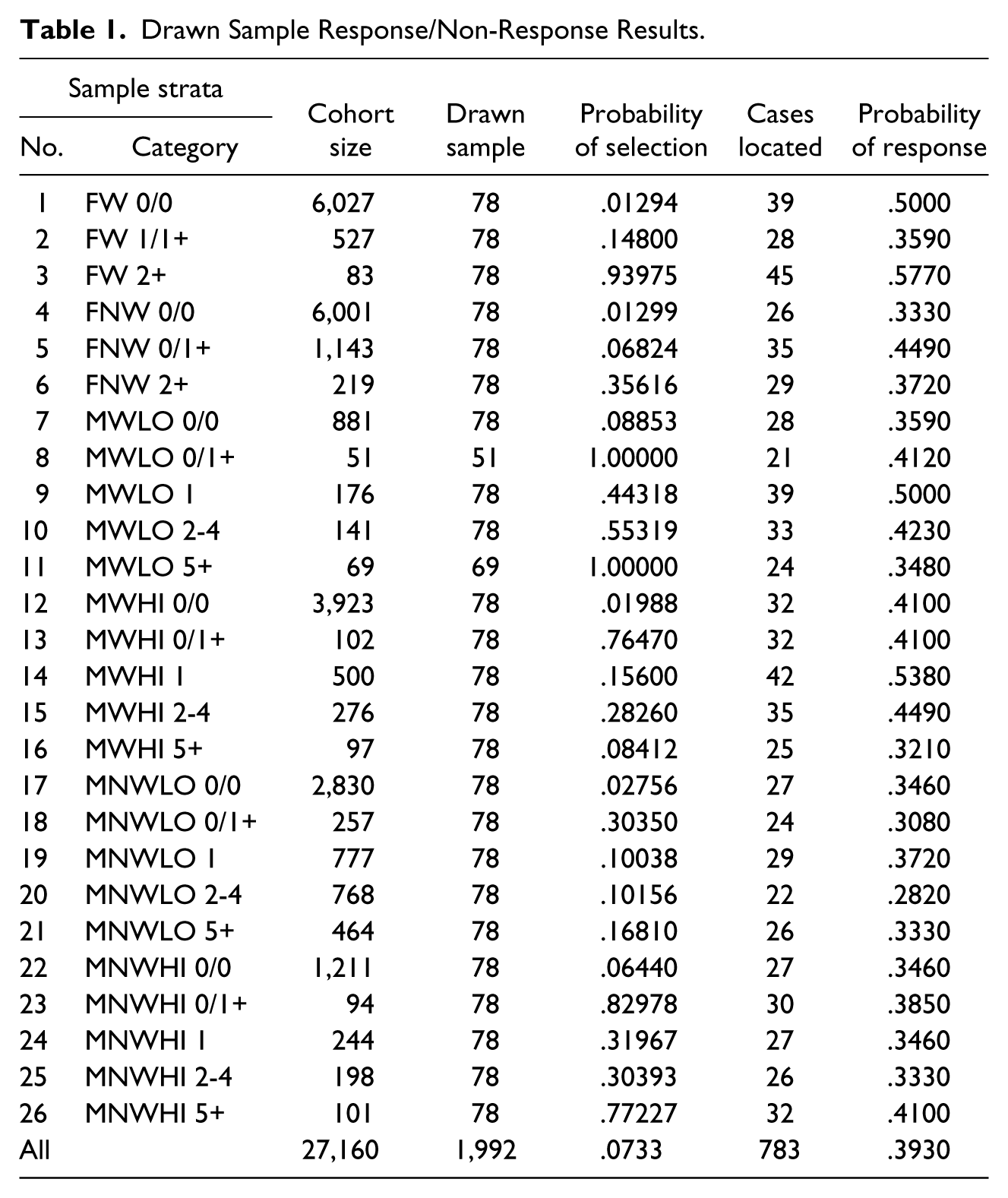
When we examine this completion percentage across the 20 male sample strata, we observe the following. First, the highest completion percentage is 54% for the White, high SES, one-time offender, whereas the lowest completion rate was obtained for the non-White, low SES, non-chronic offender (two to four offenses) with 28% completed surveys. Furthermore, we note that was the only male stratum with a completion rate in the 20% range; 11 strata were in the 30% range, 6 strata were in the 40% range, and 2 were in the 50% range.
Fortunately, chi-square tests indicate that there were no significant difference between cases surveyed and those not surveyed across any sample strata. Another way to test whether there are any cohort characteristics that are associated with the status of survey response versus non-response is to perform a logistic regression analysis with background characteristics regressed on a dummy dependent variable which captures survey versus non-survey status. The results of such a model are shown in Table 2. The logistic model used the following variables: (a) main effects: Male, White, SES, One-time delinquent, 2 to 4 times recidivist, and chronic recidivist and (b) interaction effects: SES × White, SES × Sex, and Sex × White. There were no coefficients that were significantly related to survey status. We may conclude, therefore, that there are no systematic biases surrounding which sample cases were interviewed and which were not. However, it remains to be determined whether the scores on important criterion measures show bias, that is, a difference between the scores of respondents versus non-respondents (Kalsbeek, Morris, & Vaughn, 2001).
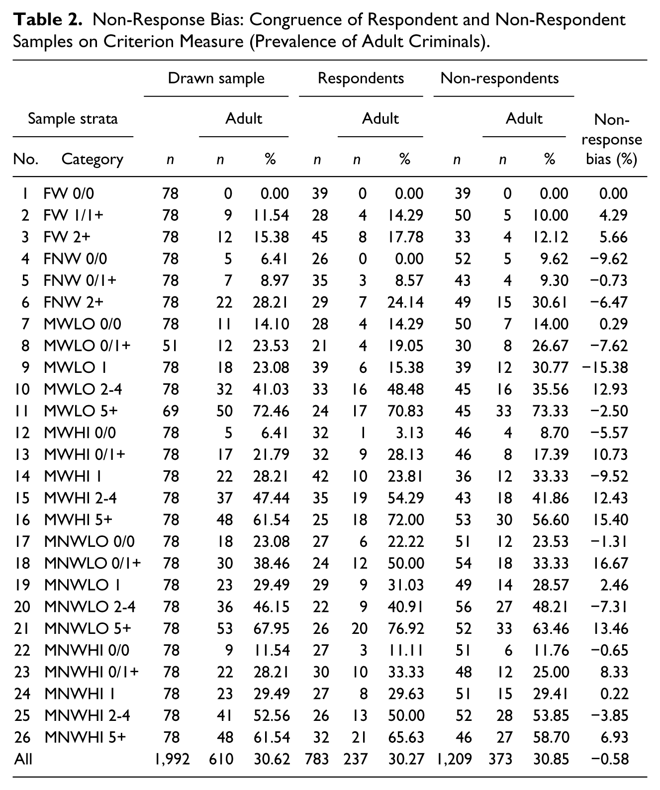
Non-Response Bias: Congruence of Respondent and Non-Respondent Samples on Criterion Measure (Prevalence of Adult Criminals).
Sample Attrition: Surveyed Versus Not Surveyed—Criterion Measures
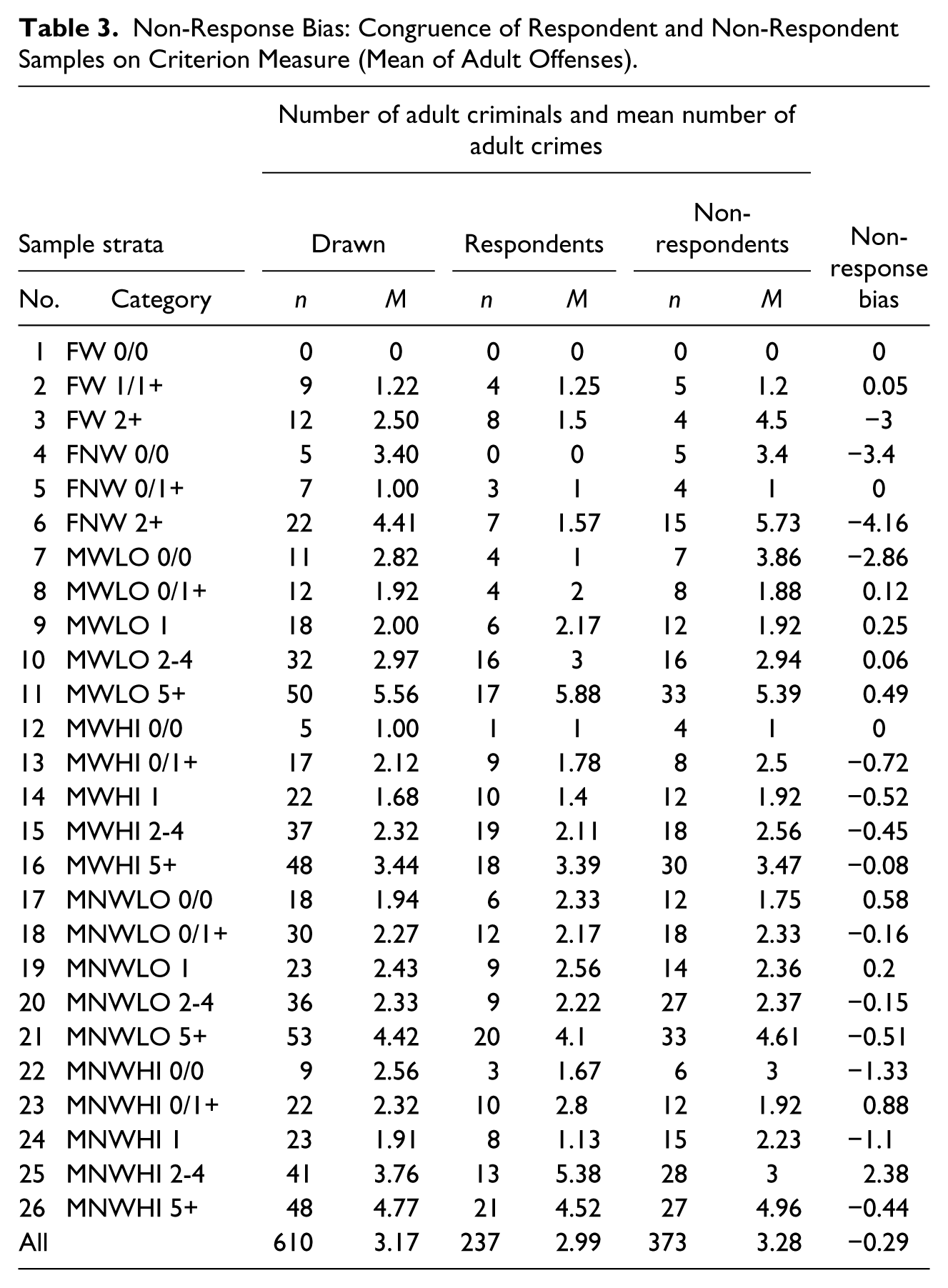
We now examine the congruence between the drawn sample sub-groups (interviewed vs. non-interviewed) to see if there are significant differences with respect to the same two criterion measures that we used in the previous article: (a) adult prevalence and (b) adult incidence. Table 3 indicates that, overall, the interview group (30.27%) and the not interviewed group (30.85%) only differ by 0.58 percentage points in terms of adult offender status. Yet, Table 3 also shows that across the various strata there are notable differences. For some strata, like male/non-White/low SES/one or more status offenses, respondents contain up to about 16.67% more adult criminals, whereas for other strata, like male/White/low/one or more delinquencies, the non-response group contains up to 15.38% more adult criminals. Generally, however, the differences are less pronounced and the disparities cancel one another out, thus yielding a very close overall percentage. The results displayed in Table 4 for the mean number of adult crimes reflect even stronger that the two sub-samples are not significantly disparate. Overall, the respondent sub-sample committed 2.99 adult crimes, whereas the non-respondent sub-sample committed 3.28, a difference of just 0.29 adult crimes per offender. The differences across the various strata are not very appreciable except for a few strata for which a very small number of adult criminals affected the mean score comparisons.
Non-Response Bias: Congruence of Respondent and Non-Respondent Samples on Criterion Measure (Mean of Adult Offenses).
Estimation Bias: Congruence of Drawn and Response Samples on Criterion Measure (Prevalence of Adult Criminals).
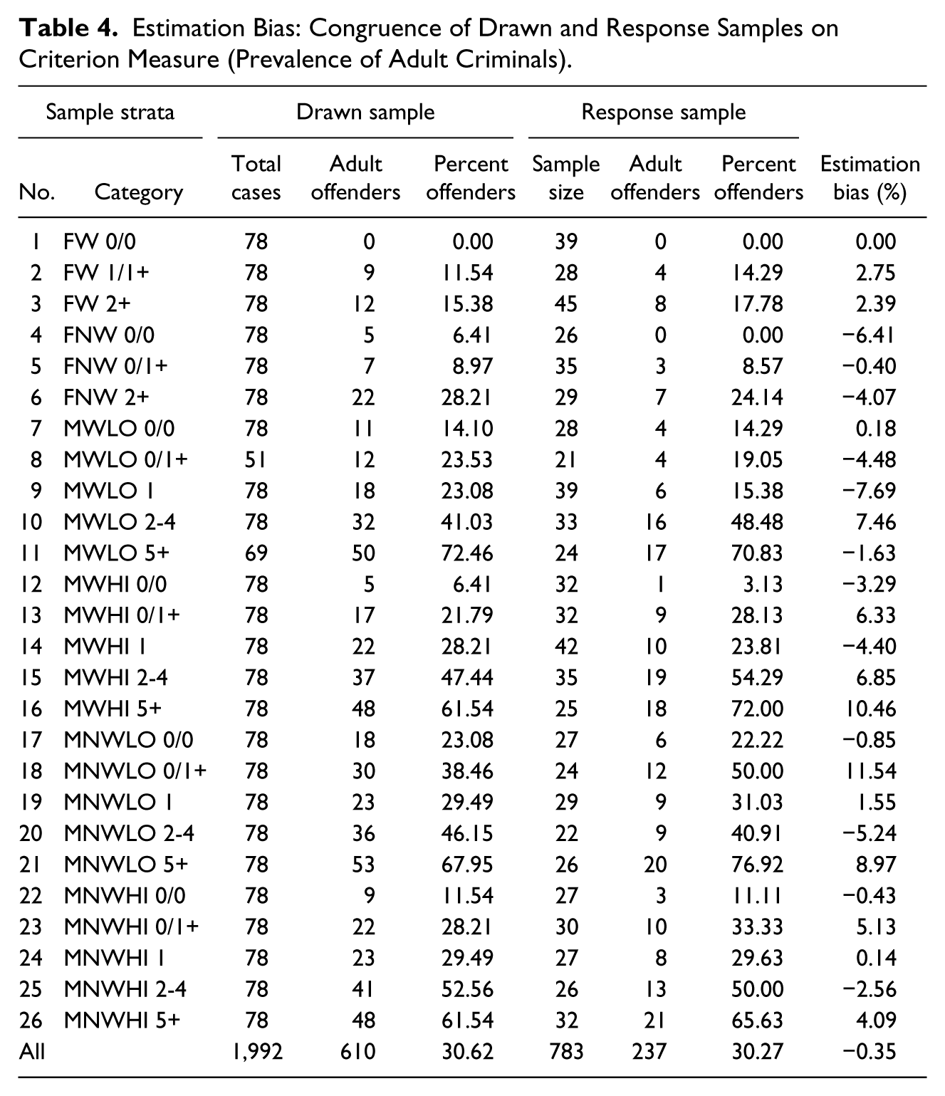
Tables 3 and 4 thus indicate that the sub-sample that was interviewed, as compared with the sub-sample that was not, does not show any consistent pattern to suggest that the interviewed group was systematically and significantly biased either upward or downward in terms of the percentage of adult criminals or the extent of their criminal offenses. Having established this, we can now examine whether using the interviewed sample to generate estimates of population data (the full cohort) is statistically reasonable or whether we risk the likelihood of estimation biases. These results are displayed in Tables 5 and 6.
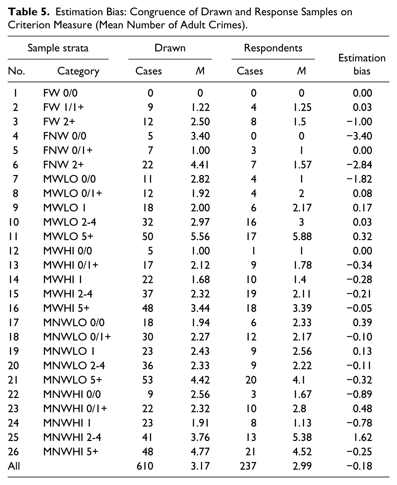
Estimation Bias: Congruence of Drawn and Response Samples on Criterion Measure (Mean Number of Adult Crimes).
Interview Sample Response Weights.
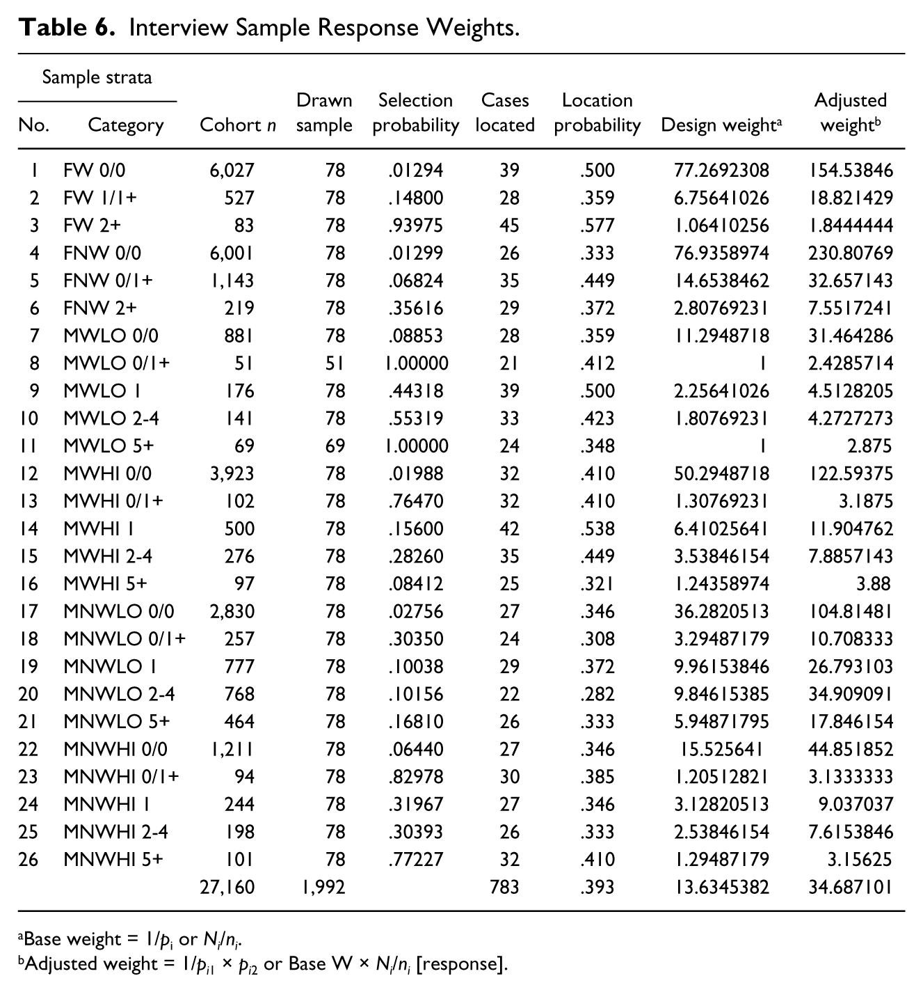
Base weight = 1/pi or Ni/ni.
Adjusted weight = 1/pi1 × pi2 or Base W × Ni/ni [response].
Table 5 indicates that, overall, the interviewed sample contains 30.27% adult offenders as compared with the drawn sample which had 30.62% (an underestimate of just 0.35%). Across the various strata, the largest differential occurs for male/non-White/low SES/one or more status offenses (+11.54%), the male/White/high SES/chronic delinquents (+10.46%), and the male/non-White/low SES/chronic delinquents (+8.97%). Beyond these three highest differences between the interviewed and drawn samples, the rest of the strata show only modest or no appreciable differences. Table 6 confirms with respect to the mean number of adult crimes committed by the interview sample (2.99) is nearly the same as that for the drawn sample (3.17). Moreover, there were very few individual strata for which the difference in means was especially problematic except for female non-Whites with no delinquencies or status offenses. For this group, the drawn sample had a frequency of 5 with a mean of 3.40, whereas the interviewed sample had no such cases thus causing the difference.
Interview Sample: Two-Stage Weighting
When non-response occurs, the researcher must implement a weight adjustment process to compensate for the loss of the non-response cases because the interviewed sub-sample no longer represents the drawn sample, and in turn, the interview sub-sample surely does not represent the population. This non-response weight adjustment process increases the weights of the sampled cases for which data were collected (Little & Vartivarian, 2003; Rao, Sigurdson, Doody, & Graubard, 2005). This is a second-stage procedure to the Base Weight adjustments for the differential selection probabilities across sample strata (Tracy & Carkin, 2014). In a disproportionate stratified sampling situation, this represents a second-stage weighting process that is now necessary to accommodate the fact that interviewed respondents across strata have a second-order selection probability at work. That is, there were differential probabilities of being selected for the sample in the first place, and now there is a second probability at work (i.e., the probability of being interviewed), and these two probabilities differ across the various strata (Mohadjer & Choudhry, 2002). This second-stage weighting scheme produces what are called adjusted weights, which are calculated as follows:

where p1 = probability of selection and p2 = probability of interview.

where N = cases in drawn sample strata and ni = interviewed cases in strata.

where N = cases in drawn sample strata and ni = interviewed cases in strata.
These formulae are equivalent and can all be derived algebraically from one another. It would seem that Equation 1 is the easiest to conceptualize and implement. Equation 1 draws upon the multiplication rule from probability theory—the probability of a joint event which consists of two separate independent events is Probability 1 × Probability 2. For example, if we toss a fair coin twice, the probability that we will obtain two (Equation 2) heads is 0.5 × 0.5 = 0.25, or a 1/4 chance. Inspection of the possible outcomes proves this: (a) head–head, (b) head–tail, (c) tail–head, and (d) tail–tail.
The adjusted weights for the 1958 Birth Cohort study are reported in Table 7. These adjusted weights result in the counting of each case in the interview sample strata a certain number of times to represent the cohort members in a given strata. Cases are counted from a high of 154 times for White females with no delinquencies or status offenses to a low of 1.8 times for White females with two or more offenses. The fundamental objective of the design of any survey sample is to produce a survey data set, that, for a given cost of data collection, will produce statistics that are nearly unbiased and sufficiently precise to satisfy the goals of the expected analyses of the data. In general, the goal is to keep the mean square error (MSE) of the primary statistics of interest as low as possible. MSE is a very important measure and is calculated as follows:

where Bias = (: − 0).
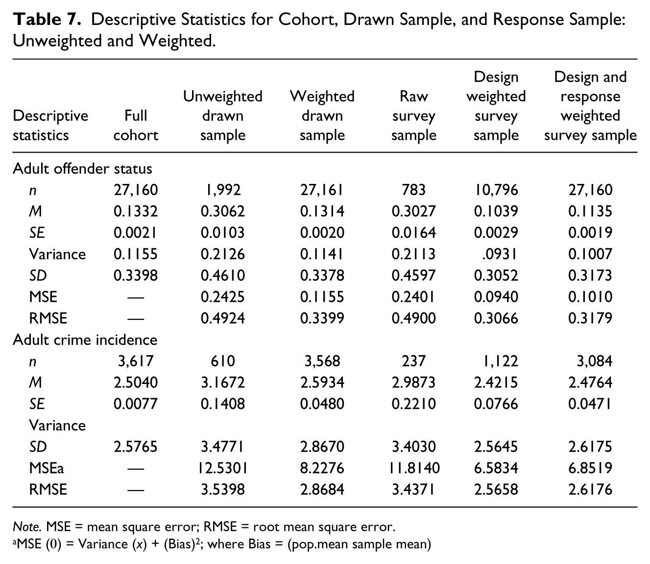
Descriptive Statistics for Cohort, Drawn Sample, and Response Sample: Unweighted and Weighted.
Note. MSE = mean square error; RMSE = root mean square error.
MSE (0) = Variance (x) + (Bias)2; where Bias = (pop.mean sample mean)
Essentially, the MSE of any sample statistic inflates the variance of the estimate by the bias surrounding the sample statistic. Here, bias is the difference between the cohort mean (:) and the sample mean (0). Thus, as the sample mean departs from the population mean, MSE becomes increasingly greater than the variance. Likewise, because root mean square error (RMSE) is analogous to the standard deviation, as the sample standard deviation departs from the population standard deviation, RMSE becomes increasingly greater than the standard deviation.
The purpose of the weighting adjustments shown in Table 7 is to reduce the bias associated with non-response in the survey. Thus, the application of weighting adjustments usually results in lower bias in the associated survey statistics, but at the same time, adjustments may result in some increases in variances of the survey estimates. The increases in variance result from the added variability in the sampling weights due to non-response. Thus, when analysts create the weighting adjustment, they need to pay careful attention to the variability in the sampling weights caused by these adjustments. The variability in weights will reduce the precision of the estimates. Thus, a trade-off should be made between variance and bias to keep the MSE as low as possible. However, there is no exact rule for this trade-off because the amount of bias is unknown.
In general, weighting adjustments frequently result in increases in the variance of survey estimates when many weighting classes are created with a few respondents in each class, and some weighting classes have very large adjustment factors (possibly due to much higher non-response or low initial selection probabilities in these strata). Occasionally, the procedures used to create the weights may result in a few cases with extremely large weights. Extreme weights can seriously inflate the variance of survey estimates. “Weight trimming” procedures might need to be used to reduce the impact of such large weights on the estimates produced from the sample. Weight trimming refers to the process of adjusting a few extreme weights to reduce their impact on the weighted estimates (i.e., increase in the variances of the estimates). Trimming introduces a bias in the estimates; however, most statisticians believe that the resulting reduction in variance decreases the MSE. Thus, analysts should pay attention to the variability of the weights when working with survey data, even though all measures (such as limits on adjustment cell sizes, and weight trimming) may have been taken to keep the variability of weights in moderation. Analysts should keep in mind that large variable values in conjunction with large weights may result in extremely influential observations, that is, observations that dominate the analysis.
Table 7 provides descriptive statistics for the two criterion measures we have been examining: proportion of adult criminals (prevalence) and mean number of adult crimes (incidence). We saw before with respect to prevalence, that the unweighted drawn sample is a poor representation of the full cohort. The mean, variance, standard deviation, and standard error are all much higher in the unweighted drawn sample. After weighting, the sample data now are virtually identical to the full cohort scores for all the usual descriptive statistics (mean, variance, standard deviation, and standard error). Table 8 adds three more columns to the data to show the descriptive data for the raw interview sample, the interviewed sample after applying design weights (Stage 1), and finally the interviewed sample with adjusted weights (Stages 1 and 2). How well does the adjusted interview sample represent the full cohort? Nearly perfectly!
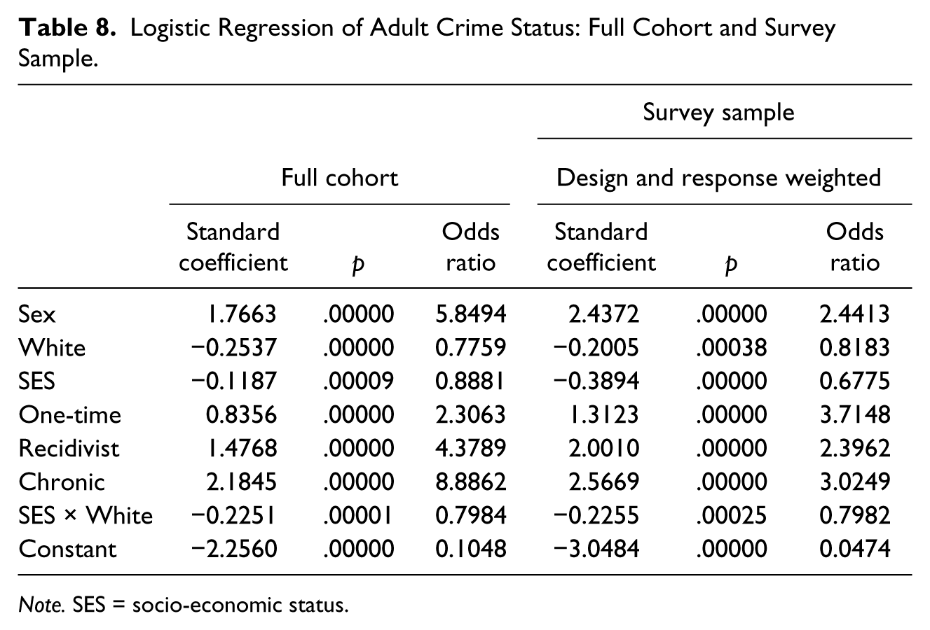
Logistic Regression of Adult Crime Status: Full Cohort and Survey Sample.
Note. SES = socio-economic status.
Concerning the prevalence of adult criminals: The means are very close (0.1135 vs. 0.1332); the standard errors are close and favor the sample (0.0019 vs. 0.0021), and the variance is lower in the sample (0.1007 vs. 0.1155). The MSE statistics confirm that we have not introduced bias, even though some of the adjusted weights were quite large. That is, the MSE of the sample (0.1010) is virtually identical to the variance in the sample (0.1007) and they are both lower than the variance in the cohort (0.1155).
We also did exceedingly well with respect to the other criterion measure—the incidence of adult crimes. The mean in the adjusted sample only slightly underestimates the mean of the cohort (2.48 vs. 2.50); the standard errors are close (0.0471 vs. 0.0077), and the variance is only slightly higher in the sample (6.8513 vs. 6.6384). As above, the MSE statistics confirm that we have not introduced bias, even though some of the adjusted weights were quite large. That is, the MSE of the sample (6.8519) is virtually identical to the variance in the sample (6.8513) and they are both are practically the same as the variance in the cohort (6.6384).
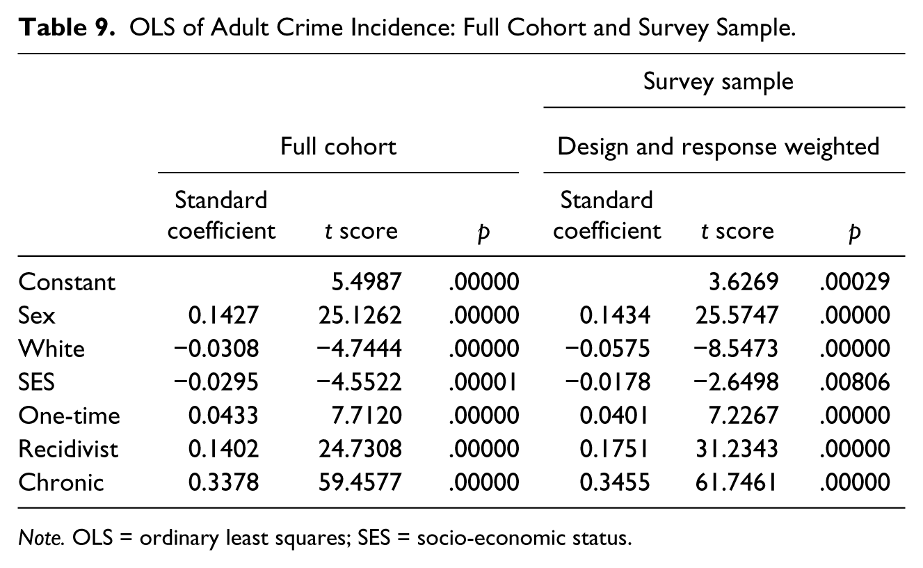
Ultimately, these descriptive statistical comparisons can only take us so far. The ultimate test of the prophylactic benefit of weighting the sample data remains to be tested using multivariate models in which the true population relationships and scores are compared with the sample estimates. These results are reported in Tables 8 and 9.
OLS of Adult Crime Incidence: Full Cohort and Survey Sample.
Note. OLS = ordinary least squares; SES = socio-economic status.
Table 8 shows a multiple logistic regression model which predicts adult crime status (prevalence; no vs. yes) using four main effects (predictor variables that were found to be strongly associated with adult crime status) and one interaction effect (sex × race/ethnicity) that was also found to have significant predictive power. For the full cohort, all of the predictor variables, sex, race/ethnicity, SES, and delinquency status, had highly significant coefficients and strong predictive efficiency (odds ratios) in classifying cases as adult criminals. When we examine the interview sub-sample with adjusted weights, the model is a good fit to the data and the results replicate very well the full cohort results. All the predictor variables are significant and strongly associated with adult crime status, although the coefficients and odds ratios are slightly different owing to sampling error (not bias).
Table 9 shows an ordinary least squares (OLS) regression model which predicts the quantitative version of the criterion measure (incidence; number of adult crimes) using four main effects (sex, race/ethnicity, SES, and delinquency status) that were found to have significant predictive power. For the full cohort, all of these predictor variables had highly significant regression coefficients (standardized βs) in explaining the variation around the number of adult crimes. As was the case for Table 9, when we examine the interviewed sub-sample, the results nicely replicate the full cohort results. Once again, all the predictor variables are significantly associated with adult crime status, although the coefficients are slightly different owing to sampling error (not bias).
Conclusion
Despite rigorous effort to locate survey respondents that have been sampled, unit non-response affects survey methodology. The 1958 Birth Cohort Follow-Up study was no exception to the rule that some drawn sampled respondents either could not be located or refused to participate. We investigated the nature of the non-response and found that there were no systematic biases in cases that could be located and interviewed versus those that could not. We then investigated whether the sampled cases exhibit a good representation of the full birth cohort. We found that the unweighted survey data were not generalizable well to the full cohort. We then applied a two-stage weighting procedure to address this problem. First, we used design weights to handle the differential selection probabilities of our disproportionate, stratified sampling design. Second, we then applied adjusted weights to address the unit non-response across the 26 ample strata. This two-stage weighting procedure has succeeded in providing an interviewed sample of the cohort which nearly perfectly represents the full birth cohort.
Footnotes
Declaration of Conflicting Interests
The author(s) declared no potential conflicts of interest with respect to the research, authorship, and/or publication of this article.
Funding
The author(s) received no financial support for the research, authorship, and/or publication of this article.