
Abstract
Many crime datasets often display an excess of “1” counts, arises when arrested criminals have the desire and ability to avoid subsequent arrests. In this study, a new Horvitz–Thompson (HT) estimator under one-inflated positive Poisson–Lindley (OIPPL) distribution which allow for one-inflation and the existence of heterogeneity in the data is developed to estimate the hidden population size of criminals. From the simulation study and applications to real crime datasets, the OIPPL is capable to provide an adequate fit to the datasets considered and the proposed HT estimator is found to produce a more precise estimate of the population size with a narrower 95% confidence interval as compared to several other contending estimators considered in this study.
Keywords
Introduction
The history of studies on estimating the population size can be detected as early as the 1600s by John Graunt (Hald, 2003) and the 1800s by Pierre Laplace (Cochran, 1978). As described by White et al. (1982), one of the earliest estimators for the population size can be traced back to the works in the late 19th, known as the Petersen–Lincoln estimator, which equates the proportion of marked sample from the recaptured sample with the proportion of the captured sample from the population. This estimator is proposed in the name of Peterson and Lincoln, two persons who had made a great contribution in the area of ecology. Chapman (1951) modified the biased Petersen–Lincoln estimator to be an unbiased estimator. In the 20th century, the estimation of population size is pioneered by M’Kendrick (1925) who studied the movement of people or cells which causes the transference of infectious diseases.
The determination of population size under capture-recapture framework involves considering both observed and unobserved members of the population. However, the number of unobserved members is unknown, and thus it needs to be estimated before a reliable population size is determined. The estimator of the population size based on the capture-recapture framework has been widely studied in biological science. Good (1953) pointed out that if a particular species is observed or represented
Besides Good–Turing and adjusted Good–Turing estimators, other estimators for the population size can also be found in many past studies. In the late 1980s, several estimators for different models were proposed (Chao, 1987, 1989; Zelterman, 1988). Chao (1987) proposed a minimum bound for the estimate of population size known as Chao estimator, for a model that incorporates heterogeneity of capture probability by making use of “1” and “2” counts only. However, under moment restrictions, another estimator for population size with a correction factor can be obtained, hence known as corrected Chao estimator. This corrected Chao estimator required the values of the first and the second sample moments. Chao (1989) proceeded to propose a bias-corrected Chao estimator under time-variation model for sparse capture-recapture data. In the presence of one-inflation, Chao estimator can extremely overestimate the population size (Böhning et al., 2019), and thus the authors proceeded to propose a modified Chao estimator to avoid overestimation by also incorporating the “2” and “3” counts. To ensure the estimator of population size estimator is robust, Zelterman (1988) proposed a new estimator called Zelterman estimator. The Zelterman estimator has a similar representation as the Horvitz–Thompson estimator except that the probability of “0” counts is obtained using Zelterman estimator rather than based on untruncated distribution. Besides these estimators, Chao and Lee (1992) proposed several other estimators known as Chao–Lee estimators for the population size by making use of sample coverage and coefficient of variation. Inspired by Chao–Lee estimators, Cecconi et al. (2012) introduced a new and flexible estimator, which involved simultaneous estimation of the population size, coefficient of variation and parameter in Dirichlet prior.
Several studies have proposed the estimator of species population size using a parametric approach, involving a statistical distribution or a regression model. One of the earlier works on estimating the population size using parametric approach can be traced back to the work by Edwards and Eberhardt (1967), Horvitz and Thompson (1952) as well as Nixon et al. (1967). The Horvitz–Thompson estimator, following the name of the authors, makes use of information on truncated and untruncated distributions of members in a population for estimating the population size. Edwards and Eberhardt (1967) have estimated the population size of cottontails by employing two geometric models based on the maximum likelihood estimator and the simple linear regression. The same techniques were employed in the study of Nixon et al. (1967) for the estimation of the population size of squirrels. In both studies, the geometric models give a closer approximation to the actual population size than other estimators considered. Since the Chao (1987) estimator disregards any information from counts larger than “2,” Niwitpong et al. (2013) incorporated censoring technique at “1” counts and zero-truncated geometric distribution to overcome problems in the Chao estimator. The resulting estimator, known as the censored estimator, depends only on the “1” counts. By using the ratio of successive probability, Anan et al. (2016) proposed an estimator for the population size based on Conway–Maxwell–Poisson distribution, which does not depend on the complex normalizing constant term in the Conway–Maxwell–Poisson distribution. The same group of authors, Anan et al. (2019) recently introduced a Good–Turing-type estimator under geometric distribution and found that the population size estimated using the new estimator will always be greater than those obtained from the Good–Turing estimator.
Several positive or zero-truncated models, which are inflated at “1” counts, have recently attracted several researchers (Godwin, 2017, 2019; Godwin & Böhning, 2017; Kaskasamkul & Böhning, 2018) because of an extra inflation parameter in the count data which captures the effects on “1” counts. Godwin and Böhning (2017) pointed out that the excess of “1” counts appears naturally when the captured and marked subjects have the inclination and the ability to avoid getting recaptured. It is important to note that the information on how to avoid being recaptured are already present and not learned after the first capture (Godwin & Böhning, 2017). The authors then proposed a Horvitz–Thompson estimator for the population size based on a one-inflated positive Poisson model, for describing the positive count data with an excess of ones. Following the work of Godwin and Böhning (2017), Godwin (2017) proposed another model that can incorporate both one-inflation and unobserved heterogeneity, known as one-inflated zero-truncated negative binomial. Recently, Godwin (2019) estimated the population size by making use of the one-inflated positive Poisson mixture model. The one-inflated positive Poisson mixture model also takes into account of both unobserved heterogeneity and excess ones when estimating the population size. Kaskasamkul and Böhning (2018) studied the zero-truncated one-inflated geometric model in estimating population size of criminals. The model assumes that the inflation parameter is imposed to all counts including “0” counts, with truncation at zero happening later (Kaskasamkul & Böhning, 2018). The authors have also considered obtaining estimates by truncating singletons completely (Kaskasamkul & Böhning, 2018). When the truncated count data are inflated or deflated at any points in the count data, one can refer to the work of Böhning and Ogden (2020) for the statistical inference as well as for estimating the size of the hidden population.
The capture-recapture technique applied in the area of biological science has also been applied for research in the field of quantitative criminology. Capture-recapture framework in the context of criminology can be described as the number of times a person initially get caught by the authorities (capture) and get caught again (recapture, if any). The idea of estimating the population size of a species can be applied in estimating the population size of criminals for a specific crime. Rossmo and Routledge (1990) stressed the importance of knowing the population size of criminals because it may affect the formulation and development of criminal justice policy. The authors proposed a model that incorporates heterogeneity in the form of inverse Gaussian and target response.
Another way of incorporating heterogeneity is by employing the truncated regression model. A group of researchers has employed the truncated Poisson regression model in estimating the population size of criminals who committed illegal firearm possession and drunk driving (Van der Heijden et al., 2003a), illegal immigrants (Van der Heijden et al., 2003b) as well as domestic violence (Van der Heijden et al., 2014). Mixtures of truncated Poisson can also be used in estimating the number of population size, as shown in the work of Böhning et al. (2004) in which the number of drug users is estimated. Besides truncated Poisson regression and truncated Poisson mixtures, truncated negative binomial regression model which can be used to explain additional unobserved heterogeneity was also applied in determining the population size of opiate users (Cruyff & Van der Heijden, 2008) and domestic violence (Van der Heijden et al., 2014). The estimated population size based on the truncated Poisson regression model can be used as a lower bound for the true population size (Van der Heijden et al., 2014). Bouchard et al. (2019) innovatively used the number of arrests in their regression models based on covariate-adjusted models and the resulting estimates refer to those who are at risk of arrest. The authors have only considered the case with the sample data consist of the number of arrests with rearrests happen in the next 5 days after the initial or previous arrests (Bouchard et al., 2019). The size and the trend of the crimes can also be estimated by evaluating the effect of individual covariates on the probabilities of survival and capture for an open population using Cormack–Jolly–Seber model (Cai & Xia, 2018).
We note that the Poisson assumption only holds if the Poisson parameter which indicates the number of arrests experienced by an individual criminal remains constant over time and assumed to be not influenced by the prior apprehension by the authority. However, this assumption is too restrictive and does not allow for extra flexibility in the data to take into account of the presence of heterogeneity and contamination (Godwin & Böhning, 2017). Our proposed model deals one form of heterogeneity which is one-inflation. We note that the one-inflation may happen from two scenarios. First, the first-time offender has the ability and desire to avoid being re-apprehended. In some cases, the offender may already have either the ability or the desire to avoid being re-apprehended (Godwin & Böhning, 2017). However, the knowledge which gives the offender the ability or desire to avoid re-apprehension may be learned prior to the first apprehension. For example, by targeting pre-offenders before their first offense in child sexual abuse (Levine & Dandamudi, 2016). Even if the offenders involved in child abuse, which is not the original intention of the prevention program, there is a chance they will stop doing after the first apprehension based on the knowledge they learned from the program. In prostitution crime, Rossmo and Routledge (1990) have noted that the prostitutes gain some knowledge from other prostitutes on how to avoid getting arrested. Surely, if they are being arrested the first time, based on Rossmo and Routledge (1990), there is high chance that they will only be arrested for one time, contributing to large number of single arrests.
Secondly, the apprehensions of the previously arrested offenders are misclassified as their first offence or into different category. Albeit being rare, this misclassification may happen due to clerical error or data collection. The police may have misclassified the criminal offenses intentionally or accidentally which then causes over or undercounting for certain offenses, which further leads to inflation or deflation (Nolan et al., 2011). For example, the uniform crime report defines robbery as a combination of assault and larceny. So, there is a chance that the robbers are wrongly charged with either assault or larceny, showing how a misclassification happens (Nolan et al., 2011).
The type of the population, whether it is open or closed is another issue that should be considered when estimating the population size of criminals. Closed population ensures the number of criminals to be constant, but this is not the case most of the time (Van der Heijden et al., 2003a). The size of the whole population may be constant but the population of the offenders is open in the sense that the offenders may enter and leave the population. New offenders enter the population by becoming first-time offenders whereas current offenders are considered as leaving the population if they are incarcerated. It is worthy to note that the new offenders who exit the population after the first arrest can also contribute to one-inflation. Therefore, it is acceptable to assume that the population are open.
The information on the behavior of criminals is not easily obtainable especially when dealing with secondary data because not all information is disclosed. For a given period of study, an open population will allow new or previously arrested offenders (outside of the period of study) to enter. The question that arises here is whether apprehension of the previously arrested offenders is categorized as the first offense. If this is the case, then we can expect misclassifications in the criminal counts. The misclassification will not happen for new offenders who commit one or multiple offenses in the period of study. If the apprehension of the previously arrested offenders is categorized based on the total number of offenses including those from outside of the period of study, then the conclusion made from the study cannot be fully explained for that particular period of study, which further complicate the statistical analysis.
When modeling count data, one important property that needs to be taken into account is overdispersion. Wagh and Kamalja (2018) mentioned that overdispersion in the data can be caused by either the existence of heterogeneity in the population or excess of zeroes. For positive count data, the “0” counts are unobserved and the majority of the data comes from “1” counts. Therefore, it is believed that an excess of “1” counts can contribute to the dispersion (over or under) in the data. Hence this paper is motivated by the need for a model that can handle dispersion which occurs due to heterogeneity in the data as well as the excess of “1” counts. The population of interest is assumed to be open with the existence of heterogeneity and large number of ones. It is believed and will be demonstrated based on the simulation study as well as real data applications that the model is pertinent for describing the population with those characteristics mentioned.
In this study, the positive Poisson–Lindley model inflated at “1” will be developed. Note that the positive Poisson–Lindley distribution, which is also known as zero-truncated Poisson–Lindley distribution, is able to adequately fit either overdispersed or underdispersed data (Ghitany et al., 2008). In other words, the positive Poisson–Lindley distribution can be thought of as a truncated Poisson count, which is adjusted for Lindley-wise distributed heterogeneity. When the inflation factor is imposed on positive Poisson–Lindley, an inflated positive Poisson–Lindley is produced that can accommodate both excess in “1” counts and heterogeneity in the data, and thus is believed to provide a better estimate for the population size.
Firstly, the positive Poisson -Lindley model inflated at “1” is developed and the maximum likelihood estimators for the parameters of the model are described. Next, the variance of the proposed estimator is derived, along with notes on some alternative estimators available in the literature. A simulation study is conducted to compare the performance of the proposed population size estimators with several other estimators. In addition, the performance of the proposed estimator in estimating the population size of criminals for two crime datasets are investigated. Finally, some remarks on the proposed model as well as the proposed estimator for the population size are discussed.
Excess “1” Counts in Positive Poisson-Lindley Distribution
There are two ways to introduce extra “1” counts into any positive count data distribution. First, the inflation parameter
One-Inflated Positive Poisson–Lindley (OIPPL) Distribution
Let

where
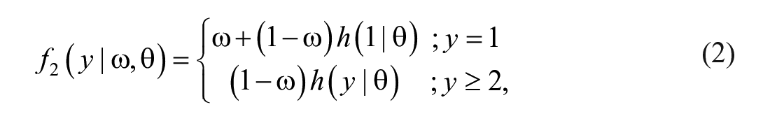
where
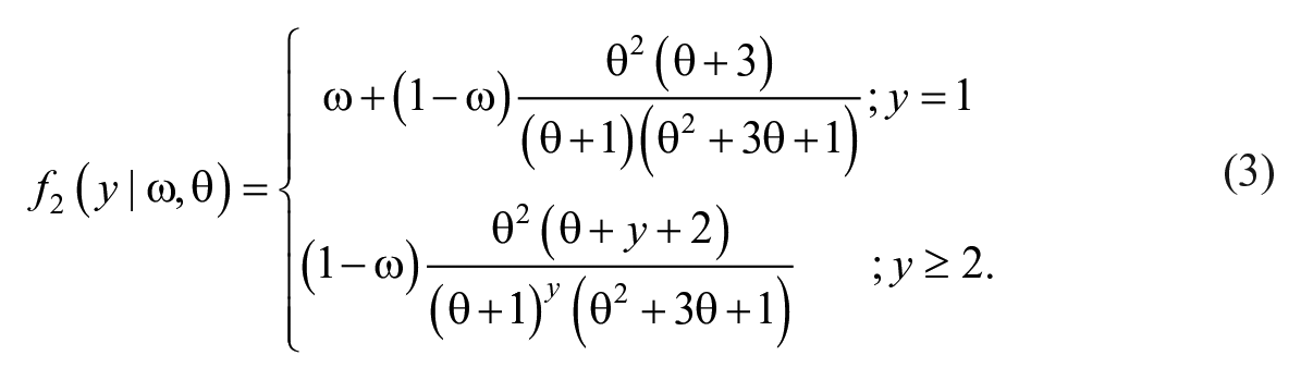
In order for OIPPL to cater for deflation as well,

where
where
It can be noted that by using the reparameterization in equation (5), a new distribution named positive one-inflated Poisson-Lindley distribution can be obtained.

However, describing the new distribution using the reparameterization in equation (5) is beyond the scope of this study. One can refer to Godwin and Böhning (2017) for the development of positive one-inflated Poisson distribution using reparameterization for one-inflated positive Poisson distribution based on a similar idea.
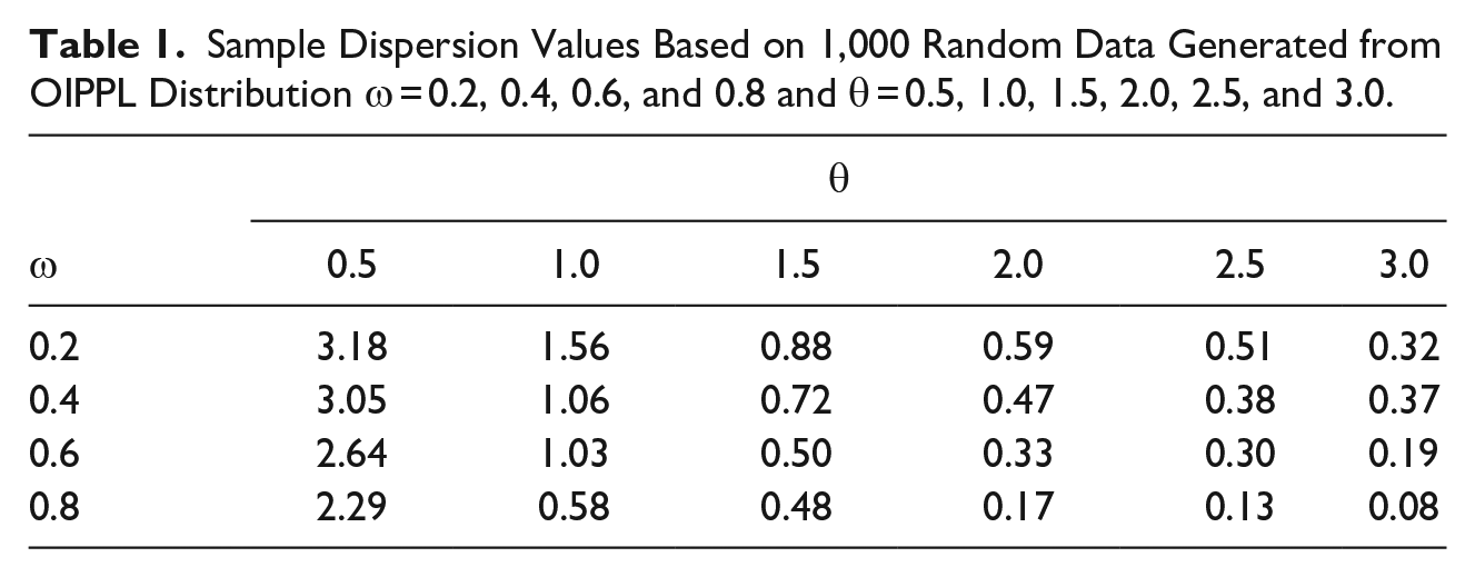
The OIPPL distribution can cater for overdispersed or underdispersed data, however, obtaining the exact dispersion index is somewhat tedious. Therefore, the sample dispersion index is calculated by taking the ratio of sample variance to the sample mean based on generated random data that follows OIPPL distribution with different values of parameters, which is given in Table 1 (see steps 1-3 in the algorithms for the first simulation study). From Table 1, it is clear that OIPPL distribution can cater for both overdispersed and underdispersed data. As
Sample Dispersion Values Based on 1,000 Random Data Generated from OIPPL Distribution ω = 0.2, 0.4, 0.6, and 0.8 and θ = 0.5, 1.0, 1.5, 2.0, 2.5, and 3.0.
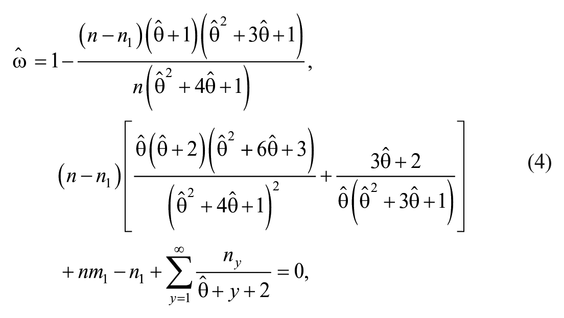
Estimation of Population Size using OIPPL Distribution
The common estimator of population size,

where
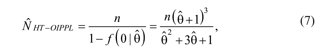
and hence can be denoted as Horvitz–Thompson estimator under OIPPL distribution (HT-OIPPL). In the context of criminology, for instance, the probability of “0” counts estimated from the untruncated distribution may explain the proportion of criminals who is yet to get caught by the authorities. The resulting estimated population size explains the total number of criminals of a specific crime in the interested area of study. In the presence of one-inflation, Böhning and Van der Heijden (2019) stressed the importance of only up-weighting the nonextra-singletons and proceeded to solve by removing the singletons completely when estimating the hidden population size. However, for example, in the drunk driving crime, the offenders may be incarcerated due to drunk driving which makes them exit the population. It is even worse if accidental deaths involve and the offenders are charged with murder but not driving under influence, which can lead to one-inflation. Therefore, with these fair assumptions, it is reasonable to keep the singletons in model fitting and the estimated parameter
Variance Estimation and Confidence Interval
A simple and general formula for the variance of the population size estimator has been proposed by Böhning (2008), which makes use of the idea that the variance of the population size estimator comes from two sources of variation. The first term in equation (8) explains the binomial variation involved in sampling

From equation (8), it is clear that the variation in the estimated population size consists of two sources of variation (Böhning, 2008). Consider the first term and by using the delta method,

Since
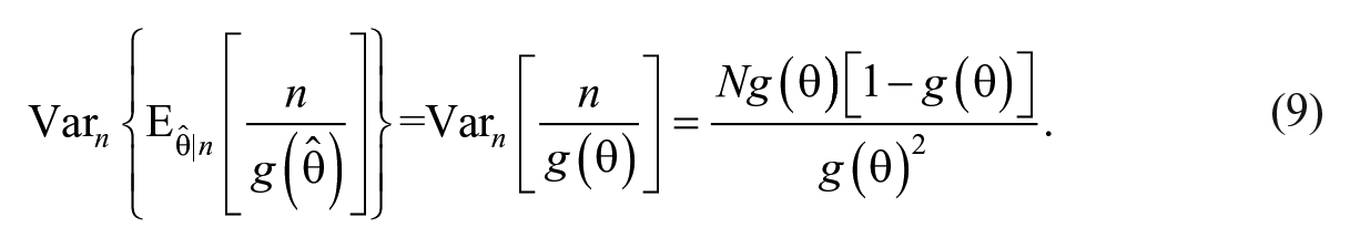
The term in equation (9) can be further estimated by substituting
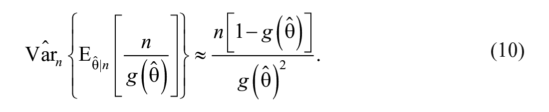
For OIPPL distribution,
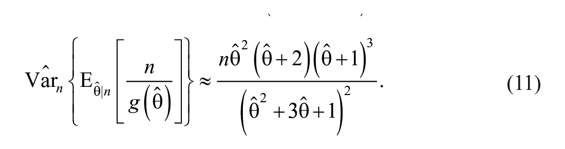
Consider the second term in equation (8), assume that

Note that by using the delta method,
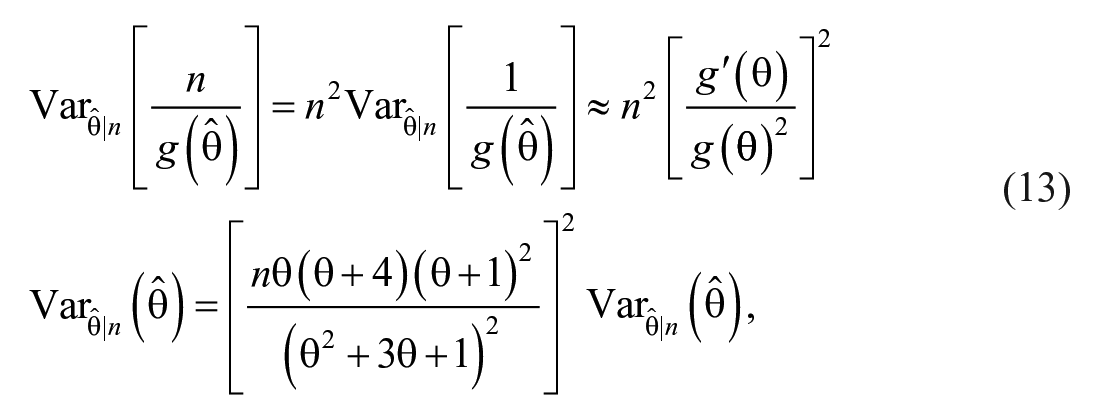
where
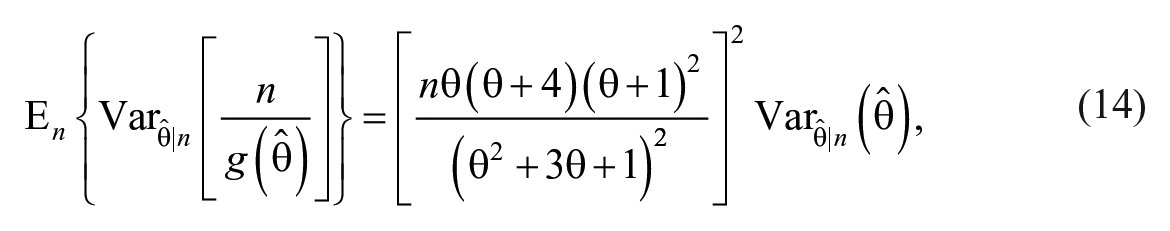
where
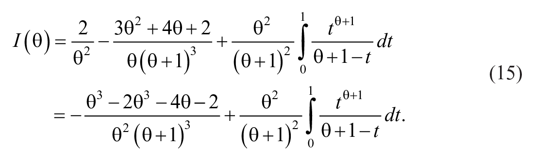
By substituting
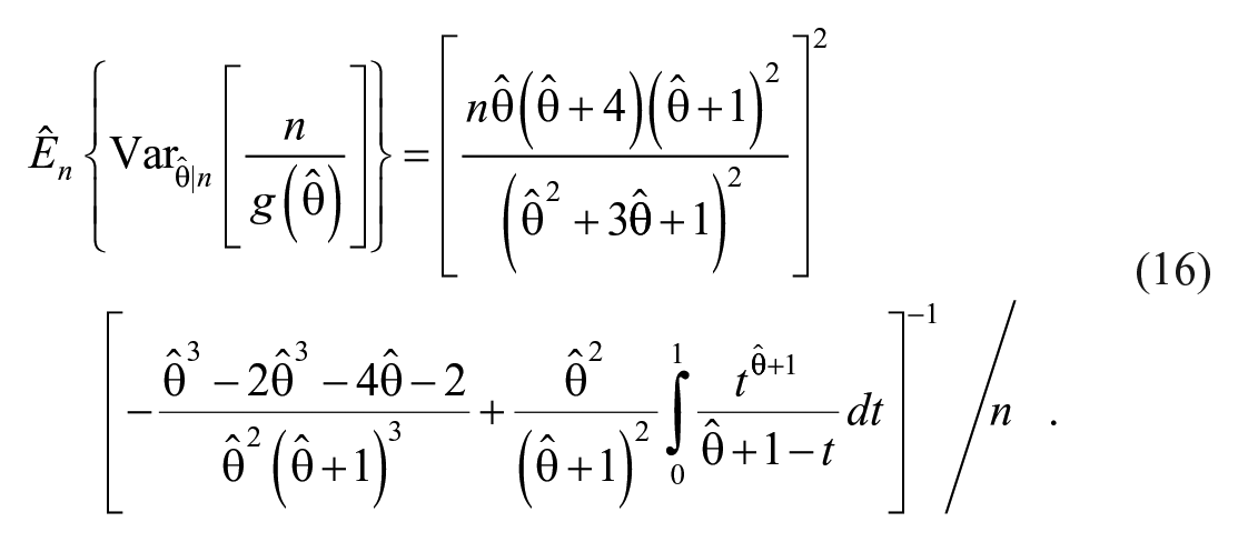
Therefore, the estimated variance of the population size estimator after some simplification and by combining equations (11) and (16), can be written as
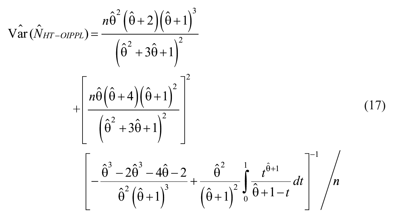
Under the assumption that the population distribution is approximately normal, a 95% confidence interval for this estimator can be obtained by using

where
Alternative Estimators
Several estimators for the population size have been introduced in the context of the capture-recapture framework but the following estimators are prioritized. Generally, the estimator and its variance are given to ease the calculation of a 95% confidence interval which has a similar form as in equation (17).
Horvitz–Thompson via zero-truncated Poisson–Lindley
A Horvitz–Thompson estimator based on zero-truncated Poisson–Lindley (HT-ZTPL) will serve as a benchmark which can be defined as

where
Good–Turing estimator
Good (1953) proposed a Good–Turing estimator (GT) for the population size which can be obtained by considering Poisson distribution as the underlying distribution. The estimated probability of zero event can be written as

with variance (Lerdsuwansri, 2012)

Zelterman estimator
Zelterman estimator (Zt) is a robust estimator for the population size under unobserved heterogeneity which can be obtained by considering truncated Poisson distribution as the underlying distribution (Zelterman, 1988). The estimator can be written as

The estimated variance for the estimator above has been studied by Böhning (2008) and is given as
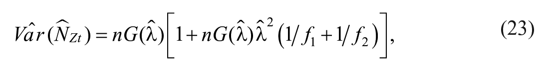
where

Chao estimator
Chao (1987, 1989) proposed Chao estimator for population size under unobserved heterogeneity where the data is generated from a Poisson mixture distribution which can be written as

with its variance studied by Böhning (2008), given as
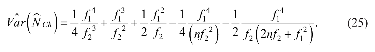
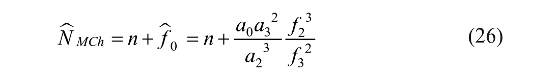
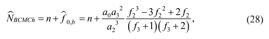
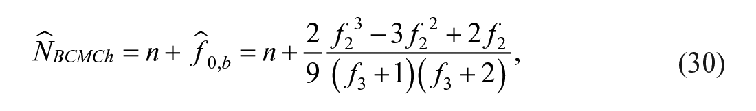
To avoid overestimation for the population size in the presence of one-inflated data, a modified Chao estimator has been proposed by Böhning et al. (2019) by excluding information of one-valued observations. The modified Chao estimator (MCh) and its variance is given by
and

respectively, where
with variance of

which is equivalent to the estimated variance of bias-corrected modified Chao estimator,
by taking
Simulation Study
A comprehensive assessment of the proposed estimator for the population size, HT-OIPPL is investigated via simulation study by comparing the performance of the estimator with some known estimators as described in Section 2.4 which are HT-ZTPL, GT, Zt, and BCMCh estimators. The bias-corrected modified Chao estimator is chosen instead of the conventional Chao estimator and the modified Chao estimator as the first is an improved estimator that considers one-inflation in the data as well with the reduction in bias. Our simulation study compares the performance of all estimators under different underlying conditions with respect to sample sizes as well as different parameter combinations in data-generating processes.
Simulation Scenario
The simulation study is conducted to investigate in which conditions, the proposed estimator is the most suitable. The data are generated from OIPPL distribution with parameters
Step 1: Generate small random data of
Step 2: Remove
Step 3: Randomly alter
Step 4: Fit the new altered count data with
Step 5: Estimate the population size based on all the estimators considered in equations (7), (19), (20), (22), and (30).
Step 6: Repeat Steps 1 to 5 for 2,000 times and obtain the estimated values of

and percentage of relative standard deviation (RSd) defined as

where
Step 7: Repeat the simulation study from the data-generating process for
Step 3 is an important step when generating OIPPL distribution because this step shows how a one-inflation occurs. It can be that the offenders exit the population due to incarceration or the rare phenomenon of misclassifying the offenders. The relative absolute bias measures how close the estimated population size from each replication to the actual population size whereas the relative standard deviation measures how close each estimated population size for each replication with each other and with respect to the actual population size. It is important that the estimated population size is close to the actual population size. The lower standard deviation value concludes that the estimator is consistent because the estimated population size from each replication has a similar value.
The results of the simulation are plotted in Figures 1 and 2. Figure 1 refers to the graph of relative absolute bias values of the estimated population size under different estimation methods with varying parameters values. Figure 2 refers to the graph of relative standard deviation values of the estimated population size under different estimation methods with varying parameters values.
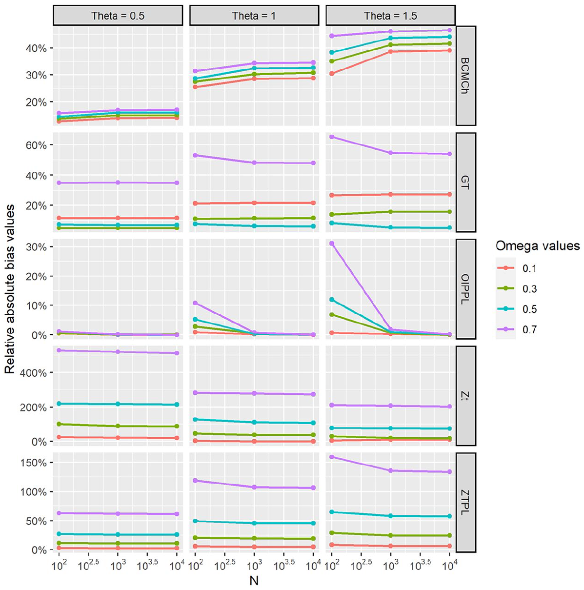
Graph of percentage relative absolute bias values of HT-OIPPL, HT-ZTPL, GT, BCMCh, and Zt estimators with respect to N = 100, 1,000, 10,000 when the data-generating process is OIPPL for parameters ω = 0.1, 0.3, 0.5, and 0.7 and θ = 0.5, 1.0, and 1.5.

Graph of percentage relative standard deviation values of HT-OIPPL, HT-ZTPL, GT, BCMCh, and Zt estimators with respect to N = 100, 1,000, and 10,000 when the data-generating process is OIPPL for parameters ω = 0.1, 0.3, 0.5, and 0.7 and θ = 0.5, 1.0, and 1.5.
From both Figures 1 and 2, it can be observed that for any given values of
Alternative Scenario
Both one-inflated positive Poisson (Godwin & Böhning, 2017) and one-inflated zero-truncated negative binomial distributions (Godwin, 2017) have similar inflation parameter

where
Step 1: Generate small random data of
Step 2: Remove
Step 3: Fit the new altered count data with
Step 4: Estimate the population size based on estimators considered in equations (7) and (31).
Step 5: Repeat Steps 1 to 4 for 2,000 times and obtain the estimated values of
Step 6: Repeat the simulation study from data-generating process for
The results of the simulation are plotted in Figures 3 and 4. Figure 3 refers to the graph of relative absolute bias values of the estimated population size under different estimation methods with varying parameters values. Figure 4 refers to the graph of relative standard deviation values of the estimated population size under different estimation methods with varying parameters values.

Graph of percentage relative absolute bias values of HT-OIPPL and HT-ZTNB with respect to N = 100, 1,000, and 10,000 when the data-generating process is ZTNB distribution for parameters λ = 1.0, 2.0, and 3.0 and α = 0.5, 1.0, and 1.5.
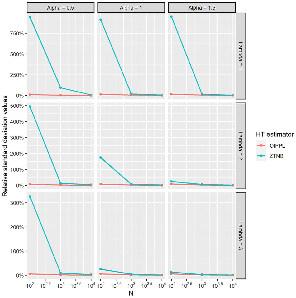
Graph of percentage standard deviation values of HT-OIPPL and HT-ZTNB with respect to N = 100, 1,000, and 10,000 when the data-generating process is ZTNB distribution for parameters λ = 1.0, 2.0, and 3.0 and α = 0.5, 1.0, and 1.5.
From Figures 3 and 4, it is not surprising that for any given
Applications
To illustrate the capability of the OIPPL distribution in model fitting, two real crime-related datasets are examined. For both datasets, we have compared the fitted number of ones from ZTPL with the original data. Since the estimated number of ones based on ZTPL is lower than the observed number of ones in the data, we have concluded that one-inflation exists in the data with respect to ZTPL distribution. The same conclusion can be reached if the score test proposed by Godwin and Böhning (2017) is used. However, the score test requires the maximum likelihood estimator of
Prostitutes in Vancouver
Rossmo and Routledge (1990) have estimated the data on street prostitutes in Vancouver by including both target response and auxiliary information. Apprehending prostitutes has a minute deterrence effect (Rossmo & Routledge, 1990), and thus it is reasonable to assume that the contagion effect is negligible. Furthermore, the authors mentioned that the prudent ones learn how to avoid being arrested and not to avoid prostitution from the experienced which will result in a large number of one-time arrest data. The prostitutes may already have the desire to avoid being arrested, but the ability to avoid learned by some prudent ones from the experienced is prior to apprehensions (Godwin & Böhning, 2017). Since the avoidance ability is not learned after the first arrest, it is reasonable that the ability will not be learned after the next arrests, which will contribute to one-inflation (Godwin & Böhning, 2017). Therefore, it is acceptable to estimate the population size of the street prostitutes in Vancouver using the OIPPL model which takes one-inflation component into account.
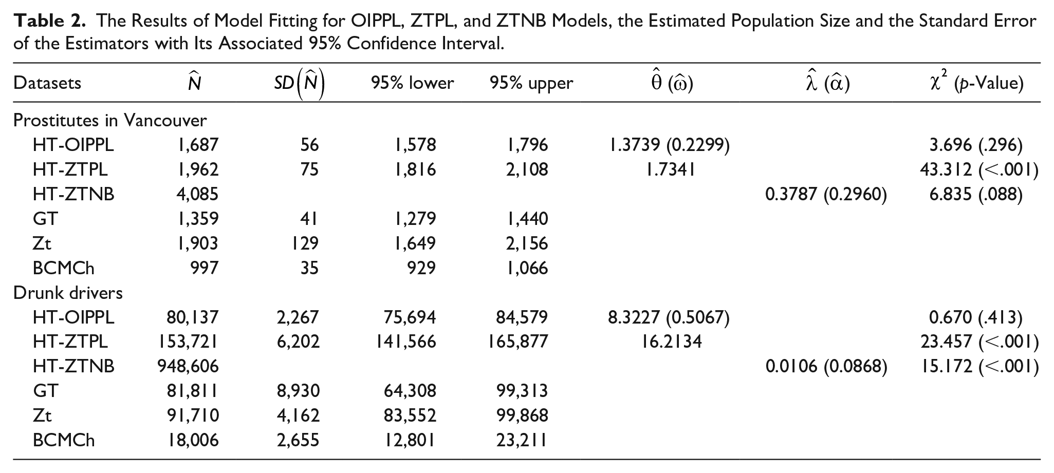
The results of the model fitting of the number of times the prostitutes get arrested and the estimated population size are given in Table 2. From the model fitting in Table 2, the OIPPL provides an adequate fit to the data along with ZTNB. However, the chi-square statistics based on fitting OIPPL is smaller than that for ZTNB, making population size estimated from HT-ZTNB less favorable than the HT-OIPPL. Furthermore, the standard deviation of all estimators except for the Zelterman estimator is considerably small. Therefore, relying solely based on the values of the standard deviation is not wise for this dataset, and consequently making HT-OIPPL the most suitable. The population size of the prostitutes in Vancouver based on HT-OIPPL is estimated to be 1,687 with a 95% confidence interval of 1,578 to 1,796. This estimate has an extremely narrower confidence limit compared with the work of Rossmo and Routledge (1990), who have estimated the population size of prostitutes in Vancouver as 1,610 with a 95% confidence interval of 1,380 to 2,000, implying that the OIPPL model improved the estimation of the population size of the prostitutes in Vancouver, at least in terms of standard error.
The Results of Model Fitting for OIPPL, ZTPL, and ZTNB Models, the Estimated Population Size and the Standard Error of the Estimators with Its Associated 95% Confidence Interval.
Drunk Drivers
Police records on drunk drivers have been considered by Van der Heijden et al. (2003) to estimate their population size. The authors have employed both the zero-truncated Poisson null model and regression model in estimating the population size of drunk drivers. The unobserved heterogeneity in the data is explained by adding covariates in the regression model (Van der Heijden et al., 2003). Godwin and Böhning (2017) have eliminated the contagion factor due to police because the police stop and check each passing driver and arrest those who are drunk driving. Besides, when drunk drivers are locked up, they exit the population for some time and this will contribute to one-inflation in the arrest data. On that account, the OIPPL model is a suitable candidate for modeling data on drunk drivers with a large number of ones and consequently, for estimating the population size.
The results of the model fitting of the data and the estimated population size are given in Table 2. It is found that the OIPPL model provides an adequate fit to the data, whereas ZTPL and ZTNB fail to adequately fit the data. The population size estimated from the HT-OIPPL can be compared directly with the population size estimated based on the null model from Van der Heijden et al. (2003). The authors have provided an estimate of 78,710 with a 95% confidence interval of 72,738 to 84,682 for the population size. From our proposed model, the estimated population size is 80,137 with a tighter 95% confidence interval of 75,694 to 84,579. The authors did mention that the lower bound of the estimated population size of drunk drivers is 113,771 because the added covariates to the zero-truncated Poisson regression reduce the deviance of the model significantly (Van der Heijden et al., 2003). However, since the OIPPL model gives a better estimate for the population size of drunk drivers against the null model from Van der Heijden et al. (2003) in terms of standard error and confidence interval, it is presumed that the regression model based on the OIPPL will improve the lower bound of the population size. This hypothesis is something to be tested in future study. Even though the BCMCh estimator has a relatively close standard deviation to HT-OIPPL and a significantly smaller estimated population size, these values are questionable because its validity cannot be tested statistically, unlike the estimated population size based on OIPPL, in which the chi-square goodness-of-fit test is performed as a model adequacy test. Other considered estimators give very high standard error making them less desirable when selecting the best estimator for the population size of drunk drivers.
Conclusions
In many cases, the hidden population size is unknown and needs to be estimated. In criminology, knowing the population size of criminals for a crime is important in establishing and formulating new rules. A new distribution which is named as one-inflated positive Poisson–Lindley distribution is proposed and the new distribution incorporates the one-inflation component which is a form of heterogeneity that exists when the data has a large number of “1” counts. The flexibility of this distribution can be seen when the datasets generated randomly from this distribution has the property of either overdispersion or underdispersion, together with a large number of ones in the data.
In order to estimate the hidden population size, a new estimator for the population size that takes the form of Horvitz–Thompson estimator is proposed by considering the one-inflated positive Poisson–Lindley distribution as the underlying model. The performance of this new estimator is investigated in the context of unbiasedness and consistency, with comparison to other commonly used empirical estimators such as Good–Turing estimator, bias-corrected modified Chao estimator and Zelterman estimator. Horvitz–Thompson estimator based on zero-truncated Poisson–Lindley, also known as positive Poisson–Lindley is also included in the simulation study for comparison purposes. It is not surprising that when the simulated data are generated with an assumption that the data follow the proposed model, the estimated population size is closer to the original values, which can be seen from the small values of percentage of relative absolute bias and percentage of relative standard deviation. Therefore, the proposed estimator is asymptotically unbiased and consistent.
To exhibit the usefulness of the proposed estimator under different data-generating process, the zero-truncated negative binomial distribution is selected because the distribution has neither one-inflation component nor heterogeneity in the form of Lindley distribution. The performance of the proposed estimator is compared with the Horvitz–Thompson estimator based on the zero-truncated negative binomial distribution. It is expected that the latter estimator gives better estimates when the zero-truncated negative binomial distribution is selected as the data-generating process. However, for small sample size, the proposed estimator gives a lower percentage of relative absolute bias, suggesting that the proposed model is useful with small sample generated from the zero-truncated distribution. Furthermore, the percentage of relative standard deviation of the proposed estimator is always low than those from the Horvitz–Thompson estimator based on the zero-truncated negative binomial distribution, suggesting a consistent estimation over different sample sizes. Therefore, it can be concluded that it is harmful to ignore the use of the proposed estimator under different data-generating process.
Two datasets with a large number of ones are used for model fitting to investigate the performance of the proposed estimator in estimating the population size of real crime datasets. The results of the model fitting to the two datasets show that the proposed model is adequate in describing the data. The standard deviation of estimated population size based on the OIPPL for all datasets is found to be considerably small when compared to other estimators and this results in a narrower 95% confidence interval. The estimated population size can be a useful indicator for authorities to understand the scale of criminals who have not been apprehended yet. In reality, the real population size is still unknown and it is believed that the estimated population size can be set as a starting value for the true population size.
In some cases, the criminals do learn to avoid after the initial arrest and the deterrence will affect the probability of re-apprehension. In this case, our model may not be able to fully capture the effects of the deterrence, which is a form of contagion. An in-depth analysis can also be done to further understand the behavior of the criminals by incorporating demographic, economic and social factors as covariates into a regression model, which can be further investigated in the future study. Some covariates that can be included are age, gender, race, education, poverty, involvement in a gang violence and others. The covariates vary based on the crime of interest. By selecting appropriate factors into the regression model, a better view of the physical behavior of the criminals for a specific crime in a society can be obtained, and this will provide a more accurate estimation of the population size.
Footnotes
Declaration of Conflicting Interests
The author(s) declared no potential conflicts of interest with respect to the research, authorship, and/or publication of this article.
Funding
The author(s) disclosed receipt of the following financial support for the research, authorship, and/or publication of this article: This research is funded by Ministry of Education, Malaysia, grant number FRGS/1/2019/STG06/UKM/01/5 and by Universiti Kebangsaan Malaysia, grant number GUP-2019-031.