On Direction of Dependence in Latent Variable Contexts

Abstract

Approaches to determining direction of dependence in nonexperimental data are based on the relation between higher-than second-order moments on one side and correlation and regression models on the other. These approaches have experienced rapid development and are being applied in contexts such as research on partner violence, attention deficit hyperactivity disorder, and currency exchange rates. In this article, we propose using these methods in the context of latent variables analysis. Specifically, we propose creating component or factor scores and relating the component score or factor score variables to each other by using methods for the determination of direction of dependence. Empirical examples use data from the development of aggression in adolescence. In the discussion, issues concerning the establishment of causal relation in empirical research are addressed.

Keywords

direction of effects latent variables PCA SEM

In nonexperimental research, the direction of dependence, also called the direction of effects, is not always obvious. For example, Dodge and Rousson (2001) asked which of the world currencies affects others to increase or decrease in value. Nigg et al. (2008) asked whether an increased blood lead content is the cause for attention deficit hyperactivity disorder or whether attention deficit hyperactivity disorder has the effect that children expose themselves more often to lead-tainted objects. von Eye and DeShon (2012) asked whether intimate partner violence has the effect that the victims turn depressive or whether depressive individuals are more likely to become victims of intimate partner violence.

In the context of methods of analysis of manifest variables, there have been approaches to statistically identify the directional dependence that are based on third- and fourth-order moments of the observed variables (e.g., Dodge & Rousson, 2001; Dodge & Yadegari, 2010; Sungur, 2005; von Eye & DeShon, 2008, 2012). The idea that carries these methods is discussed in the context of a valid linear regression model. The idea is that the distribution of an observed dependent variable, Y, is a convolution of the distribution of an independent variable, X, that can be nonnormally distributed, and the normally distributed residual. Because this residual is added to X, the distribution of the dependent variable, Y, is necessarily closer to a normal than the distribution of Y without the effect of X. Measures of skewness and kurtosis can be employed to compare the skewnesses of X and Y, or of Y with and without the presence of X.

Two additional approaches to the analysis of directional dependence have been discussed, both in the context of an analysis of manifest variables. First, the direction of dependence perspective has been extended based on the third moments of linear regression residuals (Wiedermann, Hagmann, Kossmeier, & von Eye, 2013). Second, models of copula regression have been proposed to determine direction of dependence. Recent copula regression approaches use asymmetric models that allow one to also consider variable interactions (Kim & Kim, 2013).

In the context of methods of analysis of latent variables approaches to the analysis of direction dependence are scarce. The issue is either discussed in the context of causality, as, for example, by Sobel who states (1996) that the interpretation of SEM parameters as effects does “not generally hold, even if the model is correctly specified and a causal theory is given” (p. 376), or in the context of causal foundations of structural equation modeling (see, e.g., Pearl, 2012). One reason for this state of affairs is that most structural equation models use moments of first and second, but not higher order.

In the only approach to analyzing directional dependence in latent variables that is known to the authors, Shimizu and Kano (2008) proposed including higher order moment structures. The authors assume nonnormal distributions of exogenous variables. This approach can be viewed as parallel to the one proposed by Dodge and collaborators for manifest variables. The use of higher order moments is not new in structural equation modeling. It has been proposed, for example, in the context of asymptotically distribution-free, generalized least squares estimation (Bentler, 1983; Browne, 1982, 1984) and in the context of analysis of interaction effects (e.g., Jöreskog & Yang, 1996). The use of higher order moments in the context of directional dependence is unique to the work by Shimizu and Kano (2008).

In the present article, we build on these approaches and propose methods for the analysis of the direction of dependence in contexts of latent variable analysis and structural modeling. Specifically, we propose using standard latent variable models, and we propose relating latent variables from these models to each other using methods proposed for the determination of direction of dependence for manifest variables.

This article is structured as follows. First, we review an approach to determining direction of dependence in manifest variables. This review consists of two parts. In the first, we focus on correlation methods, in the second, we focus on regression methods. Second, we apply these methods to component scores from principal component analysis (PCA). Third, we apply these methods to factor scores from structural modeling.

Direction of Dependence in Manifest Variables

For the considerations in this section, we use observed, manifest variables that are nonnormal. This is typically the case in observed, specifically psychometric data. Micceri (1989) found that not one of the 400 psychometric data sets that he examined can be shown to be drawn from a normal population. Nonnormal variables have skewness or kurtosis that deviate from expectation. This characteristic will be used throughout this article. In addition to being assumed to be nonnormal, the variables discussed here are viewed in a linear regression context. Let two variables under study be X and Y. The two regression equations that can be estimated to predict these two variables from each other are

Y = β_{0, Y} + β_{1, Y} X + ϵ_{Y},

and

X = β_{0, X} + β_{1, X} Y + ϵ_{X},

where the subscripts indicate the dependent variable. The parameters β₀ refer to the model intercepts, the β₁ refer to the slope parameters, and the $ϵ$ denote the regression residuals. It is well known that standard regression analysis is not helpful when it comes to determining the direction of effects for X and Y (this was illustrated, e.g., by von Eye & DeShon, 2012). The reason for this characteristic of regression analysis is that it is based on first- and second-order moments. Higher order moments are not considered. As is also well known, correlations are symmetric and, therefore, not helpful for the determination of the direction of effect. Consider the correlation between X and Y,

ρ_{X Y} = \frac{{cov}_{X Y}}{σ_{X} σ_{Y}},

where the numerator shows the covariance of X with Y, and the denominator shows the standard deviations of X and Y. Using information from regression, the correlation between X and Y can also be expressed as

ρ_{XY} = β_{1, X} \frac{σ_{X}}{σ_{Y}} = β_{1, Y} \frac{σ_{Y}}{σ_{X}} .

However, as was shown formally by Dodge and Rousson (2001), Muddapur (2003), and by Sungur (2005), the correlation ρ_XY also has an asymmetric property if one considers the skewness of the two variables, X and Y. Specifically, the authors show that

ρ_{XY}^{3} = \frac{γ_{Y}}{γ_{X}},

where γ_X and γ_Y are the skewness coefficients of X and Y, respectively. This relation holds if γ_Y > 0 and γ_X > γ_Y, which reflects the asymmetric property of ρ_XY. Similarly, Dodge and Yadegari (2010) show that

ρ_{XY}^{4} = \frac{κ_{Y}}{κ_{X}},

where κ_X and κ_Y are the kurtosis coefficients of X and Y. As for skewness, the relation of the two kurtosis measures holds if κ_X > 0 and if κ_X > κ_Y.

Let X be hypothesized to be the explanatory variable and Y the response variable. Let both be observed in a nonexperimental study. To determine whether there is support for this hypothesis, the statistic $ρ_{XY}^{3}$ can be used. The absolute value of $ρ_{XY}^{3}$ is, by definition, less than or equal to 1. Now, consider that, as can be seen in the regression equations, Y is a convolution of a nonnormal explanatory variable and a normal residual term. From this characteristic, we can conclude that the skewness of the response variable is always smaller than the skewness of the explanatory variable. In other words, if γ_X > γ_Y, Y may be the response variable. If, in contrast, γ_X < γ_Y, X may be the response variable.

When hypotheses about directional dependence are tested, five implications of this relationship between γ_X and γ_Y are of importance (von Eye & DeShon, 2012):

Let $0 \leq ∣ ρ_{XY}^{3} ∣ \leq 1$ . Then, if a symmetric error, for example, normally distributed noise, is added to a skewed explanatory variable, the response variable will be less skewed.

The cube of the correlation coefficient can be interpreted as the percentage of skewness that is left after a linear model was applied to describe the relationship between X and Y.

If the ratio of the two skewness scores lies outside [−1; +1], the cube of the correlation suggests that Y, not X, is the explanatory variable.

If X is perfectly symmetric as is the case in normal or in uniform distributions, directional dependence cannot be determined by using the methods discussed here.

Above and beyond what is generally known about Pearson’s correlation coefficient, ρ_XY, it does, in the context of linear modeling and when variables are not bivariate normal, possess asymmetric properties.

Direction Dependence Based on Linear Regression Residuals

Recently, the directional dependence perspective has been used as a starting point to investigate properties of residuals of competing linear regression models (Wiedermann et al., 2013). Again, consider the two linear regression equations $Y = β_{0, Y} + β_{1, Y} X + ϵ_{Y}$ and $X = β_{0, X} + β_{1, X} Y + ϵ_{X}$ . Furthermore, considering the relationship

ρ_{XY}^{2} = β_{1, Y} β_{1, X},

we obtain

ϵ_{X} = (1 - ρ_{XY}^{2}) X - \frac{ρ_{XY}^{2}}{b_{1, Y}} ϵ_{Y}

for the residual term $ϵ_{X}$ . When X and $ϵ_{Y}$ are independent, the following relation holds for the third centralized moment of $ϵ_{X}$ :

E ({(\frac{ϵ_{X} - μ_{ϵ_{x}}}{σ_{ϵ_{X}}})}^{3}) = {(\frac{(1 - ρ_{XY}^{2}) σ_{X}}{σ_{ϵ_{X}}})}^{3} E ({(\frac{X - μ_{X}}{σ_{X}})}^{3}) - (\frac{ρ_{XY}^{2} σ_{ϵ_{Y}}}{b_{1, Y} σ_{ϵ_{X}}}) E ({(\frac{ϵ_{Y} - μ_{ϵ_{Y}}}{σ_{ϵ_{Y}}})}^{3}) .

Assuming symmetrically distributed residuals for the true regression model, that is, $γ_{ϵ_{Y}} = 0$ or

E ({(\frac{ϵ_{X} - μ_{ϵ_{x}}}{σ_{ϵ_{X}}})}^{3}) = {(\frac{(1 - ρ_{XY}^{2}) σ_{X}}{σ_{ϵ_{X}}})}^{3} E ({(\frac{X - μ_{X}}{σ_{X}})}^{3}),

we arrive at the following three implications:

The skewness of X and the skewness of $ϵ_{X}$ will always have the same sign.

If the remaining terms in the above equation are fixed, the skewness of $ϵ_{X}$ increases with the skewness of X.

If the remaining terms are fixed, the skewness of $ϵ_{X}$ increases as the correlation $ρ_{XY}$ decreases.

In particular, from implication (2) we can conclude that the skewness of residuals can be used for decisions on the direction of effects. That is, for the correctly specified regression model, we would assume that the null hypothesis of symmetric residuals can be retained. Conversely, for the misspecified model, we would expect the null hypothesis of symmetry be rejected.

Decision Rule. When $H_{0} : γ_{ϵ_{X}} = 0$ is rejected and $H_{0} : γ_{ϵ_{Y}} = 0$ is retained, we can conclude that $Y$ is the response variable and $X$ is the explanatory variable. If $H_{0} : γ_{ϵ_{X}} = 0$ is retained and $H_{0} : γ_{ϵ_{Y}} = 0$ is rejected, we can conclude that $Y$ is the explanatory variable and $X$ is the response variable. If both null hypotheses are rejected/retained, no distinct decision on directional dependence can be made (Wiedermann et al., 2013).

Direction Dependence in Latent Variables Contexts

When latent variables or structural models are specified, the situation can be quite similar to the one encountered for manifest variables. It is not always clear which of the latent variables, for example, principal components or factors, has the response variables as indicators and which has the explanatory variables as indicators. Therefore, a method such as the one described in section “Direction of Dependence in Manifest Variables” can be useful in the analysis of latent variables as well. In the following sections, we discuss such a method. We begin with a description of the data situation in latent variables analysis.

Component Scores

In this section, we discuss the case of principal components analysis (PCA). We first provide a brief review of those elements of PCA that we need for the calculation of component scores. The presentation follows that by Bartholomew and Knott (1999; cf. Hershberger, 2005).

Let Σ be a p×p variance–covariance matrix, Λ a p×q matrix of coefficients (loadings), and Ψ a p×p diagonal matrix of variances. Then, for q = p, the representation

Σ = ΛΛ' + Ψ

is possible, because Σ is symmetric. Σ can also be expressed as

Σ = A Θ A',

where Θ is a diagonal matrix. The elements of Θ are the eigenvalues of Σ, and A is an orthogonal matrix whose column vectors are the eigenvectors of Σ. The first equation for Σ, above, follows if Λ = AΘ^1/2 and Ψ = 0 (under the second of these conditions, PCA and principal factor analysis are equivalent).

Now, let y be the q latent variables, and let x be the p observed variables, conditionally distributed as

x ∣ y ~ N_{p} (μ + Λ y, Ψ),

where µ is a vector of constants (means, intercepts). Given that Λ = AΘ^1/2, the conditional distribution of x can be expressed as a linear combination of independent variables,

x = μ + Λ y = μ + A Θ^{1 / 2} y .

The variables

y^{*} = Θ^{1 / 2} y = A' (x - μ)

are the well-known principal components. It is standard procedure to choose the first principal component such that the explained portion of variance of x is maximized. The second principal component maximizes the explained portion of the remaining variance while being uncorrelated with the first component, and so on.

Component scores, F, indicate the coordinates of individual cases in the space of principal components. They are straightforwardly calculated as

F = Λ^{- 1} x .

The distribution of component scores depends on a number of factors, including sample size and the underlying data generation process. Component scores and factor scores are not necessarily normally distributed (for illustrations, see, e.g., Steinley & McDonald, 2007). The following considerations are based on component scores that are not normally distributed.

Component Scores and Directional Dependence

As was discussed above, third- and fourth-order moments (skewness and kurtosis) can be used to examine distributional characteristics of data. Third- and fourth-order moments are central moments (for an overview, see Walwyn, 2005). Let F be the random component score variable and k a natural number. Then, the kth central moment, aka kth order moment, is

μ_{k} = \frac{E [{(F - c)}^{k}]}{σ_{F}^{k}},

that is, the expectation of F minus a constant c, raised to the power of k. Usually, the mean is used for c. In the present context, the second, third, and fourth moments are of interest. The first moment is the sum of deviations from the mean. The second moment is the variance of F. The third moment, the skewness of F, is

μ_{3} = \frac{E [{(F - μ_{F})}^{3}]}{σ_{F}^{3}},

and the fourth moment, the kurtosis of F, is

μ_{4} = \frac{E [{(F - μ_{F})}^{4}]}{σ_{F}^{4}} - 3 .

Definition and computational aspects of central moments are covered in many textbooks (e.g., Hogg & Tanis, 1993; see also D’Agostino & Pearson, 1973).

Karl Pearson (1895) proposed that skewness and kurtosis can be used to determine whether a variable is normally distributed. Based on this proposition, two lines of research have evolved. The first involves deriving tests of (multi)normality (see, e.g., D’Agostino, 1971; D’Agostino, Belanger, & D’Agostino, 1990; D’Agostino & Pearson, 1973; Mardia, 1970, 1980; von Eye & Gardiner, 2004). The second line of research concerns the determination of direction of effects (see, e.g., Dodge & Rousson, 2000, 2001; Muddapur, 2003; Shimizu, Hoyer, Hyvärinen, & Kerminen, 2006; Shimizu & Kano, 2006; Sungur, 2005, von Eye & DeShon, 2008, 2012; Wiedermann et al., 2013).

In the following paragraphs, we review, discuss, and build on the second of these lines of work. We begin by deriving the equation $ρ_{XY}^{4} = κ_{Y} / κ_{X}$ (Dodge & Yadegari, 2010) for the situation in which component scores are used to determine which of the principal components can be interpreted as the explanatory variable. The components are the result of separate PCAs.

Let F_Y be the component score variable for the principal component that is hypothesized to take the role of the dependent variable and F_X the component score variable for the principal component variable that is hypothesized to be explanatory. Then, the correlation between these two variables is

ρ_{F_{X}, F_{Y}} = \frac{co v_{F_{X}, F_{Y}}}{σ_{F_{X}} σ_{F_{Y}}}

ρ_{F_{X}, F_{Y}} = β_{1, F_{X}} \frac{σ_{F_{X}}}{σ_{F_{Y}}} = β_{1, F_{Y}} \frac{σ_{F_{Y}}}{σ_{F_{X}}} .

The linear relationship between these two variables is

κ_{F_{Y}} = ρ^{4} κ_{F_{X}} + {(1 - ρ^{2})}^{2} κ_{ϵ}

(from here on, we again omit the subscripts of $ρ_{F_{X}, F_{Y}}$ ).

The kurtosis coefficients of F_Y, F_X, and the residual $ϵ$ are given by

κ_{F_{Y}} = \frac{E {[F_{Y} - E (F_{Y})]}^{4}}{σ_{F_{Y}}^{4}} - 3,

κ_{F_{X}} = \frac{E {[F_{X} - E (F_{X})]}^{4}}{σ_{F_{X}}^{4}} - 3,

and

κ_{ϵ} = \frac{E {[ϵ - E (ϵ)]}^{4}}{σ_{ϵ}^{4}} - 3 .

Based on the equations for the linear relationship between F_Y and F_X and the correlation between F_Y and F_X, we obtain $κ_{F_{Y}} = ρ^{4} κ_{F_{X}} + {(1 - ρ^{2})}^{2} κ_{ϵ},$ given in Equation (22) and, if κ_ε = 0,

κ_{F_{Y}} = ρ^{4} κ_{F_{X}} .

From (26), we obtain

ρ^{4} = \frac{κ_{F_{Y}}}{κ_{F_{X}}} .

Equation (27) can also be derived as follows (Dodge & Yadegari, 2010, derive this for manifest variables). Because F_X is independent of $ϵ$ ,

1 - ρ^{2} = {(\frac{σ_{ϵ}}{σ_{F_{Y}}})}^{2} .

Under expectation, we can rewrite the expression F_Y−E(F_Y) as

F_{Y} - E (F_{Y}) = β_{0, F_{X}} + β_{1, F_{X}} + ϵ - E (β_{0, F_{X}} + β_{1, F_{X}} +) = β_{1, F_{X}} (F_{X} - E (F_{X})) + (ϵ + E (ϵ)) .

In the next step, we divide Equation (29) by $σ_{F_{X}}$ and apply (28). This results in

(\frac{F_{Y} - E (F_{Y})}{σ_{F_{Y}}}) = ρ (\frac{F_{X} - E (F_{X})}{σ_{F_{X}}}) + \frac{σ_{ϵ}}{σ_{F_{Y}}} (\frac{ϵ - E (ϵ)}{σ_{ϵ}}) .

Raising (30) to the fourth power yields

\begin{matrix} E {(\frac{F_{Y} - E (F_{Y})}{σ_{F_{Y}}})}^{4} = ρ^{4} E {(\frac{F_{X} - E (F_{X})}{σ_{F_{X}}})}^{4} \\ + C_{2}^{4} ρ^{2} E {(\frac{F_{X} - E (F_{X})}{σ_{F_{X}}})}^{4} {(\frac{σ_{ϵ}}{σ_{F_{X}}})}^{2} E {(\frac{ϵ - E (ϵ)}{σ_{ϵ}})}^{2} + {(\frac{σ_{ϵ}}{σ_{F_{Y}}})}^{4} E {(\frac{ϵ - E (ϵ)}{σ_{ϵ}})}^{4}, \end{matrix}

where according to Dodge and Yadegari (2010), C = 4!(2!(4 − 2)!). After simplification and using (28) again, we obtain $κ_{F_{Y}} = ρ^{4} κ_{F_{X}} + {(1 - ρ^{2})}^{2} κ_{ϵ}$ given in Equation (22). If the residuals are normally distributed, κ_ε = 0, this expression simplifies to $κ_{F_{Y}} = ρ^{4} κ_{F_{X}}$ and we obtain, for component score variables, $ρ^{4} = κ_{F_{Y}} / κ_{F_{X}} .$ In applications in which researchers aim to determine whether F_X or F_Y is the explanatory variable, both kurtosis measures must be unequal to zero.

In a similar way, we can derive the relationship between ρ and skewness that was originally derived, for manifest variables, by Dodge and Rousson (2000). Specifically, we now raise the expression in (30) to the third power and obtain

E {(\frac{F_{Y} - E (F_{Y})}{σ_{F_{Y}}})}^{3} = ρ^{3} E {(\frac{F_{X} - E (F_{X})}{σ_{F_{X}}})}^{3} + {(\frac{σ_{ϵ}}{σ_{F_{Y}}})}^{3} E {(\frac{ϵ - E (ϵ)}{σ_{ϵ}})}^{3} .

From using (28) again, we obtain

γ_{F_{Y}} = ρ^{3} γ_{F_{X}} + {(1 - ρ^{2})}^{2 / 3} γ_{ϵ} .

If the residual is normally distributed, $γ_{ϵ} = 0$ , and we obtain $γ_{F_{Y}} = ρ^{3} γ_{F_{X}}$ and $ρ^{3} = γ_{F_{Y}} / γ_{F_{X}} .$

In applications in which researchers aim to determine whether F_X or F_Y is the explanatory variable, both skewness measures must be unequal to zero.

Interpretation. As is well known, the square of the correlation coefficient indicates the portion of variance shared by two variables, in the present case F_X and F_Y. Accordingly, ρ³ indicates the portion of skewness of F_Y that can be explained by F_X, and ρ⁴ indicates the portion of kurtosis of F_Y that is explained by F_X.

Decision rules. In parallel to the decision guidelines proposed by von Eye and DeShon (2008), we suggest the following decision rules based on the skewness of two nonnormal component score variables, F_X and F_Y:

If $γ_{F_{Y}} > γ_{F_{X}},$ the direction of effect goes from F_X to F_Y

If $γ_{F_{X}} > γ_{F_{Y}},$ the direction of effect goes from F_Y to F_X

If $γ_{F_{Y}} = γ_{F_{X}},$ the direction of effect is uncertain (if it exists)

Two approaches are available for statistical inference on $γ_{F_{X}}$ and $γ_{F_{Y}} .$ First, von Eye and DeShon (2012) proposed the use of normality tests, that is, D’Agostino’s skewness test (D’Agostino, 1971) and the procedure proposed by Anscombe and Glynn (1983) to evaluate kurtosis values. Second, for statistical inference on the difference of skewness and kurtosis estimates Pornprasertmanit and Little (2012) suggested the use of nonparametric bootstrapping.

Component Scores and Properties of the Regression Residuals

As was discussed in section “Direction Dependence Based on Linear Regression Residuals,” indicators of the skewness of linear regression residuals can be used to evaluate the direction of effects. Again, let $F_{Y}$ be the component score for the principal component of the putative response variable and let $F_{X}$ be the component score for the principal component which is expected to be the explanatory variable. In this case $F_{Y} = β_{0, F_{Y}} + β_{1, F_{Y}} X + ϵ_{F_{Y}}$ reflects the true data generating process and $F_{X} = β_{0, F_{X}} + β_{1, F_{X}} Y + ϵ_{F_{X}}$ reflects the misspecified model. Using the relationship $ρ_{F_{X}, F_{Y}}^{2} = β_{1, F_{X}} β_{1, F_{Y}},$ we can write

ϵ_{F_{X}} = (1 - ρ_{F_{X}, F_{Y}}^{2}) F_{X} - \frac{ρ_{F_{X}, F_{Y}}^{2}}{b_{1, F_{Y}}} ϵ_{F_{Y}}

for the residual term $ϵ_{F_{X}}$ . Because $F_{X}$ and $ϵ_{F_{X}}$ are assumed to be independent, the following relationship holds for the variances:

σ_{ϵ_{F_{X}}}^{2} = {(1 - ρ_{F_{X}, F_{Y}}^{2})}^{2} σ_{F_{X}}^{2} + {(\frac{ρ_{F_{X}, F_{Y}}^{2}}{b_{1, F_{Y}}})}^{2} σ_{ϵ_{F_{Y}}}^{2} .

If we insert the third centralized moments, we obtain

E ({(\frac{ϵ_{F_{X}} - μ_{ϵ_{F_{X}}}}{σ_{ϵ_{F_{X}}}})}^{3}) = {(\frac{(1 - ρ_{F_{X}, F_{Y}}^{2}) σ_{F_{X}}}{σ_{ϵ_{F_{X}}}})}^{3} E ({(\frac{F_{X} - μ_{F_{X}}}{σ_{F_{X}}})}^{3}) - (\frac{ρ_{F_{X}, F_{Y}}^{2} σ_{ϵ_{F_{Y}}}}{b_{1, F_{Y}} σ_{ϵ_{F_{X}}}}) E ({(\frac{ϵ_{F_{Y}} - μ_{ϵ_{F_{Y}}}}{σ_{ϵ_{F_{Y}}}})}^{3}) .

If we further assume that the residuals of the true linear regression model are symmetrically distributed, that is, $γ_{F_{Y}} = 0,$ we again obtain the following three implications:

The skewness of the component score $F_{X}$ and the skewness of the residual term $ϵ_{F_{X}}$ have the same sign.

Assuming that the remaining terms are fixed, the skewness of $ϵ_{F_{X}}$ increases with the skewness of $F_{X}$ .

Assuming that the remaining terms are fixed, the skewness of $ϵ_{F_{X}}$ decreases with the correlation $ρ_{F_{X}, F_{Y}} .$

Decision rules. In parallel to the decision guidelines discussed above, the component score $F_{Y}$ is the response variable and $F_{X}$ is the explanatory variable if $H_{0} : γ_{ϵ_{F_{Y}}} = 0$ is retained and $H_{0} : γ_{F_{X}} = 0$ is rejected. Conversely, $F_{X}$ is the response variable and $F_{Y}$ is the explanatory variable, if $H_{0} : γ_{ϵ_{Y}} = 0$ is rejected and $H_{0} : γ_{ϵ_{X}} = 0$ is retained. No distinct decision on the direction of effects can be made if both null hypotheses are retained/ rejected. The resampling tests proposed by Wiedermann et al. (2013), that is, a parametric bootstrap, a nonparametric bootstrap, and a permutation procedure, can be used to determine the direction of effects of component scores.

Data Example

For the following example, we use data from a study on the development of aggression in adolescents (Finkelstein, von Eye, & Preece, 1994). In this study, 38 boys and 76 girls in the United Kingdom responded to an aggression questionnaire in 1983, 1985, and 1987. The average age at 1983 was 11 years. Two of the dimensions of aggression examined in this study were Verbal Aggression Against Adults (VAAA) and Physical Aggression Against Peers (PAAP). In the present example, we first perform two principal component analyses. The first uses the three measures of VAAA from 1983, 1985, and 1987. The second uses the three measures of PAAP from the same years. We ask whether verbal aggression allows one to predict physical aggression or vice versa.

To answer this question, we first create the component scores of the principal components of VAAA and PAAP. For these scores, we calculate skewness and kurtosis and, then, make a decision about direction of effect following the guidelines proposed above. All analyses were performed with SYSTAT 12 and the R statistical environment.

The scatterplot of the component scores for VAAA and the component scores for PAAP is depicted in Figure 1. The univariate distributions appear on the margins of the plot.

Figure 1.

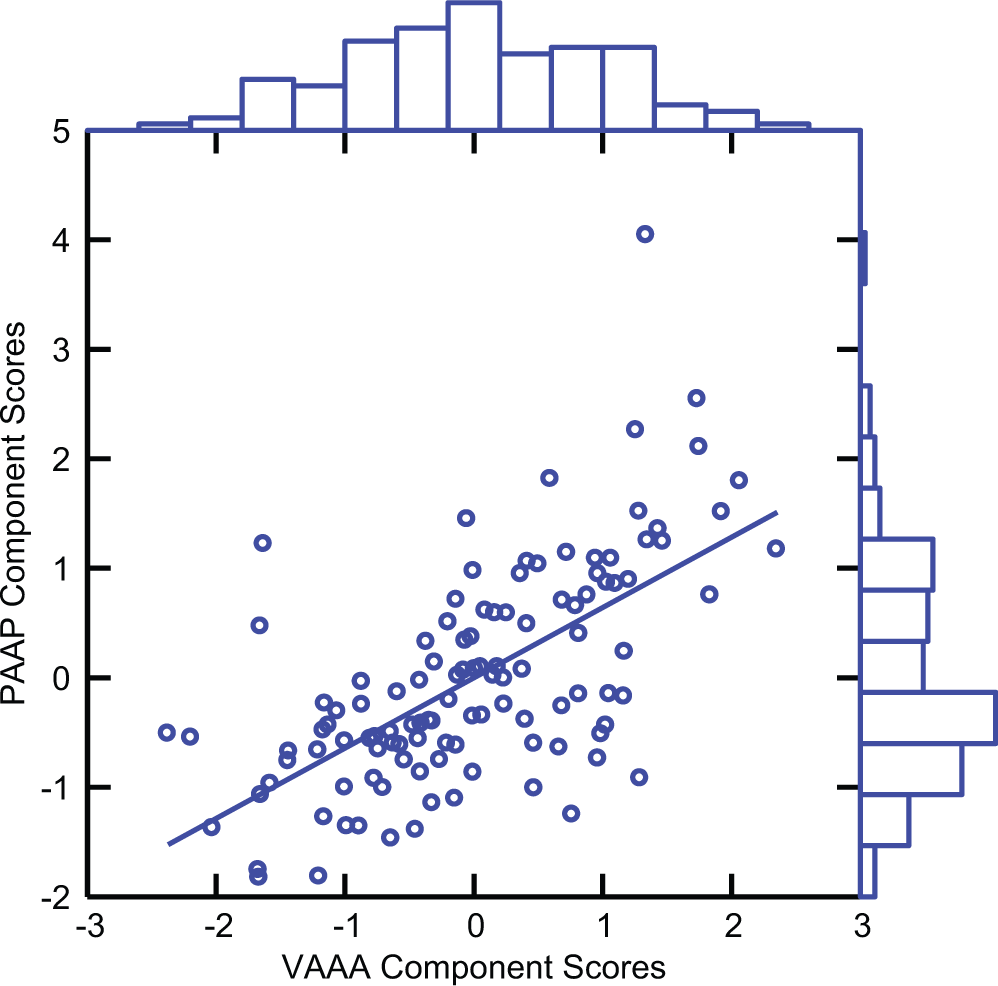
Distributions and scatterplot of component scores of Verbal Aggression Against Adults (VAAA) and Physical Aggression Against Peers (PAAP).

The univariate distributions in Figure 1 suggest that the distribution of the component scores of VAAA is closer to a normal distribution than the distribution of the component scores of PAAP. Table 1 quantifies this impression.

Table 1.

Descriptive Statistics of Component Scores of Verbal Aggression Against Adults (VAAA) and Physical Aggression Against Peers (PAAP).

	VAAA component scores	PAAP component scores
Number of cases	114	114
Minimum	−2.374	−1.829
Maximum	2.354	4.040
Arithmetic mean	0.000	0.000
Standard deviation	1.000	1.000
Skewness (G1)	−0.017	0.868
Standard error of skewness	0.226	0.226
Kurtosis (G2)	−0.476	1.450
Standard error of kurtosis	0.449	0.449
Shapiro–Wilk statistic	0.993	0.956
Shapiro–Wilk p value	0.816	0.001
Anderson–Darling statistic	0.223	1.213
Adjusted Anderson–Darling statistic	0.224	1.221
p Value	>.15	<.01

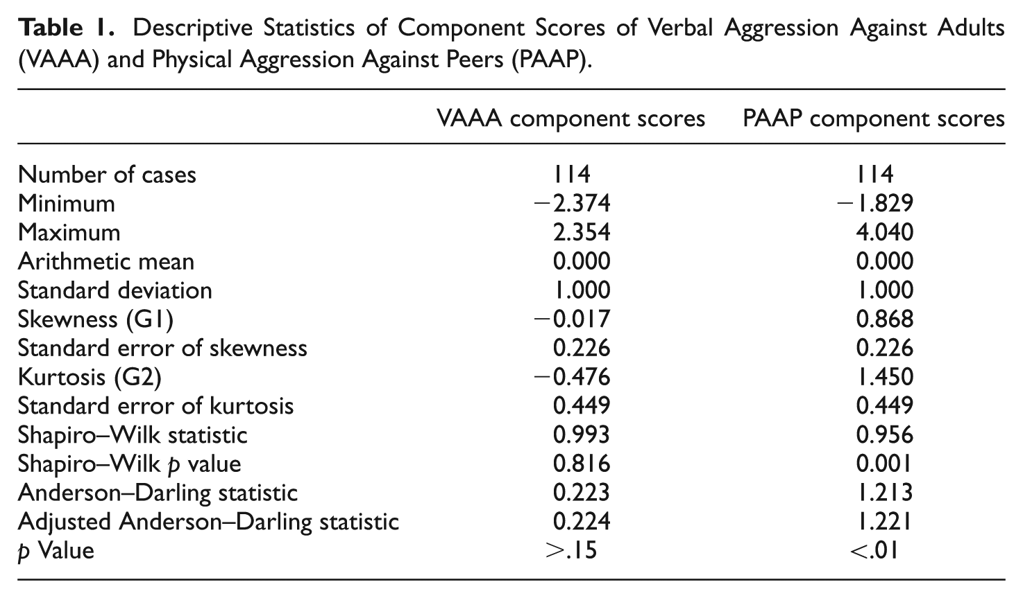
The results in Table 1 suggest that neither skewness nor kurtosis of the component scores of VAAA is excessive. In addition, neither the Shapiro–Wilk statistic nor the Anderson–Darling statistic suggests that the component scores of VAAA deviate significantly from normality. In contrast, all measures suggest that the component scores of PAAP are non-normally distributed.

The correlation between the two component score variables is r = 0.642. The ratio of the two skewness measures is, therefore, r³ = 0.265, suggesting that 26.5% of the skewness of the component scores of VAAA is left unexplained by the skewness of PAAP. The ratio of the two kurtosis measures is r⁴ = 0.170, suggesting that 17% of the kurtosis of the component scores of VAAA is left unexplained by the kurtosis of PAAP. Using the above decision rules, we, therefore, conclude that the direction of effect goes from PAAP to VAAA.

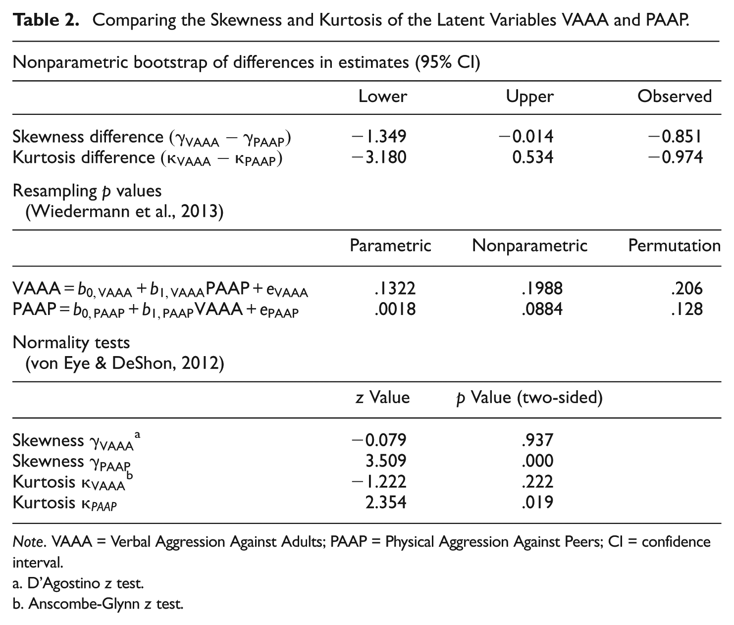
To support this conclusion, we compared the skewness and kurtosis of the latent variables VAAA and PAAP by using the three test procedures mentioned above, that is, the skewness and kurtosis tests proposed by D’Agostino (1971), Anscombe and Glynn (1983), a nonparametric bootstrap procedure based on the differences in skewness and kurtosis proposed by Pornprasertmanit and Little (2012), and the three resampling tests proposed by Wiedermann et al. (2013) to evaluate residuals of competing regression models. Table 2 displays the results of these tests.

Table 2.

Comparing the Skewness and Kurtosis of the Latent Variables VAAA and PAAP.

Nonparametric bootstrap of differences in estimates (95% CI)
	Lower	Upper	Observed
Skewness difference $(γ_{VAAA} - γ_{PAAP})$	−1.349	−0.014	−0.851
Kurtosis difference $(κ_{VAAA} - κ_{PAAP})$	−3.180	0.534	−0.974
Resampling p values (Wiedermann et al., 2013)
	Parametric	Nonparametric	Permutation
$VAAA = b_{0, VAAA} + b_{1, VAAA} PAAP + e_{VAAA}$	.1322	.1988	.206
$PAAP = b_{0, PAAP} + b_{1, PAAP} VAAA + e_{PAAP}$	.0018	.0884	.128
Normality tests (von Eye & DeShon, 2012)
	z Value	p Value (two-sided)
Skewness $γ_{VAAA}$ ^a	−0.079	.937
Skewness $γ_{PAAP}$	3.509	.000
Kurtosis $κ_{VAAA}$ ^b	−1.222	.222
Kurtosis $κ_{PAAP}$	2.354	.019

Note. VAAA = Verbal Aggression Against Adults; PAAP = Physical Aggression Against Peers; CI = confidence interval.

D’Agostino z test.

Anscombe-Glynn z test.

The test results shown in Table 2 can be interpreted as in support of the decision that VAAA is the outcome variable and PAAP is the explanatory variable. The only exception to this interpretation is the kurtosis difference κ_VAAA−κ_PAAP. This difference is nonsignificant. In all other cases, VAAA deviates less from normality than PAAP.

Latent Variable Scores in Structural Equation Models

In this section, we first review methods of estimation latent variable scores other than component scores. We discuss direction of effects in the context of structural modeling, and then apply the methods described in the last section in the context of latent variables analysis. For latent variable models other than PCA, a number of models have been discussed.

To describe the methods of estimation, we use the following notation (see Bartholomew & Knott, 1999; Jöreskog, Sörbom, & Yang-Wallentin, 2006; Lastowicka & Thamodaran, 1991).

X = n×p matrix of p standardized variables, observed on n cases, with (1/(n− 1))X′X = R, the correlation matrix of the p variables

F = an n×r matrix of standardized scores of r latent variables, for example, common factors, with r < p and (1/(n− 1))F′F = Φ, the correlation matrix of the r latent variables

S = an n×p matrix of standardized scores on p unique, independent latent variables (one such variable per observed variable) such that 1/(n− 1))S′S = I. These latent variables are independent of the latent variables in F, that is, (1/(n− 1))SF′ is a p×r null matrix

B = a p×r matrix of weights of the latent variables in F

U = a p×p diagonal matrix of weights of the latent variables in S

The model that we consider is

X = FB' + SU .

This model proposes that the p observed variables can be explained as a function of r+p latent variables. There is an extensive body of literature on the problem of indeterminacy of latent variable scores. This literature will not be reviewed here (see, e.g., Bartholomew & Knott, 1999; McDonald & Burr, 1967). Instead, we now present four of the better known methods of estimation of latent variable scores (Hershberger, 2005; Lastowicka & Thamodaran, 1991).

Least squares estimation (Horst, 1965). This method estimates F such that the trace Tr(Y S S′U) is minimized as

\hat{F_{t}} XB {(B' B)}^{- 1} .

Bartlett’s (1937) method takes into account the differences in the variances of the unique latent variables. The residuals are minimized weighted by the reciprocals of the standard deviations of the unique latent variables. The following estimates result:

\hat{F_{H}} = X U^{- 2} B {(B' U^{- 2} B)}^{- 1} .

Thurstone’s (1935) method assumes regression weights, M. Using these weights, latent variable scores can be estimated from the observed variables via

\hat{F_{m}} = XM' .

An OLS solution for M′ is R⁻¹ times the correlations between the observed and the latent variables. Because the correlations between the observed variables and the latent variable scores are BΦ, Thurstone’s factor scores can be estimated by

\hat{F_{m}} = X R^{- 1} B Φ .

Anderson and Rubin’s (1956) method represents an improvement over Bartlett’s (1937) method. Bartlett’s method yields correlated latent variable scores even when the latent variables are theoretically orthogonal. The matrix of correlations among Anderson–Rubin estimates is always an identity matrix. The estimates are

\hat{F_{AR}} = X U^{- 2} B {(B' U^{- 2} R U^{- 2} B)}^{1 / 2} .

The following are three desirable characteristics of latent variable scores (McDonald & Burr, 1967). First, latent variable scores should be highly correlated with their corresponding theoretical factors. This characteristic has been called the validity of latent variable scores. Second, when the latent variables are orthogonal, the scores from different latent variables should be uncorrelated also. In turn, when the latent variables are correlated, the correlations among scores from different latent variables should be close to the correlations among the corresponding latent variables. Estimates with these characteristics are called univocal. Third, the variances of the estimates should be the same as the variances of the corresponding latent variables.

For the following considerations, we opt for Anderson and Rubin’s (1956) method. The main reason for this is that we need to be in a situation in which lack of correlation translates in lack of directional dependency. Anderson and Rubin’s (1956) method is implemented in a number of software packages, for example in LISREL (Jöreskog et al., 2006).

The examination of directional dependence of latent variables in a structural model proceeds in a fashion parallel to the procedures used for manifest variables or principal components. Consider two latent variables, X and Y, on the y-side of a model that are not connected by way of a covariance or a path. That is, β_YX = β_XY = ψ_XY = 0. The skewness of the F_AR is

μ_{3} = \frac{E [{(F_{AR} - μ_{F_{AR}})}^{3}]}{σ_{F_{AR}}^{3}},

and the kurtosis of the F_AR is

μ_{4} = \frac{E [{(F_{AR} - μ_{F_{AR}})}^{4}]}{σ_{F_{AR}}^{4}} .

Now, let $κ_{F_{X}}$ be the coefficient of kurtosis of the Anderson–Rubin latent variable scores for X, and $κ_{F_{Y}}$ the coefficient of kurtosis for Y. Let $γ_{F_{X}}$ and $γ_{F_{Y}}$ be the corresponding skewness coefficients. Then, we can establish, in a fashion analogous to the one used for component scores, the two relationships $ρ^{3} = γ_{F_{Y}} / γ_{F_{X}}$ and $ρ^{4} = κ_{F_{Y}} / κ_{F_{X}} .$

Using these relationships, we derive conclusions about the direction of dependence between the latent variables X and Y. Specifically, if the direction of effect goes from X to Y, the following two predictions hold true:

$γ_{F_{Y}} < γ_{F_{X}}$

$κ_{F_{Y}} < κ_{F_{X}}$

Alternatively, decisions concerning the direction of effects can be made based on distributional properties of residuals of the two competing regression models $F_{Y} = b_{0, F_{Y}} + b_{1, F_{Y}} X + ϵ_{F_{Y}}$ and $F_{X} = b_{0, F_{X}} + b_{1, F_{X}} Y + ϵ_{F_{X}}$ . Again, $F_{Y}$ is classified as the response variable if $H_{0} : γ_{ϵ_{F_{X}}} = 0$ is rejected and $H_{0} : γ_{ϵ_{F_{Y}}} = 0$ is retained. If both null hypotheses are rejected/retained, the direction is uncertain (if it exists).

Data Example

For the following illustration, we use the same data as for the first example. Using the measures of Verbal Aggression Against Adults from 1983, 1985, and 1987 and the measures of Physical Aggression Against Peers, also from 1983, 1985, and 1987, we create a two-factor ML solution using LISREL 8.8 (the SIMPLIS command file for this model is reproduced in Appendix A). We label the two factors VAAA (for verbal aggression against adults) and PAAP (for physical aggression against peers).

We now proceed as follows. First, we calculate skewness and kurtosis of the factor scores of the two latent variables VAAA and PAAP, and then make a decision about direction of effect using the guidelines proposed above. The analyses of the factor scores were performed using SYSTAT 12. Second, we separately estimate the two competing regression models $F_{Y} = β_{0, F_{Y}} + β_{1, F_{Y}} X + ϵ_{F_{Y}}$ and $F_{X} = β_{0, F_{X}} + β_{1, F_{X}} Y + ϵ_{F_{X}}$ and evaluate distributional properties of model residuals to arrive at a decision concerning directional dependence. Note that this part of the analysis constitutes a two-step procedure, in which $F_{X}$ and $F_{Y}$ are first estimated in a structural model and then further analyzed using ordinary linear regression models. Third, we estimate a recursive latent variable model, in which we regress a common factor of PAAP onto a common factor of VAAA, and vice versa, to illustrate potential limitations in applying structural models for conclusions concerning the direction of effects.

The scatterplot of the factor scores for the VAAA and the PAAP factors are depicted in Figure 2. The univariate distributions appear on the margins of the plot.

Figure 2.

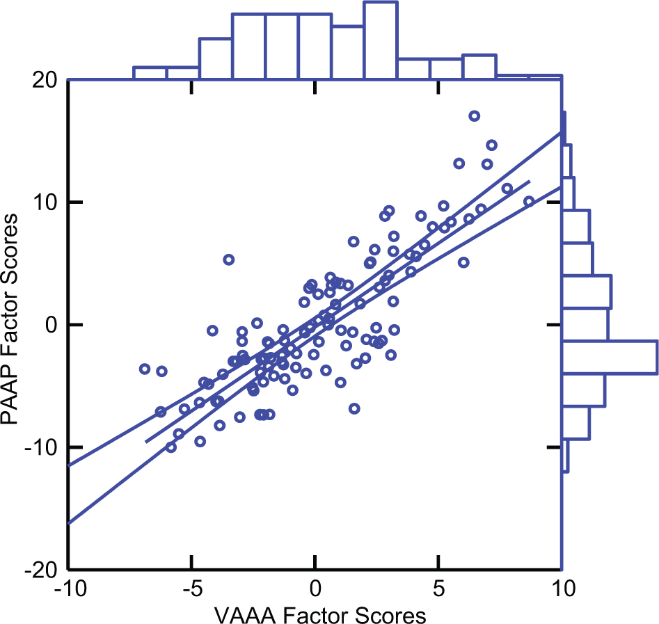
Distributions and scatterplot of factor scores of Verbal Aggression Against Adults (VAAA) and Physical Aggression Against Peers (PAAP).

The univariate distributions in the margins of Figure 2 suggest the same interpretation as the distributions in Figure 1. The distribution of the factor scores of VAAA is closer to a normal distribution than the distribution of the factor scores of PAAP. Table 3 quantifies this impression.

Table 3.

Descriptive Statistics of the Factor Scores of Verbal Aggression Against Adults (VAAA) and Physical Aggression Against Peers (PAAP).

	VAAA factor scores	PAAP factor scores
Number of cases	114	114
Minimum	−6.856	−10.072
Maximum	8.713	16.960
Arithmetic mean	0.320	0.228
Standard deviation	3.410	5.637
Skewness (G1)	0.206	0.628
Standard error of skewness	0.226	0.226
Kurtosis (G2)	−0.447	−0.035
Standard error of kurtosis	0.449	0.449
Shapiro–Wilk statistic	0.990	0.964
Shapiro–Wilk p value	0.531	0.004
Anderson–Darling statistic	0.262	1.370
Adjusted Anderson–Darling statistic	0.264	1.380
p Value	>.15	<.01

The results in Table 3 show a similar picture as the ones in Table 1. The factors scores of VAAA deviate from normality only randomly. In contrast, with the exception of the kurtosis measure, all measures suggest that the factor scores of PAAP are non-normally distributed.

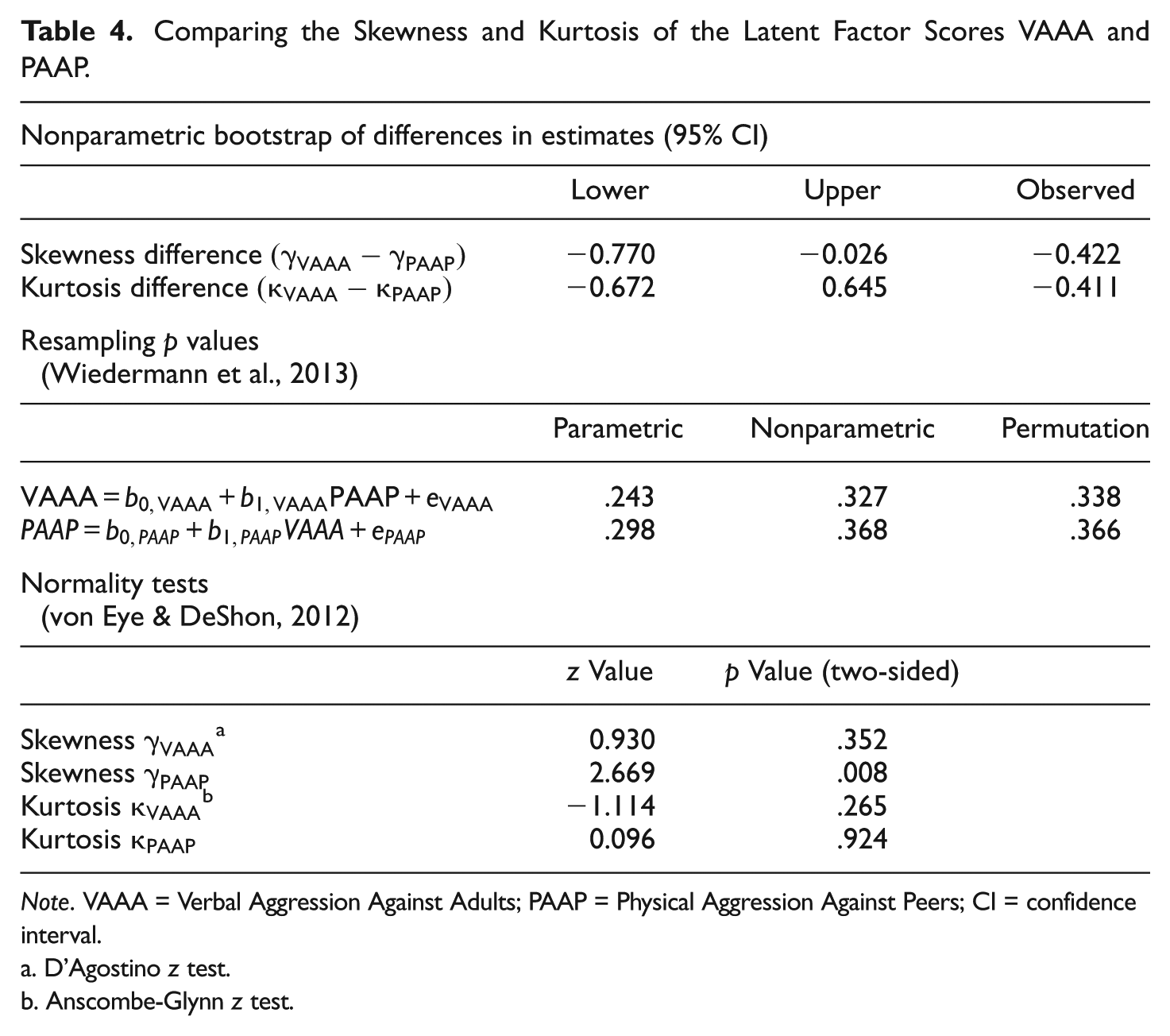
The correlation between the two-factor score variables is r = 0.828. The ratio of the two skewness measures is, therefore, r³ = 0.568, suggesting that 56.8% of the skewness of the factor scores of VAAA is explained by the skewness of the factor scores of PAAP. The ratio of the two kurtosis measures is r⁴ = 0.470, suggesting that 47% of the kurtosis of the factor scores of VAAA is explained by the kurtosis of the factor scores of PAAP. Using the above decision rules, we, therefore, conclude, on a descriptive level, that the direction of effect goes from Physical Aggression Against Peers to Verbal Aggression Against Adults. Table 4 shows the results for the nonparametric boostrapping procedure based on the differences of skewness and kurtosis estimates, the resampling p values obtained from the tests based on the skewness of the competing regression residuals, and the test statistics of D’Agostino’s test and the Anscombe–Glynn procedures. The bootstrapping confidence intervals suggest that skewness differences significantly differ from zero; however, there is no significant difference in kurtosis values. Furthermore, although resampling p values for the model $VAAA = b_{0, VAAA} + b_{1, VAAA} PAAP + e_{VAAA}$ are constantly smaller than those for the competing regression model, no decision concerning the response and the explanatory variable can be made. Finally, the normality tests suggest that the skewness of PAAP significantly deviates from zero, all remaining null hypotheses are retained and, thus, confirm the assumption of normality. Overall, there is only weak evidence that Verbal Aggression Against Adults is the response variable and Physical Aggression Against Peers is the explanatory variable.

Table 4.

Comparing the Skewness and Kurtosis of the Latent Factor Scores VAAA and PAAP.

Nonparametric bootstrap of differences in estimates (95% CI)
	Lower	Upper	Observed
Skewness difference $(γ_{VAAA} - γ_{PAAP})$	−0.770	−0.026	−0.422
Kurtosis difference $(κ_{VAAA} - κ_{PAAP})$	−0.672	0.645	−0.411
Resampling p values (Wiedermann et al., 2013)
	Parametric	Nonparametric	Permutation
$VAAA = b_{0, VAAA} + b_{1, VAAA} PAAP + e_{VAAA}$	.243	.327	.338
$PAAP = b_{0, PAAP} + b_{1, PAAP} VAAA + e_{PAAP}$	.298	.368	.366
Normality tests (von Eye & DeShon, 2012)
	z Value	p Value (two-sided)
Skewness $γ_{VAAA}$ ^a	0.930	.352
Skewness $γ_{PAAP}$	2.669	.008
Kurtosis $κ_{VAAA}$ ^b	−1.114	.265
Kurtosis $κ_{PAAP}$	0.096	.924

Note. VAAA = Verbal Aggression Against Adults; PAAP = Physical Aggression Against Peers; CI = confidence interval.

D’Agostino z test.

Anscombe-Glynn z test.

In the third analytic step, we regress latent variables of PAAP and VAAA onto each other within a structural model. In a first model, we posit that

The three measures of Physical Aggression against Peers are indicators of a latent variable, PAAP; this latent variable represents the time-invariant element of Physical Aggression against Peers

The three measures of Verbal Aggression against Adults are indicators of a latent variable, VAAA; this latent variable represents the time-invariant element of Verbal Aggression against Adults

PAAP is predictive of VAAA

This model converged, but failed to describe the data well (root mean square error of approximation = .17). Therefore, we introduced a developmental element and allowed the residuals of the first and third measures of PAAP and VAAA, that is, PAAP83 and VAAA83, as well as PAAP87 and VAAA87, to covary. Appendix B displays the LISREL command file for this model. The fit of this model was satisfactory (χ² = 10.83, df = 6, p = .09; root mean square error of approximation = .08 [.0; .16]; comparative fit index = .98; goodness of fit index = .97). In addition, all estimated loadings were significant, and so was the path from PAAP to VAAA (β₂₁ = 0.77, SE = 0.15, z = 5.27, p < .01). Figure 3 displays model and estimates (standardized scores given).

Figure 3.

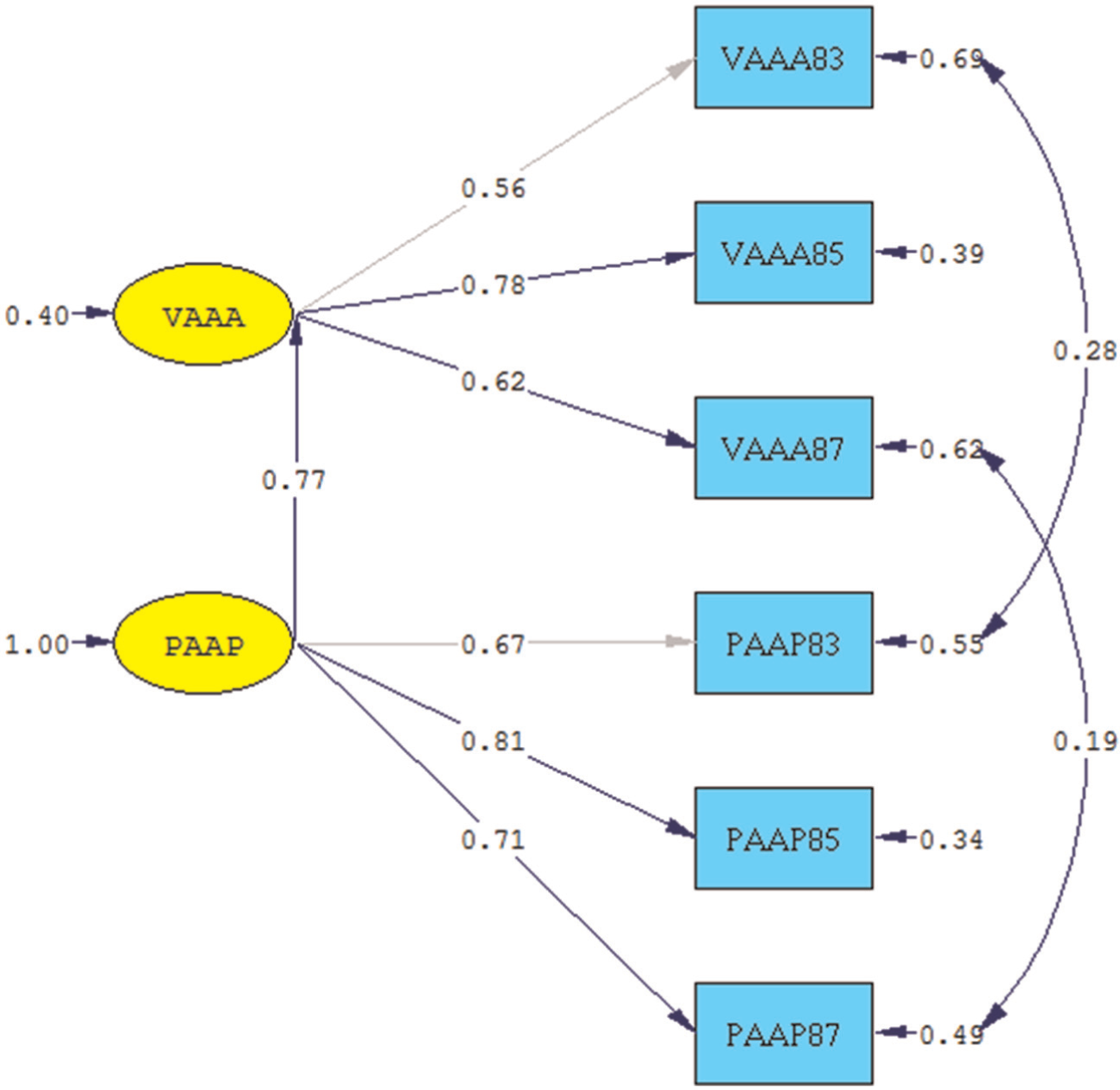
Predicting Verbal Aggression Against Adults (VAAA) from Physical Aggression Against Peers (PAAP).

We now reverse the path in this model so that PAAP is predicted from VAAA. All estimates and model fit (not shown here) are exactly the same. We conclude that structural models as estimated here cannot be used to make decisions about direction of dependence. Only when hypotheses about direction of dependence exist a priori, and when the reverse direction is illogical or implausible, results from models as the ones estimated here can be used to support or reject these hypotheses.

It is interesting to note that causal inferences are often drawn based on matrix B (Sobel, 1995). Specifically, under regularity conditions on B, the parameter π_rs of the reduced form equation

Y_{i} = α' + Π X_{i} + v_{i}

is usually interpreted as a standard regression parameter: the effect of a one-unit change in X_ir, that is, the rth element of X_i, on Y_is, that is, the sth element of Y_s. In Equation (43), $v_{i} = {(I - B)}^{- 1} ϵ_{i}$ , $α^{'} = {(I - B)}^{- 1} α$ , $Π = {(I - B)}^{- 1} Γ$ , and $Ψ = V (v_{i}) = {(I - B)}^{- 1} Σ {(I - B)}^{- 1}$ , for all i (Sobel, 1995). In econometric models, π_rs is called equilibrium multiplier. In psychology and sociology, π_rs is called total effect.

Similarly, the stability of a model is a sufficient condition for convergence. It is also estimated based on B. Specifically, it is defined as the largest eigenvalue of B′B which must be less than one for convergence. With respect to our discussion of direction dependence, we note that models of the form estimated in the present data example do not allow one to distinguish between direction of effect based on model stability. The models estimated for both direction of effect hypotheses come with largest eigenvalues of B′B of 0.597. We conclude that even when competing models converge properly and fit, conclusions concerning direction of effect require theory and the methods discussed in this article.

Discussion

The application of methods for the determination of directional dependence is most important in the context of observational research. In this context, manipulation of independent variables, randomization of potential confounders, repetition of observation, or unbiased selection of participants are often impossible. Still, researchers entertain hypotheses about directional dependence even when data are collected in observational studies and in natural settings. Here, the methods discussed in this article are most useful.

However, it can be risqué to base decisions about direction of effects solely on the results of the procedures proposed here.

Therefore, researchers can do worse than considering guidelines such as the ones proposed by Hill (1965; cf. Cox & Wermuth, 2001; Lynd-Stevenson, 2007). According to these guidelines, a dependency is more likely to be causal if

Researchers have developed an a priori explanation of the processes under study.

Researchers have derived such an explanation based on the results of a study. Here, the methods proposed in this article can play an important role. It should be noted, however, that a priori explanations typically carry more weight than ex post explanations.

The studied effect is large; the reason for this part of the guidelines is that, if an effect is large, it becomes less likely that alternative explanations surface by way of unmeasured confounding variables.

If the hypothesized dependency is characterized by a process that involves the same type of relationship as involved in the statistical analysis. In the current context, relationships are examined in the context of a linear, regression-type model. Therefore, conclusions drawn from applications of the methods presented in this article are more convincing if researchers can make plausible that the processes under study can validly be depicted using linear models.

If the same effect, that is, the same conclusion about directional dependence is also found in independent studies which, preferably, are of different design and involve different methods of data collection (see also Lynd-Stevenson, 2007).

If variable relationships can be considered internally and externally valid.

If the dependence is the result of an intervention. This last element of the guideline may be of lesser importance in observational studies. Intervention in natural settings cannot always be performed as cleanly as a lab experiment (Spiel et al., 2008).

If these conditions are fulfilled, dependence can be considered more likely to be causal. The methods developed here add a statistical tool to the decision process. Dependence can be considered directed, which is one of the bases of causal dependence, if the skewness scores and the kurtosis scores of the latent putative explanatory and outcome variables are related as discussed in this article.

The present study focused on the theoretical underpinnings of direction of dependence methods in the context of latent variable modeling and illustrated an application of this methodology using two empirical examples. It is up to future studies to evaluate the Type I error robustness and power behavior of the discussed tests under various scenarios using intensive Monte Carlo simulation experiments.

Footnotes

Appendix A

Appendix B

Acknowledgements

The authors are indebted to J. J. McArdle and Ingo Nader for encouraging and helpful comments on earlier drafts of this article.

Declaration of Conflicting Interests

The author(s) declared no potential conflicts of interest with respect to the research, authorship, and/or publication of this article.

Funding

The author(s) received no financial support for the research, authorship, and/or publication of this article.

References

Anderson

T. W.

Rubin

(1956). Statistical inference in factor analysis. In Proceedings of the Third Berkeley Symposium on Mathematical Statistics and Probability (pp. 111-150). Berkeley: University of California Press.

Anscombe

F. J.

Glynn

W. J.

(1983). Distribution for the kurtosis statistic b2 for normal samples. Biometrika, 70, 227-234.

Bartholomew

D. J.

Knott

(1999). Latent variable models and factor analysis. London, England: Arnold.

Bartlett

M. S.

(1937). The statistical conception of mental factors. British Journal of Psychology, 28, 97-104.

Bentler

P. M.

(1983). Some contributions to efficient statistics in structural models: Specification and estimation of moment structures. Psychometrika, 48, 493-517.

Browne

M. W.

(1982). Covariance structures. In Hawkins

D. M.

(Ed.), Topics in applied multivariate analysis (pp. 72-141). Cambridge, England: Cambridge University Press.

Browne

M. W.

(1984). Asymptotically distribution-free methods for the analysis of covariance structures. British Journal of Mathematical and Statistical Psychology, 9, 665-672.

Cox

D. R.

Wermuth

(2001). Some statistical aspects of causality. European Sociological Review, 17, 65-74.

D’Agostino

R. B.

(1971). Transformation to normality of the null distribution ofg₁. Biometrika, 57, 341-348.

10.

D’Agostino

R. B.

Belanger

D’Agostino

R. B.

Jr. (1990). A suggestion for using powerful and informative tests of normality. American Statistician, 44, 316-321.

11.

D’Agostino

R. B.

Pearson

E. S.

(1973). Testing departures from normality. 1. Fuller empirical results for the distribution of b₂ and √b₁. Biometrika, 60, 613-622.

12.

Dodge

Rousson

(2000). Direction dependence in a regression line. Communications in Statistics—Theory and Methods, 32, 2053-2057.

13.

Dodge

Rousson

(2001). On asymmetric properties of the correlation coefficient in the regression setting. American Statistician, 55, 51-54.

14.

Dodge

Yadegari

(2010). On direction of dependence. Metrika, 72, 139-150.

15.

Finkelstein

J. W.

von Eye

Preece

M. A.

(1994). The relationship between aggressive behavior and puberty in normal adolescents: A longitudinal study. Journal of Adolescent Health, 15, 319-326.

16.

Hershberger

S. L.

(2005). Factor score estimation. In Everitt

B. S.

Howell

D. C.

(Eds.), Handbook of statistics in social science (pp. 636-644). Chichester, England: Wiley.

17.

Hill

A. B.

(1965). The environment and disease: Association or causation. Proceedings of the Royal Society of Medicine, 58, 295-300.

18.

Hogg

R. V.

Tanis

E. A.

(1993). Probability and statistical inference (4th ed.). New York, NY: MacMillan.

19.

Horst

(1965). Factor analysis of data matrices. New York, NY: Holt, Rinehart, & Winston.

20.

Jöreskog

K. G.

Sörbom

Yang-Wallentin

(2006). Latent variable scores and observational residuals. Retrieved from http://www.ssicentral.com/lisrel/techdocs/obsres.pdf

21.

Jöreskog

Yang

(1996). Non-linear structural equation models: The Kenny-Judd model with interaction effects. In Marcoulides

Schumacker

(Eds.), Advanced structural equation modeling: Concepts, issues, and applications (pp. 57-87). Thousand Oaks, CA: Sage.

22.

Kim

J. M.

(2013). Analysis of directional dependence using asymmetric copula-based regression models. Journal of Statistical Computation and Simulation. Advance online publication. doi:10.1080/00949655.2013.779696

23.

Lastowicka

J. L.

Thamodaran

(1991). Common factor score estimates in multiple regression problems. Journal of Marketing Research, 28, 105-112.

24.

Lynd-Stevenson

R. M.

(2007). Concerns regarding the traditional paradigm for causal research: The unified paradigm and causal research in scientific psychology. Review of General Psychology, 11, 286-304.

25.

Mardia

K. V.

(1970). Measures of multivariate skewness and kurtosis with applications. Biometrika, 57, 519-530.

26.

Mardia

K. V.

(1980). Tests of univariate and mutivariate normality. In Krishnaiah

P. R.

(Ed.), Handbook of statistics (Vol. 1, pp. 279-320). Amsterdam, Netherlands: North Holland.

27.

McDonald

R. P.

Burr

E. J.

(1967). A comparison of four methods of constructing factor scores. Psychometrika, 32, 381-401.

28.

Micceri

(1989). The unicorn, the normal curve, and other improbable creatures. Psychological Bulletin, 105, 156-166.

29.

Muddapur

M. V.

(2003). On directional dependence in a regression line. Communications in Statistics—Theory and Methods, 32, 2053-2057.

30.

Nigg

J. T

Knottnerus

G. M.

Martel

M. M.

Nikolas

Cavanagh

Karmaus

Rappley

M. D.

(2008). Low blood lead levels associated with clinically diagnosed attention-deficit/hyperactivity disorder and mediated by weak cognitive control. Biological Psychiatry, 63, 325-331.

31.

Pearl

(2012). The causal foundations of structural equation modeling. In Hoyle

R. H.

(Ed.), Handbook of structural equation modeling (pp. 68-91). New York, NY: Guilford.

32.

Pearson

(1895). Contributions to the mathematical theory of evolution, II: Skew variation in homogeneous material. Philosophical Transactions of the Royal Society of London, 186, 343-414.

33.

Pornprasertmanit

Little

T. D.

(2012). Determining directional dependency in causal associations. International Journal of Behavioral Development, 36, 313-322.

34.

Shimizu

Hoyer

P. O.

Hyvärinen

Kerminen

(2006). A linear non-Gaussian acyclic model for causal discovery. Journal of Machine Learning Research, 7, 2003-2030.

35.

Shimizu

Kano

(2008). Use of non-normality in structural equation modeling: Application to direction of causation. Journal of Statistical Planning and Inference, 138, 3483-3491.

36.

Sobel

(1995). Causal inference in the social and behavioral sciences. In Arminger

Clogg

C. C.

Sobel

(Eds.), Handbook of statistical modeling for the social and behavioral sciences (pp. 1-38). New York, NY: Plenum.

37.

Sobel

(1996). An introduction to causal inference. Sociological Methods & Research, 24, 353-379.

38.

Spiel

Gradinger

Lapka

Zodlhofer

E. M.

Reimann

Schober

Wagner

von Eye

(2008). An Euclidean distance score matching procedure for nonexperimental comparison studies. European Psychologist, 13, 180-187.

39.

Steinley

McDonald

R. P.

(2007). Examining factor score distributions to determine the nature of latent spaces. Multivariate Behavioral Statistics, 42, 133-156.

40.

Sungur

E. A.

(2005). A note on directional dependence in regression setting. Communications in Statistics—Theory and Methods, 34, 1957-1965.

41.

Thurstone

L. L.

(1935). Vectors of the mind. Chicago, IL: University of Chicago Press.

42.

von Eye

DeShon

R. P.

(2008). Characteristics of measures of directional dependence—A Monte Carlo study. InterStat. Retrieved from http://interstat.statjournals.net/YEAR/2008/articles/0802002.pdf

43.

von Eye

DeShon

R. P.

(2012). Directional dependency in developmental research. International Journal of Behavior Development, 36, 303-312.

44.

von Eye

Gardiner

J. C.

(2004). Locating deviations from multivariate normality. Understanding Statistics, 3, 313-331.

45.

Walwyn

(2005). Moments. In Everitt

B. S.

Howell

D. C.

(Eds.), Handbook of statistics in social science (pp. 1258-1260). Chichester, England: Wiley.

46.

Wiedermann

Hagmann

Kossmeier

von Eye

(2013). Resampling techniques to determine direction of effects in linear regression models. InterStat. Retrieved from http://interstat.statjournals.net/YEAR/2013/articles/1305002.pdf