A Comprehensive Approach for Assessing Person Fit With Test

Abstract

Item response theory (IRT) models allow model–data fit to be assessed at the individual level by using person-fit indices. This assessment is also feasible when IRT is used to model test–retest data. However, person-fit developments for this type of modeling are virtually nonexistent. This article proposes a general person-fit approach for test–retest data, which is based on practical likelihood-based indices. The approach is intended for two types of assumption regarding trait levels—stability and change—and can be used with a variety of IRT models. It consists of two groups of indices: (a) overall indices based on the full test–retest pattern, which are more powerful and are intended to flag a respondent as potentially inconsistent; and (b) partial indices intended to provide additional information about the location and sources of misfit. Furthermore, because the overall procedures assume local independence under repetition, a statistic for assessing the presence of retest effects at the individual level is also proposed. The functioning of the procedures was assessed by using simulation and is illustrated with two empirical studies: a stability study based on graded-response items and a change study based on binary items. Finally, limitations and further lines of research are discussed.

Keywords

person-fit test–retest data stability designs measurement of change retest effects

Person-fit indices based on a parametric item response theory (IRT) model aim to trace test response patterns that are inconsistent given (a) the item parameter values and (b) the trait estimate of the respondent (e.g., Meijer & Sijtsma, 2001). In particular, practical or nonspecific indices (Drasgow, Levine, & McLaughlin, 1987, 1991; Ferrando, in press) assess the null hypothesis that the pattern is consistent against no specific alternative (i.e., specific type of misfit), and they can therefore be regarded as the simplest and least informative model-based person-fit indices (Drasgow et al., 1987). In spite of this limitation, however, practical indices are quite useful as broad-screening tools for flagging potentially problematic patterns. Once a pattern has been detected, further information must be obtained so that the practitioner can decide what to do with the pattern in each case (e.g., Smith, 1986).

Of the considerable number of existing nonspecific indices (e.g., Meijer & Sijtsma, 2001), this article focuses on the likelihood-based (L-B) indices initially proposed by Levine and Rubin (1979). Basic L-B indices (which are reviewed below) have a clear rationale, are easy to compute, and generally perform as well as or better than the alternatives (Li & Olejnik, 1997; Nering & Meijer, 1998; Reise & Due, 1991).

In spite of these strengths, L-B indices also have a series of practical shortcomings, the most important of which is their low detection power. The most basic factor that can determine power is test length (see, e.g., Reise & Due, 1991) or, more specifically, the number of item scores used to compute the index. Now, in most applications, this number is simply too small to permit efficient and powerful detection of misfit (Drasgow et al., 1991; Ferrando, in press).

So far, the main improvement in terms of increasing power has been the development of person-fit procedures intended for multidimensional or multiscale tests (Drasgow et al., 1991; Ferrando, in press). The multidimensional proposals potentially have two main advantages. First, they provide additional information (which is obtained from the various subscales) about the sources of inconsistency. Second, they make it possible to compute multiscale L-B indices that are based on a larger number of item scores that are, therefore, more powerful.

The present article discusses the improvements that can be made to L-B indices when there is a different source of additional information: that which can be obtained when a given instrument is administered on two occasions to the same individuals (i.e., a test–retest design). This type of general design is commonly used to assess reliability (Morrison, 1981). Furthermore, in clinical settings, test–retest designs are commonly used to assess trait changes due to the effects of treatments (Reise & Haviland, 2005). Also, in the selection domain, they are used to gauge the effects of test coaching and practice (e.g., Hausknecht, Trevor, & Farr, 2002). In all these scenarios, assessing individual consistency is very important. As discussed below, a test–retest design might provide more accurate trait estimates or individual estimates of change. However, the individual estimates of interest can only be validly interpreted if the responses that the individual gives at Time 1 and Time 2 are consistent.

In spite of the widespread use of test–retest designs and the importance of assessing individual consistency when they are used, person-fit proposals based on test–retest data are very scarce. As far as the writer knows, only Ferrando (2010) has proposed a binary response-specific procedure based on the responses that change between the first and the second administrations.

The main purpose of this article is to develop and propose a series of L-B procedures for assessing person fit based on test–retest data. The general proposal is thought to be comprehensive for two main reasons. First, the L-B extensions and improvements can be used with both binary and graded response items, so they can be based on a variety of IRT models. Second, procedures are developed for both stability and change conditions. Overall, the procedures proposed here are expected to cover most of the test–retest assessments that are made in practical applications.

The rest of the article is organized as follows. First, the basic L-B indices intended for a single test administration are reviewed so as to provide a basis for the present developments. Second, the procedures proposed here are presented, and the practical conditions in which they are expected to work appropriately are discussed. Third, the problem of potential retest effects is considered, and a new index for assessing these effects at the individual level is proposed. Finally, the functioning of the proposed procedures is assessed by means of a simulation study and illustrated with two empirical studies.

Review of the Basic L-B Indices

As discussed above, two types of item response formats will be considered: binary (scored as 0, 1) and graded (scored with successive integers). In both cases, it will be assumed that the j = 1, 2, . . ., n test items are well fitted by a unidimensional IRT model and that the item parameter estimates are fixed (see, e.g., Zimowski, Muraki, Mislevy, & Bock, 2003) so that, in the scoring stage, maximum likelihood (ML) individual trait estimates are obtained based on the fixed item parameters. These assumptions are very general and can be used in a wide range of IRT models. For the moment, however, the article will focus on only two models: the two-parameter logistic model (2PM) for binary responses and Samejima’s (1969) graded response model (GRM). Space constraints do not allow a more detailed technical discussion of the models and estimation procedures, and the interested reader is referred to Baker and Kim (2004) and Zimowski et al. (2003) for further information.

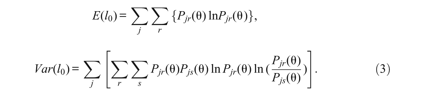
The basic rationale on which L-B indices are based is that the likelihood function value of a particular response pattern will be large for patterns that are consistent with the model and small for patterns that are not (Levine & Rubin, 1979). Under the conditions discussed above (fixed and known item parameters), the log-likelihood index l ₀ is simply the logarithm of the likelihood function evaluated at the maximizing value of θ (i.e., the ML trait-level estimate). The expression for l ₀ that follows is general and applies to both binary and graded-response models.

l_{0} ({\hat{θ}}_{i}) = \sum_{j} \sum_{r} u_{i j r} ln P_{j r} ({\hat{θ}}_{i}),

where ${\hat{θ}}_{i}$ is the ML trait estimate of individual i, u_ijr = 1 if respondent i chooses category r for item j, and u_ijr = 0 otherwise, and P_jr is the model-based probability of scoring r on item j given the item parameters and the trait estimate of the individual.

Type (1) indices have three important shortcomings. First, they depend on test length. Second, they are not independent of trait level. And finally, they lack reference values. To make up for these drawbacks, Drasgow, Levine, and Williams (1985) derived the standardized version:

l_{Z} = \frac{l_{0} - E (l_{0})}{\sqrt{V a r (l_{0})}},

where the mean and variance are given by

\begin{array}{l} E (l_{0}) = \sum_{j} \sum_{r} {P_{j r} (θ) ln P_{j r} (θ)}, \\ V a r (l_{0}) = \sum_{j} [\sum_{r} \sum_{s} P_{j r} (θ) P_{j s} (θ) ln P_{j r} (θ) ln (\frac{P_{j r} (θ)}{P_{j s} (θ)})] . \end{array}

If the “true”θ trait levels are known and used in Equations (3), and the test is long enough, then the standardized indices in (2) are expected to follow a standard normal distribution under the null hypothesis of consistency (Drasgow et al., 1985). In practice, however, θ is unknown and the ML estimate is used in its place. Research suggests that (a) the use of a trait estimate instead of the true level generally leads to a negatively skewed distribution of the statistic, the variance of which is smaller than the expected unit value, and (b) the shorter the test is, the worse the problem becomes (Nering, 1995; Reise, 1995). The departure from the reference distribution in real applications is indeed an important problem and continues to receive attention in the literature (Seo & Weiss, 2013). However, as discussed below, strict adherence to the theoretical distribution is more important when the index is intended to be used as a rigorous detection device than when it is intended to be used as a first-step screening device (the aim of this article). So, in principle, the l_z values considered here will be interpreted as (approximately) standard normal z scores.

At the conceptual level, l_z mainly measures a type of misfit that can be referred to as “violation to a Guttman pattern” (Meijer, 2003). Thus, in the binary case, which is the clearest, a well-fitting, scalable pattern is one in which the respondent tends to endorse the items whose difficulty index is below his/her estimated trait level but not endorse the items whose difficulty index is above it. Nonfitting patterns are those in which the pattern of endorsement is not consistent with the ordering of items by their difficulty. As for interpretation, a large negative value relative to the standard normal distribution is an indicator that the pattern is inconsistent with the model and the estimated trait value. A large positive value indicates that the pattern is more deterministic or scalable than the stochastic model predicts.

Proposed Approach and Rationale

Assume now that the test with n items is administered to the same respondents at two points in time with a given retest interval and denoted by a prime the responses given at Time 2. L-B-based retest procedures will now be proposed for two types of situation: stability and change. In the first situation, the trait level of the respondent is assumed to be the same at both points in time. In the second, the trait levels are assumed to be different. The position taken here is that, when possible, these basic assumptions should be guided by the specific design that is used, and in this respect, two types of basic design are considered. In the first type, (a) a stable trait is measured, (b) the retest interval is not long enough to give rise to trait changes, and (c) no treatment is given during the retest interval, and the conditions of administration are the same at both points in time (see Goldberg, 1963). These conditions make it reasonable to assume trait stability. On the other hand, designs of the second type are generally pretest–treatment–posttest designs (Shadish, Cook, & Campbell, 2002) for assessing individual changes in the trait level due to the effects of the treatment. When they are used, the trait levels of the respondent are expected to be different at Time 1 and Time 2. In practice, the first type of design is usually applied in test–retest reliability studies (Goldberg, 1963; Morrison, 1981). For their part, change designs are widely used in the clinical and organizational settings discussed above.

In some applications, it is certainly true that the design-guided stability versus change distinction is not so clear, so the choice of the appropriate procedure is more data specific. One example would be an exploratory study that aims to assess whether an increased retest interval leads to trait changes or not. Finally, more complex designs may require both procedures to be combined. As an example, consider a two-group retest design in which the stability procedure is appropriate for the control group whereas the change procedure is appropriate for the experimental group.

In both types of procedure, the developments proposed here are based on two additional assumptions. First, the item parameters (which are taken as fixed) are assumed to be the same at Time 1 and Time 2. Second, the local independence principle is also assumed to hold for repeated measurements of the same item or, more specifically, for fixed θ_i the conditional distributions of the responses to the same item in two repeated administrations are independent of each other. The plausibility of these assumptions is further discussed below.

Proposed Procedures When Trait Stability Is Assumed

Because θ_i is assumed to be the same at both points in time, it is proposed to obtain a common ML trait estimate by treating the test–retest pattern as if it were a single response pattern made up of 2n responses. So, in accordance to the developments in the section above, and the two assumptions stated, the log-likelihood retest index in this case (l₀-rts) is given by

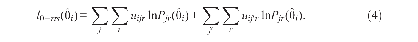
l_{0 - r t s} ({\hat{θ}}_{i}) = \sum_{j} \sum_{r} u_{i j r} ln P_{j r} ({\hat{θ}}_{i}) + \sum_{j'} \sum_{r} u_{i j' r} ln P_{j r} ({\hat{θ}}_{i}) .

Note that no prime in (4) is used to distinguish the trait estimate in either of the sum terms because this estimate is common. Neither is a prime used in the P_jr terms because they are also the same given the assumption of invariant item parameters. It follows that the mean and variance of l₀-rts are (see Equation 3)

E (l_{0 - r t s} ({\hat{θ}}_{i})) = 2 E (l_{0} ({\hat{θ}}_{i})); V a r (l_{0 - r t s} ({\hat{θ}}_{i})) = 2 V a r (l_{0} ({\hat{θ}}_{i})) .

So, the standardized index that is proposed in this case is

l_{z - r t s} = \frac{l_{0 - r t s} - E (l_{0 - r t s})}{\sqrt{V a r (l_{0} - r t s)}} .

As in the case of l_z based on a single test administration, the reference distribution for l_z-rts is the standard normal. However, the retest version is expected to be closer to the reference distribution for two reasons. First, the ML trait estimate is obtained from a response pattern that is twice as long. So, it is expected to be more accurate and closer to the “true” trait level (provided indeed that the responses are consistent). Second, the L-B index is obtained from a sum of 2n locally independent terms instead of the n terms in the single index. So, by asymptotic theory, its distribution is expected to better approach the normal. Regarding person-fit functioning, because the number of item scores from which the index is computed is now twice as long, l_z-rts is expected to be more powerful than the corresponding index based on a single administration.

Smith (1986) proposed a residual statistic based on the Rasch model for assessing the constancy of the trait estimate across different parts of the test. In Smith’s proposal (a) a common trait estimate was obtained from the entire pattern, (b) the pattern was split up into a number of parts, and (c) it was checked whether the common trait estimate was able to account for all partial response patterns. Now, it is clear that the present proposal is quite close to Smith’s rationale if the Time 1 and Time 2 response patterns are viewed as partial splits of the 2n response pattern. Continuing with Smith’s rationale, further information can be gained if, in addition to the total l_z-rts statistic, the standard l_z statistic in (2) is also computed separately in the Time 1 and Time 2 response patterns but using the common trait estimate in both cases. For example, suppose that a respondent answers consistently at Time 1 but loses interest during the second administration and answers almost randomly at Time 2. The total l_z-rts is expected to detect that, overall, the responses of this individual are inconsistent. If it does, the additional separate analyses would reveal consistency at Time 1 but inconsistency at Time 2.

Proposed Procedures When Change Is Assumed

The trait level of the individual is now assumed to be different at Time 1 (θ_i) and Time 2 (θ′_i), and the issue of most interest is, generally, the assessment of individual change.

The IRT-based procedures proposed for assessing the significance and magnitude of individual change have ranged from the simple difference between the trait-level estimates at both points in time (Reise & Haviland, 2005) to more sophisticated approaches (e.g., Finkelman, Weiss, & Kim-Kang, 2010; Kim-Kang & Weiss, 2007). In one way or another, however, most of these proposals are based on the trait estimates obtained at Time 1 and Time 2, and these estimates can only be validly interpreted if the responses of the individual are consistent at both points in time. So, a recommended approach for a valid assessment of individual change is to assess the consistency of the trait estimates on which the assessment is based. The procedures described in this section make it possible to carry out this assessment.

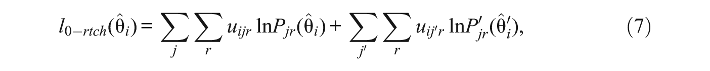
Unlike the procedures intended for stability designs, the procedures proposed in this section are based on separate ML trait estimates ( ${\hat{θ}}_{i} and {\hat{θ}}_{i}'$ ), which are obtained from the Time 1 and Time 2 patterns on the basis of the invariant item parameters. So, the log-likelihood retest index in this case is

l_{0 - r t c h} ({\hat{θ}}_{i}) = \sum_{j} \sum_{r} u_{i j r} ln P_{j r} ({\hat{θ}}_{i}) + \sum_{j'} \sum_{r} u_{i j' r} ln P_{j r}' ({\hat{θ}}_{i}'),

with mean and variance

\begin{array}{l} E (l_{0 - r t c h} ({\hat{θ}}_{i})) = E (l_{0} ({\hat{θ}}_{i})) + E (l_{0} ({\hat{θ}}_{i}')), \\ V a r (l_{0 - r t c h} ({\hat{θ}}_{i})) = V a r (l_{0} ({\hat{θ}}_{i})) + V a r (l_{0} ({\hat{θ}}_{i}')) . \end{array}

And the proposed standardized index is

l_{z - r t c h} = \frac{l_{0 - r t c h} - E (l_{0 - r t c h})}{\sqrt{V a r (l_{0 - r t c h})}} .

Drasgow et al. (1991) proposed a multidimensional extension of the l_z index intended for a “multi-unidimensional” test: a test consisting of a series of unidimensional blocks or scales in which the traits underlying each scale are generally correlated. Under the additional assumptions described above, the present proposal can be viewed methodologically as the particular case of Drasgow et al.’s proposal in which: (a) there are two blocks of unidimensional item scores (i.e., the scores at Time 1 and the scores at Time 2), (b) each block depends on a different trait (θ_i and θ′_i), and (c) the traits are possibly correlated. Indeed, the results in (7) and (8) agree with those obtained by Drasgow et al.: (a) the multidimensional unstandardized log-likelihood index is the sum of the unidimensional indices and (b) the mean and variance of l₀ is the sum of the unidimensional means and variances, respectively.

The reference distribution for l_z-rtch is again the standard normal, and according to asymptotic theory, its empirical distribution under the null hypothesis of consistency is expected to be closer to the reference distribution than in the case of the index based on a single test administration. Also, for the same reasons discussed above, the index based on the extended pattern of 2n responses is expected to be more powerful than the index based on a single administration.

Finally, as in the case of the stability procedure, if a pattern is flagged as potentially inconsistent by the overall index, further information about the sources of misfit can be gained by separately computing the standard l_z statistic (2) at Time 1 and Time 2. Note, however, that, unlike the stability procedure, in this case each separate statistic is based on a different trait estimate.

Some Practical Considerations

This section discusses the conditions in which the procedures proposed in the article are expected to work appropriately in real applications. The discussion is organized around two main points: (a) fulfillment of the basic assumptions and (b) test characteristics. The discussion is expected to provide some general guidelines for the potentially interested researcher.

The procedures proposed so far are based on three main assumptions: (a) the item parameters are taken as fixed and known, (b) they are assumed to be the same at Time 1 and Time 2, and (c) the local independence principle holds for repeated item measurements. The last assumption is related to an additional procedure proposed in the article and is discussed separately in the next section.

The assumption of known item parameters is approximately satisfied in practice if a calibrated item set (obtained from previous studies) is available. This situation is not unusual in many IRT applications. In the other cases, however, the item parameters are not known and must be estimated in the sample (in the present proposal the estimation is generally based on the Time 1 data). If this is the case, the most important recommendation is to first assess the overall fit of the chosen IRT model before (a) obtaining the trait estimates and (b) undertaking the person-fit assessment (Ferrando, in press; Meijer & Tendeiro, 2012). This is because, if the IRT model fails to provide an acceptable fit to the data, then the misfit of an individual response pattern does not necessarily indicate inconsistent responding; it might indicate general misfit of the model, individual inconsistency, or both.

The conceptual meaning of the second assumption—the invariance of the item parameters over time—is that the measurement characteristics of the items are the same at Time 1 and Time 2. This assumption, which is known as stationarity, is generally adopted in most longitudinal models (e.g., Kenny & Campbell, 1989) and is considered to be reasonable when the instrument that is administered on both occasions is the same (as in the present proposal). Furthermore, if the chosen IRT model can be parameterized as a factor-analytic model (both the 2PM and the GRM can), the stationarity assumption can be tested by fitting a two-wave model and imposing successive invariance restrictions (see Ferrando, 2002).

In any discussion of the test characteristics that are appropriate for the present proposals, all the L-B procedures must first be regarded as two-stage: The same response pattern is used to (a) obtain the trait estimate and (b) compute the person-fit index based on this estimate. Viewed in this way, it is clear that if the trait estimate is not accurate, the person-fit index will not be either. In a different context, Emons, Sijtsma, and Meijer (2007) found that for both binary and graded-response models, it was hard to obtain accurate trait estimates with a test containing fewer than 20 items. This is particularly relevant when the trait estimates are ML (as assumed in this article) because they are prone to some instability at the extremes (e.g., Zimowski et al., 2003).

It is more demanding to make an accurate estimation of an L-B index than a trait level (Ferrando, in press). Many factors are involved: type of misfit, item format, number of items, spread of item locations, and amount of item discrimination (Nering, 1995; Reise, 1995). So, it is hard to make recommendations. The simulation study and the empirical illustrations below aim to provide additional information. For the moment, however, in favorable conditions (moderate to high discrimination and a good spread of item difficulties) it is recommended not to use the proposed procedures with fewer than 20 items. In more detail, for the stability-based procedures, which jointly use the Time 1 and Time 2 responses to estimate θ, a bare recommended minimum would be a 10-item test. The change-based procedures would require tests containing 20 or more items.

Addressing Retest Effects

Retest effects can be defined as the tendency for individuals to duplicate their former item responses (Morrison, 1981). This tendency might be due to memory effects or due to incidental item features that tend to elicit the same response on each occasion (Thorndike, 1951). From an IRT point of view, the existence of retest effects is a case of positive local dependence and so violates the assumption of conditional independence under repetition on which the procedures proposed in this article are based. This section (a) discusses the impact of retest effects on l_z-rts and l_z-rtch and (b) proposes a procedure to identify possible retest effects at the individual level.

The presence of retest effects is mainly expected to affect both l_z-rts and l_z-rtch, and the expected type of impact is an outward bias on the corresponding estimates. The rationale is as follows. If the individual responds consistently at Time 1 and tends to duplicate responses at Time 2, then the total statistic would tend to flag this individual as more consistent than he/she really is. Conversely, inconsistent responding at Time 1 and retest effects would lead to the individual being flagged as more inconsistent than he/she really is.

The procedure proposed in this section is intended to identify retest effects at the level of each individual response pattern. It is a modification of a statistic that was proposed as a means of identifying local dependence at the item level.

The statistic Q3 (Yen, 1984) is the correlation of residuals over respondents for the pair of items that are assessed for local dependence. It is very simple, appears to work well, and offers a reasonable compromise between maximum power and minimum false-positive rate (Kim, De Ayala, Ferdous, & Nering, 2011). In the present proposal, which is intended at the individual level, (a) the residuals are obtained over items at both points in time for a given individual and (b) the initial Q3 proposal, which was solely intended for binary responses, is extended to the graded response case. First, the residuals at Time 1 and Time 2 are defined as

d_{i j} = X_{i j} - E (X_{i j} | {\hat{θ}}_{i}), d_{i j}' = X_{i j}' - E (X_{i j}' | {\hat{θ}}_{i}')

(note that in the stability case ${\hat{θ}}_{i} = {\hat{θ}}_{i}'$ ). The proposed statistic rt-Q3 corresponding to individual i is the product–moment correlation between the residuals d and d′ obtained over the j = 1, . . ., n items. The expectation in (10) is given by (e.g., Chang & Mazzeo, 1994).

E (X_{i j} | {\hat{θ}}_{i}) = \sum_{r} r P_{j r} ({\hat{θ}}_{i}) .

The main limitation of the original Q3 index is the lack of a clear reference distribution for establishing cutoff values (Kim et al., 2011). To solve this problem, the approach proposed here for rt-Q3 is to establish cutoff values by using simulation. In greater detail, for the stability case, the simple approach for a given data set is to (a) take the item parameters as fixed; (b) draw a large number of θ values from the standard normal distribution; (c) simulate a locally independent pair of response patterns (i.e., test and retest) for each θ value on the basis of the fixed item parameters; (d) compute the values of rt-Q3 and determine their distribution; and (e) obtain the cutoff values, which will be the same for all simulees. If the rt-Q3 value of a respondent is above the upper cutoff value, then retest effects may have been operating in his/her responses at Time 2. In the change case, the procedure is the same except that a pair of different values is now obtained in Step (b): the trait level at Time 1 and the trait level at Time 2.

The proposals in this section are useful for two main reasons. First, they provide additional information about the answering behavior of the respondent at Time 2. Second, they allow the tenability of the main assumption on which the extended L-B indices proposed here are based to be examined. These points are further discussed in the illustrative examples below.

Empirical Studies

This section describes (a) a simulation study and (b) two real-data studies in the personality domain. The simulation study was preliminary and assessed the functioning of the proposed procedures under very basic conditions. The first real-data study illustrates the use of the stability procedure with a test calibrated using the GRM. The second illustrates the use of the change procedure in the case of a test composed of binary items and calibrated with the 2PM.

Simulation Study

The main purpose of the study was to assess the functioning of both the stability procedure and the change procedure under two general conditions: (a) when the null hypothesis was true and (b) when the samples contained a certain proportion of inconsistent patterns. Given their preliminary nature, most basic conditions were kept as simple as possible. First, the simulated responses were binary and were fitted with the 2PM. Second, the item parameters were taken as known (as is the case when a calibrated item set is available). Third, all data sets were generated with difficulty parameters evenly spaced in the range [−2.7; 2.7] and discriminations distributed N(1; 0.1). Furthermore, in the null-hypothesis conditions, the distribution of θ was standard normal. Finally, under the alternative-hypothesis conditions, inconsistency was created by randomly responding to half of the test items. This was done because random responding is an overall type of misfit that is generally well detected by L-B indices (Ferrando, in press). Overall, it should be noted that (a) even under all these simplified conditions the study was relatively complex and (b) it was intended to provide some clear initial results that could serve as a basis for future studies.

The common independent variables were test length and sample size. Furthermore, the simulations based on the alternative-hypothesis conditions used a third variable: the proportion of inconsistent patterns in the sample. In all cases, two levels of sample size were considered: N = 200 (a small sample) and N = 400 (medium sample). Test lengths were n = 10, n = 20, and n = 30 for the stability assessments and n = 20 and n = 30 for the change assessments. As discussed below, the shortest level in both cases is a recommended minimum, whereas a 30-item set would be considered as medium-long. Finally, two proportions of inconsistent patterns were considered: 10% and 30%. As a summary, simulations under the null-hypothesis condition used fully crossed 3 × 2 (stability) and 2 × 2 (change) designs, whereas simulations under the alternative hypothesis used 3 × 2 × 2 (stability) and 2 × 2 × 2 (change) designs. In all cases, the result that is reported in each cell is the average obtained across 10 replications.

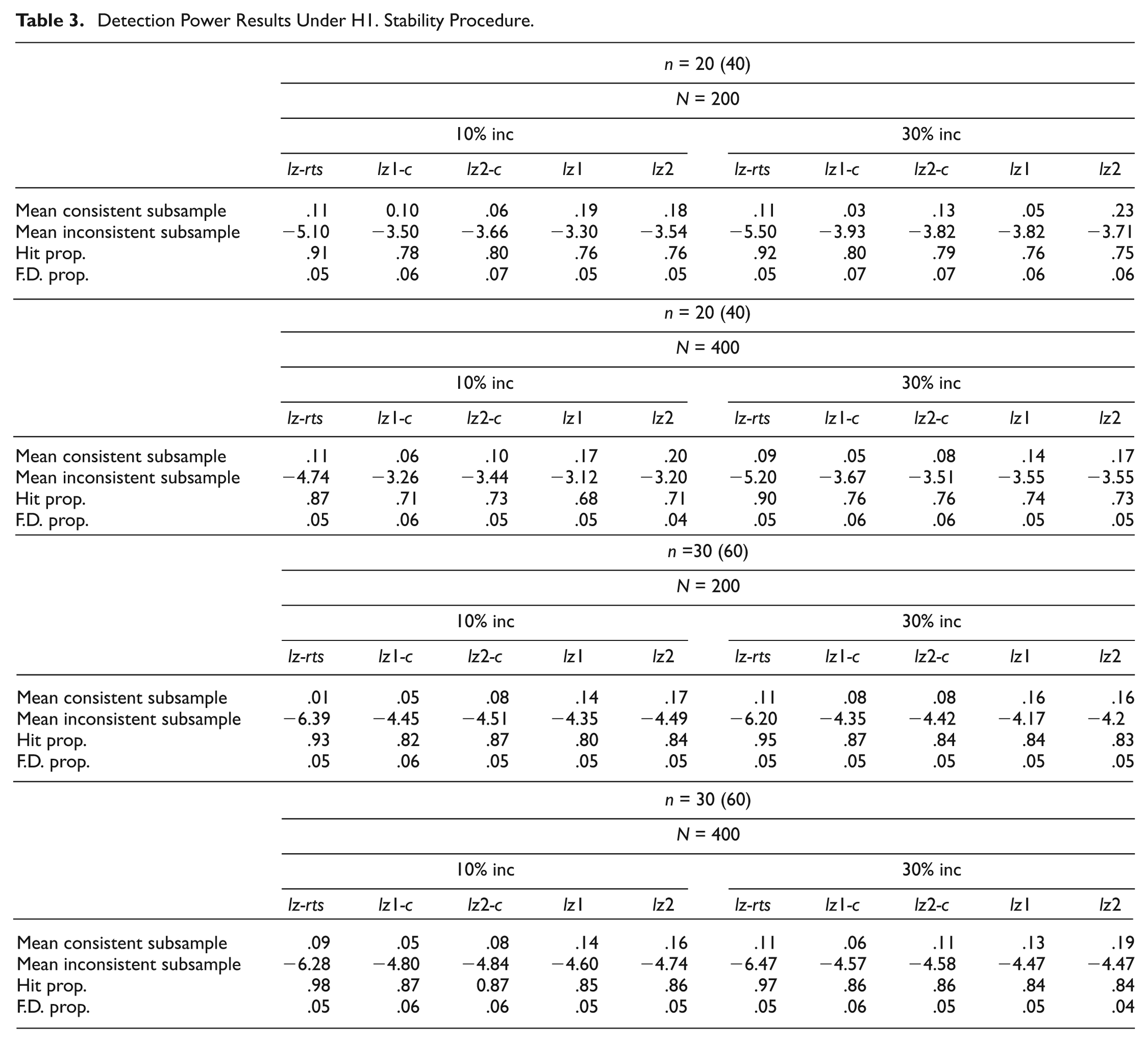
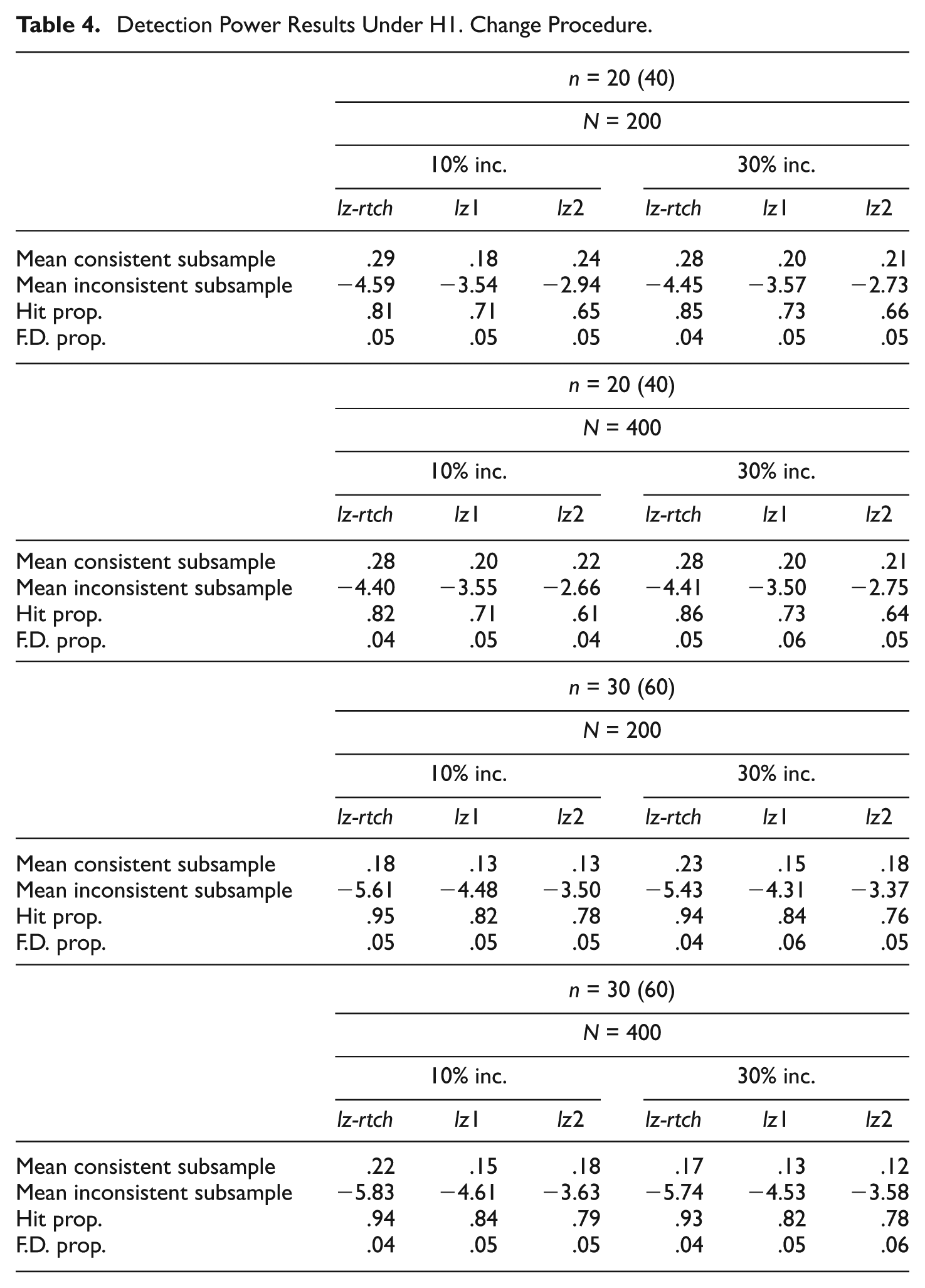
In the stability-based simulations, the indices that were assessed were (a) l_z-rts, (b) l_z at Time 1 and l_z at Time 2 based on the common trait estimate (l_z₁-c and l_z₂-c), and (c) l_z at Time 1 and l_z at Time 2 based on the separate trait estimates (l_z₁ and l_z₂). The last two indices were included so that the potential advantages of estimating θ based on the double 2n pattern could be assessed. In the change-based simulations the indices were (a) l_z-rtch and (b) l_z at Time 1 and l_z at Time 2 based on the separate trait estimates (l_z₁ and l_z₂). Because the binary responses allow it, in all cases Snijders’s (2001) correction was used when computing the indices (see Magis, Raîche, & Béland, 2012).

In accordance with the discussion above, the main interest in the null-hypothesis simulations was to assess the adherence of the empirical distributions to the standard normal distribution. In contrast, the main interest in the alternative-hypothesis simulations was to assess detection power. So, the dependent variables were different in both cases. In the first case they were (a) mean value, (b) standard deviation, (c) skewness, (d) Kolmogorov–Smirnov (K-S) statistic and associated probability, and (e) empirical Type I error using a cutoff value of z_c = −1.65 (which corresponds to a nominal level of 0.05 in the standard normal distribution). In the second case, the dependent variables were (a) means and (b) standard deviations in the consistent and inconsistent subsamples, (c) proportion of hits (inconsistent patterns detected as such), and (e) proportion of false detections (consistent patterns detected as inconsistent). The results are shown in Tables 1 to 4.

Table 1.

Normal Approximation Results Under the Null Hypothesis. Stability Procedure.

	n = 10 (20)
	N = 200					N = 400
	lz-rts	lz1-c	lz2-c	lz1	lz2	lz-rts	lz1-c	lz2-c	lz1	lz2
Mean	.17	.14	.11	.29	.26	.21	.16	.14	.30	.29
SD	.97	.97	.96	.94	.94	.96	.96	.94	.94	.91
Skewness	−1.02	−1.80	−1.45	−1.73	−1.53	−1.10	−1.68	−1.53	−1.74	−1.59
KS-distance	0.11	0.18	0.19	.25	0.24	.11	.19	0.18	.25	.25
KS-p	.02	.00	.00	.00	.00	.01	.00	.00	.00	.00
Empirical Type I error (−1.65)	.05	.06	.06	.05	.04	.05	.06	.06	.04	.04

	n = 20 (40)
	N = 200					N = 400
	lz-rts	lz1-c	lz2-c	lz1	lz2	lz-rts	lz1-c	lz2-c	lz1	lz2
Mean	.11	.07	.09	.17	.19	.12	.07	.10	.17	.20
SD	1.00	.99	.99	.97	.98	1.00	1.00	1.01	.97	.99
Skewness	−.70	−1.07	−1.02	−1.02	−1.08	−.63	−1.06	−1.14	−1.02	−1.11
KS-distance	.07	.10	−.10	.11	.11	.06	.09	.10	.10	.11
KS-p	.31	.07	.06	.05	.03	.16	.00	.00	.00	.00
Empirical Type I error (−1.65)	.05	.06	.06	.05	.05	.05	.06	.07	.05	.06

	n = 30 (60)
	N = 200					N = 400
	lz-rts	lz1-c	lz2-c	lz1	lz2	lz-rts	lz1-c	lz2-c	lz1	lz2
Mean	.14	.08	.12	.16	.20	.12	.06	.11	.14	.19
SD	1.00	1.00	1.00	.99	.98	1.00	1.00	.98	1.00	.96
Skewness	−.63	−.93	−.90	−.88	−.88	−.61	−.92	−.91	−.94	−.91
KS-distance	.06	.08	.08	.08	.09	.05	.07	.07	.08	.07
KS-p	.49	.21	.17	.12	.17	.30	.07	.05	.04	.06
Empirical Type I error (−1.65)	.05	.06	.06	.05	.04	.05	.07	.05	.06	.04

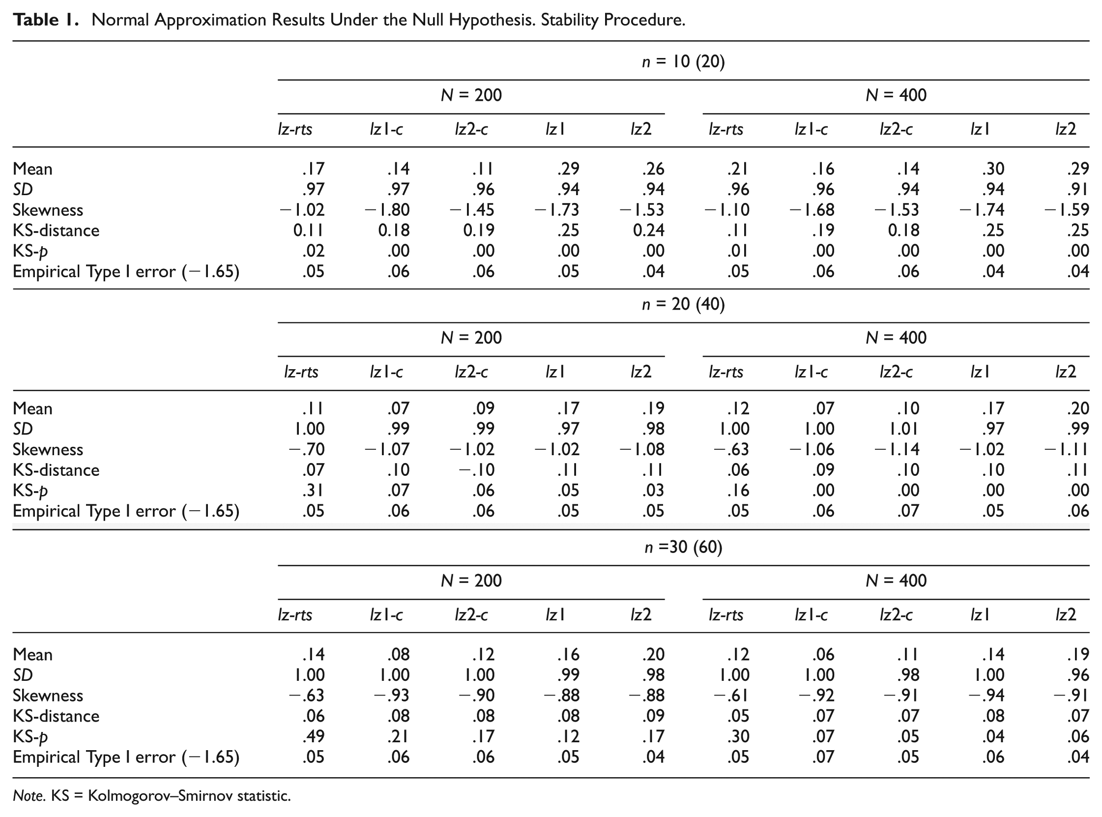
Note. KS = Kolmogorov–Smirnov statistic.

Table 2.

Normal Approximation Results Under the Null Hypothesis. Change Procedure.

	n = 20 (40)						n = 30 (60)
	N = 200			N = 400			N = 200			N = 400
	lz-rtch	lz1	lz2	lz-rtch	lz1	lz2	lz-rtch	lz1	lz2	lz-rtch	lz1	lz2
Mean	.24	.19	.17	.30	.28	.21	.22	.16	.15	.22	.18	.14
SD	.98	.98	.99	.97	.95	.96	.98	.98	.98	.98	.95	.99
Skewness	−.64	−1.04	−1.10	−.79	−1.13	−1.02	−.51	−.88	−.92	−.56	−.74	−.86
KS-distance	.07	.11	.11	.06	.11	.10	.05	.09	.08	.05	.07	.07
KS-p	.29	.03	.03	.15	.01	.01	.53	.12	.22	.30	.08	.07
Empirical Type I error (−1.65)	.05	.05	.05	.04	.04	.05	.04	.05	.06	.04	.04	.05

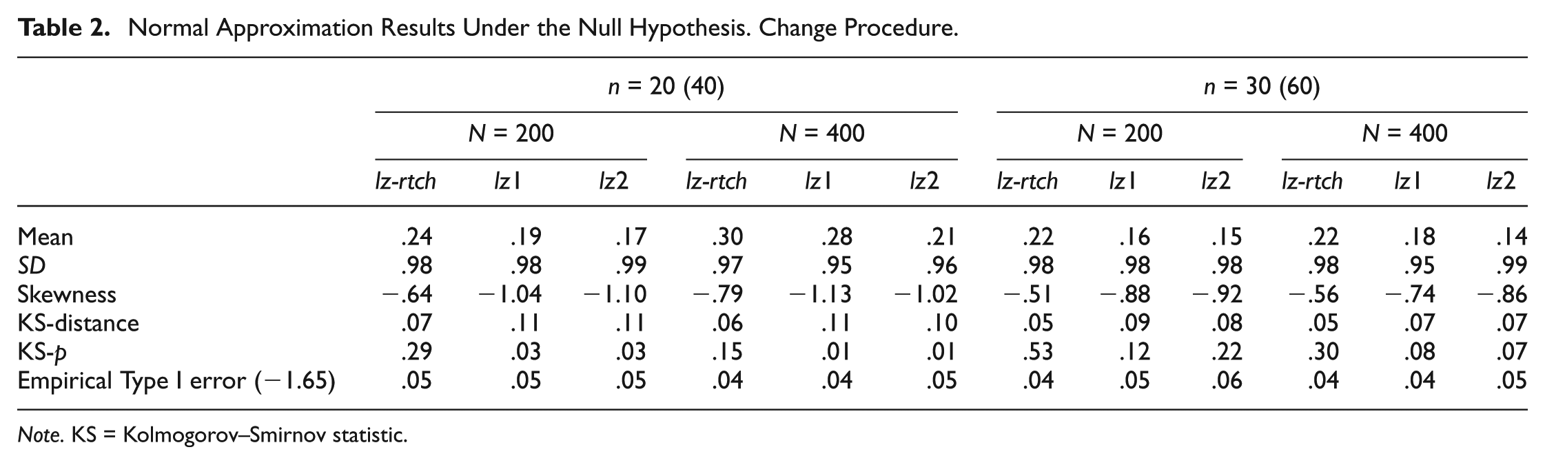
Note. KS = Kolmogorov–Smirnov statistic.

Table 3.

Detection Power Results Under H1. Stability Procedure.

	n = 20 (40)
	N = 200
	10% inc					30% inc
	lz-rts	lz1-c	lz2-c	lz1	lz2	lz-rts	lz1-c	lz2-c	lz1	lz2
Mean consistent subsample	.11	0.10	.06	.19	.18	.11	.03	.13	.05	.23
Mean inconsistent subsample	−5.10	−3.50	−3.66	−3.30	−3.54	−5.50	−3.93	−3.82	−3.82	−3.71
Hit prop.	.91	.78	.80	.76	.76	.92	.80	.79	.76	.75
F.D. prop.	.05	.06	.07	.05	.05	.05	.07	.07	.06	.06

	n = 20 (40)
	N = 400
	10% inc					30% inc
	lz-rts	lz1-c	lz2-c	lz1	lz2	lz-rts	lz1-c	lz2-c	lz1	lz2
Mean consistent subsample	.11	.06	.10	.17	.20	.09	.05	.08	.14	.17
Mean inconsistent subsample	−4.74	−3.26	−3.44	−3.12	−3.20	−5.20	−3.67	−3.51	−3.55	−3.55
Hit prop.	.87	.71	.73	.68	.71	.90	.76	.76	.74	.73
F.D. prop.	.05	.06	.05	.05	.04	.05	.06	.06	.05	.05

	n = 30 (60)
	N = 200
	10% inc					30% inc
	lz-rts	lz1-c	lz2-c	lz1	lz2	lz-rts	lz1-c	lz2-c	lz1	lz2
Mean consistent subsample	.01	.05	.08	.14	.17	.11	.08	.08	.16	.16
Mean inconsistent subsample	−6.39	−4.45	−4.51	−4.35	−4.49	−6.20	−4.35	−4.42	−4.17	−4.2
Hit prop.	.93	.82	.87	.80	.84	.95	.87	.84	.84	.83
F.D. prop.	.05	.06	.05	.05	.05	.05	.05	.05	.05	.05

	n = 30 (60)
	N = 400
	10% inc					30% inc
	lz-rts	lz1-c	lz2-c	lz1	lz2	lz-rts	lz1-c	lz2-c	lz1	lz2
Mean consistent subsample	.09	.05	.08	.14	.16	.11	.06	.11	.13	.19
Mean inconsistent subsample	−6.28	−4.80	−4.84	−4.60	−4.74	−6.47	−4.57	−4.58	−4.47	−4.47
Hit prop.	.98	.87	0.87	.85	.86	.97	.86	.86	.84	.84
F.D. prop.	.05	.06	.06	.05	.05	.05	.06	.05	.05	.04

Table 4.

Detection Power Results Under H1. Change Procedure.

	n = 20 (40)
	N = 200
	10% inc.			30% inc.
	lz-rtch	lz1	lz2	lz-rtch	lz1	lz2
Mean consistent subsample	.29	.18	.24	.28	.20	.21
Mean inconsistent subsample	−4.59	−3.54	−2.94	−4.45	−3.57	−2.73
Hit prop.	.81	.71	.65	.85	.73	.66
F.D. prop.	.05	.05	.05	.04	.05	.05

	n = 20 (40)
	N = 400
	10% inc.			30% inc.
	lz-rtch	lz1	lz2	lz-rtch	lz1	lz2
Mean consistent subsample	.28	.20	.22	.28	.20	.21
Mean inconsistent subsample	−4.40	−3.55	−2.66	−4.41	−3.50	−2.75
Hit prop.	.82	.71	.61	.86	.73	.64
F.D. prop.	.04	.05	.04	.05	.06	.05

	n = 30 (60)
	N = 200
	10% inc.			30% inc.
	lz-rtch	lz1	lz2	lz-rtch	lz1	lz2
Mean consistent subsample	.18	.13	.13	.23	.15	.18
Mean inconsistent subsample	−5.61	−4.48	−3.50	−5.43	−4.31	−3.37
Hit prop.	.95	.82	.78	.94	.84	.76
F.D. prop.	.05	.05	.05	.04	.06	.05

	n = 30 (60)
	N = 400
	10% inc.			30% inc.
	lz-rtch	lz1	lz2	lz-rtch	lz1	lz2
Mean consistent subsample	.22	.15	.18	.17	.13	.12
Mean inconsistent subsample	−5.83	−4.61	−3.63	−5.74	−4.53	−3.58
Hit prop.	.94	.84	.79	.93	.82	.78
F.D. prop.	.04	.05	.05	.04	.05	.06

For both stability and change simulations, and for all the indices, Tables 1 and 2 show a series of general results, some of which have been consistently reported in previous studies: (a) means consistently above 0.0, (b) SDs below 1.0, (c) negatively skewed distributions, and (d) adherence to the normal distribution that increases with test length (Nering, 1995; Reise, 1995; Seo & Weiss, 2013). As for the remaining general results, it is noted that no systematic differences appear at different sample sizes and, finally, that in all cases the empirical Type I error proportions are quite close to the .05 nominal level.

We turn now to more specific results under the null-hypothesis conditions. With regard to the stability procedure, it seems clear that, as expected, l_z-rts better adheres to the normal distribution than the remaining indices, especially in terms of less skewness and better K-S distances and probabilities. As was also expected, the superiority of l_z-rts increases as the test gets shorter. Regarding the single-occasion indices, l_z₁-c and l_z₂-c (which are based on the improved common estimate) tend to perform better than l_z₁ and l_z₂ although differences here are minor. Finally, because all the SDs and Type I error proportions are quite close to the reference values, no substantial differences can be found regarding these dependent variables.

These same results can be observed for the change procedure in Table 2. In this case, however, it is clear that in all conditions l_z-rtch adheres to the normal distribution better than the separate l_z₁ and l_z₂ indices.

In both the change and the stability procedure, one negative result is that the upwardly biased mean of the indices based on the full test–retest pattern is generally larger than the means of the separate indices. To address this issue analytically, the most general case in which separate trait levels are obtained is considered. According to (8) and (9), the two full test–retest indices proposed in this article, denoted generically by l_z-rt, can be written for each respondent i as

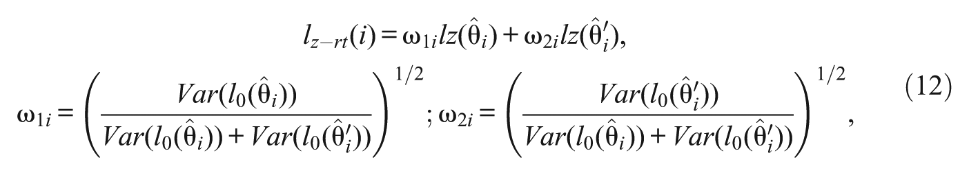
\begin{array}{l} l_{z - r t} (i) = ω_{1 i} l z ({\hat{θ}}_{i}) + ω_{2 i} l z ({\hat{θ}}_{i}'), \\ ω_{1 i} = {(\frac{V a r (l_{0} ({\hat{θ}}_{i}))}{V a r (l_{0} ({\hat{θ}}_{i})) + V a r (l_{0} ({\hat{θ}}_{i}'))})}^{1 / 2}; ω_{2 i} = {(\frac{V a r (l_{0} ({\hat{θ}}_{i}'))}{V a r (l_{0} ({\hat{θ}}_{i})) + V a r (l_{0} ({\hat{θ}}_{i}'))})}^{1 / 2}, \end{array}

that is, a weighted composite of the standardized indices computed separately at Time 1 and at Time 2. Now, in the case of l_z-rts both variances in the weight expressions are the same for each respondent, so the weight values are 0.707 (i.e, $1 / \sqrt{2}$ ) for all of them. In the case of l_z-rtch the results suggest that the variances are approximately equal, so the weight values are generally expected to be close to 0.707. Therefore, if the means of the L-B indices computed separately at Time 1 and Time 2 are both upwardly biased, then the mean of the full index is expected to be more biased than the average value of the separate means. This result suggests that future proposals for correcting the mean biases of the L-B indices are of particular interest for the procedures proposed in this article.

Results on the alternative-hypothesis conditions are in Tables 3 and 4 and, again, show certain general trends: (a) the proportion of false detections is quite close to the .05 nominal level in all cases, (b) no systematic differences appear in the different sample-size conditions, and (c) detection power increases with test length, as expected.

Differential results are clearer here than in the previous null-hypothesis conditions. In the stability procedure, the detection power of l_z-rts is substantially better than that of the single-occasion indices, and the differences become more pronounced in the case of the shortest test, as expected. Furthermore, those single-occasion indices based on the common trait estimate tend to perform better than those based on the separate estimates. Regarding the change-procedure results (Table 4), l_z-rtch performs substantially better than the separate indices in all cases.

In both stability and change procedures, it is noted that the improved performance of the test–retest indices is consistently reflected in the last three dependent variables, that is, (a) more extreme negative means in the inconsistent sub-samples and (b) a higher percentage of hits while maintaining the false detections close to the nominal level. Finally, regarding the proportion of inconsistent patterns, results tend to be slightly better in all cases in the 30% groups. However, the improvements are rather small.

Example 1. Person Fit Assessment With Graded Response Items Based on the Stability Procedure

The short Spanish version of the Indirect Aggression Scale for Aggressors (IAS-A; Anguiano-Carrasco & Vigil-Colet, 2011) is a 10-item test intended to measure social manipulation behaviors in which the aggressor acts on the people around the target with the aim of harming him/her but without having to come into direct confrontation. The IAS-A items are answered on a 5-point Likert-type scale ranging from 1 (strongly disagree) to 5 (strongly agree). In this study, the IAS-A was administered under neutral conditions to a sample of 371 undergraduate students. Of these, 156 were retested 1 month later under the same conditions. No treatment between Time 1 and Time 2 was given, and the measured trait was assumed to be stable under this retest interval. So, the stability procedure will be used here.

As discussed above, a 10-item personality scale is considered too short even for accurate trait estimation. However, the stability procedure, which is based on 20 responses, is expected (a) to provide more accurate trait estimates and (b) to provide minimally acceptable power levels for detecting inconsistency. It should be stressed again that the potentially improved trait estimate of an individual can only be validly interpreted if his/her test–retest response pattern is consistent.

Samejima’s GRM was fitted to the data in two stages. In the calibration stage, the item parameter estimates were obtained on the basis of the 371 respondents available at Time 1, and the overall model-data fit was assessed. Item discriminations and locations were calibrated using WLSM estimation as implemented in the program Mplus 6.11 (Muthén & Muthén, 2010). The overall fit of the model was quite acceptable: root mean square error of approximation = .07, Tucker–Lewis index/nonnormed fit index = .99, goodness of fit index = .99, and root mean square residuals (standardized) = .05. Given these results, the item parameters were taken as fixed and known and used to obtain ML individual estimates in the scoring stage.

The assumption of local independence was then assessed by identifying retest effects. The upper 90% cutoff value for rt-Q3 was 0.56, and 31 respondents (21% of the sample) had rt-Q3 values above this point. So, in principle, for most of the sample the local independence model can be considered to be appropriate. Finally, the person fit statistics l_z-rts, l_zc (Time 1), and l_zc (Time 2) were computed for each individual. As expected, the distribution of the l_z-rts values had a slight negative skew, with a heavier left tail. The mean and standard deviation were −0.17 and 0.99 and are quite close to the standard normal reference values. In view of this result, a (−2; 2) confidence band was next chosen to judge a respondent as potentially overconsistent (above 2) or inconsistent (below −2). As for the upper tail, only 3 respondents (1.9%) had l_z-rts values above 2, which is quite close to the 2.2% nominal level expected under the null hypothesis of no misfit. The results for these respondents are in the upper panel of Table 5. Note that two respondents have near-zero rt-Q3 values. So the most likely interpretation is simply that they answered the items consistently at both points in time. The rt-Q3 value for the third individual suggests strong retest effects. So, her l_z-rts value of 2.2 is possibly outwardly biased, and she probably did not respond as consistently as the person-fit index suggests.

Table 5.

Person-Fit Results for the Most Overconsistent and Inconsistent Patterns. Illustrative Example 1.

Respondent no.	l_z-c (T1)	l_z-c (T2)	l_z-rts	rt-Q3
(a) Overconsistent
30	2.21	1.34	2.52	0.01
28	1.87	1.65	2.49	0.01
20	1.73	1.37	2.20	0.79
(b) Inconsistent
98	−4.52	−0.30	−3.41	0.01
51	−0.11	−3.34	−2.40	−0.10

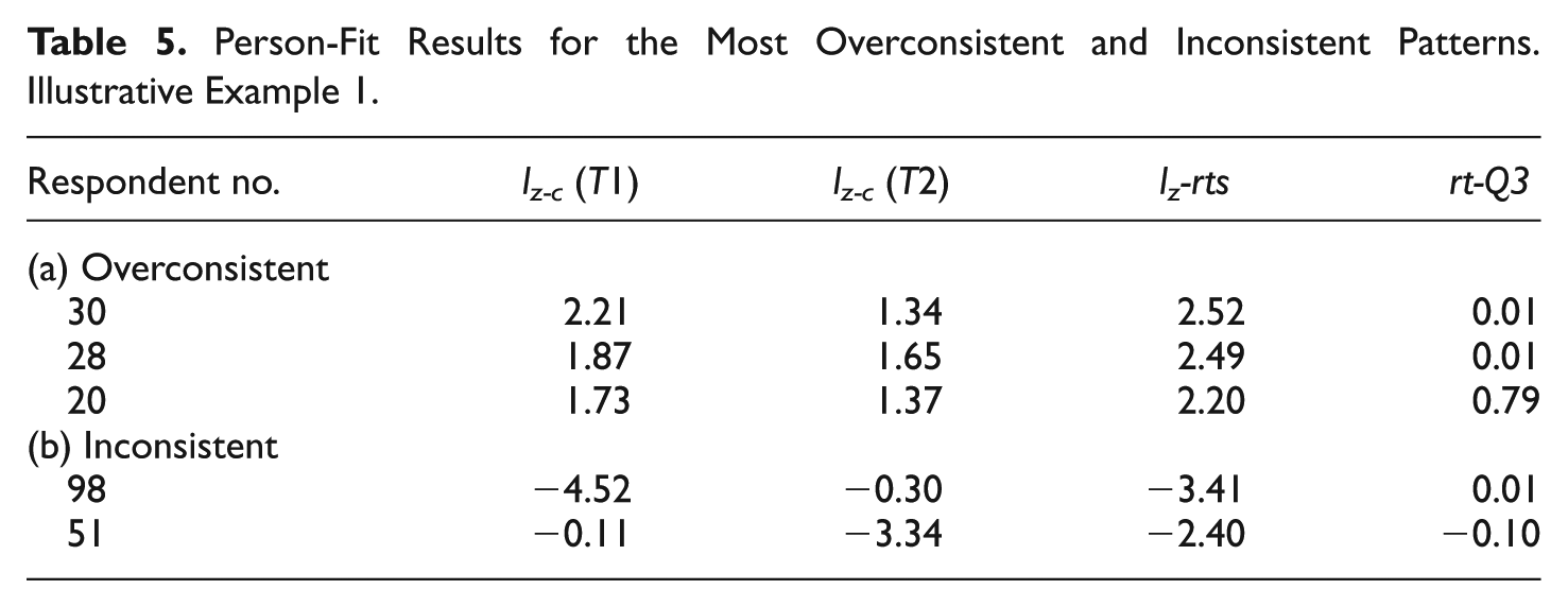
In accordance with the heavier left tail, 12 individuals (7.7%) fell below the lower −2 cutoff point, a percentage that is clearly larger than the expected 2.2% nominal level. For illustrative purposes, the results of two of these individuals, which are shown in the lower panel of Table 5, are now discussed. The overall results for Respondent 98 suggest that this individual responded inconsistently and that the detected inconsistency was not exaggerated by retest effects. The separate l_z values suggest that most of the inconsistent responding took place in the first administration. A single-response residual analysis (see Ferrando, in press) suggested that this respondent provided inconsistent responses to 4 of the 10 items at Time 1 whereas no inconsistent responses were found at Time 2.

The l_z-rts and rt-Q3 values of respondent 51 lead to the same overall interpretation as Respondent 98. The separate l_z indices, however, lead to opposite results. So, in this case inconsistency seems to be due to the retest responses. Residual analysis suggested that this respondent provided one inconsistent response at Time 1 and three inconsistent responses at Time 2.

Example 2. Person Fit Assessment With Binary Items Based on the Change Procedure

The measure used here was the Psychoticism (P) scale of the Eysenck Personality Questionnaire revised (EPQ-R; Eysenck, Eysenck, & Barrett, 1985), which is made up of 32 binary items. The EPQ-R was administered on two occasions with a retest interval of 6 weeks in all cases. At Time 1 the participants were asked to respond under the standard instructions provided in the manual. At Time 2 they received faking-inducing instructions (try to give a good impression so that you will be given a job you really want). A high P level is clearly considered to be highly socially undesirable. So, the instructions were expected to produce a general decrease in the P scores at Time 2 to reflect a faked, more socialized behavior. Given the design used in this example, the change procedure seems to be the most appropriate.

In the data used here, 332 respondents completed the questionnaire at Time 1, and 277 respondents participated in both administrations. The P items were calibrated according to the 2PM by using the Time 1 data. Given that the test in this case is rather long, the calibration used simple ULS estimation. The fit was considered to be acceptable: goodness of fit index = .90 and standardized root mean square residual = .07. Next, the item parameters were taken as fixed and known and used to score individuals. Once the ML estimates had been obtained, the assumption of local independence was tested. In this case the upper 90% cutoff value for rt-Q3 was 0.30, and 80 respondents (29% of the sample) had rt-Q3 values above this point.

Table 6 shows the descriptive statistics for (a) the ML trait estimates obtained at Time 1 and Time 2 and (b) the person fit statistics: l_z-rtch, l_z (Time 1), and l_z (Time 2).

Table 6.

Descriptive Statistics for Trait Estimates and Person Fit Indices. Illustrative Example 2.

	$\hat{θ}$	$\hat{θ}'$	l_z (T1)	l_z (T2)	l_z-rtch
Mean	−0.23	−1.74	0.14	0.02	0.12
SD	1.41	1.93	0.83	0.82	0.90
Skewness	−0.80	0.27	−1.60	−1.68	−1.38

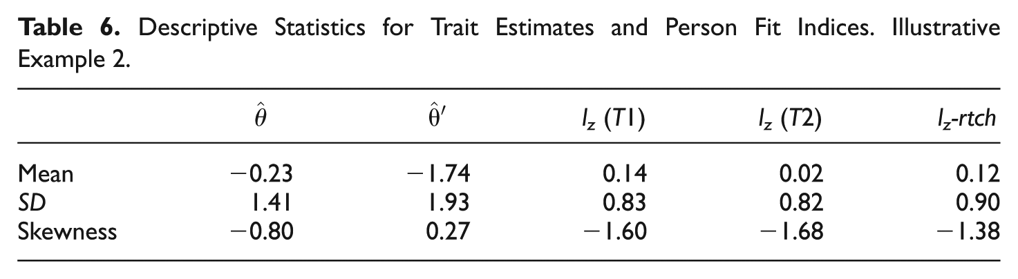
The appropriateness of the change procedure was assessed by using the confidence interval decision rule proposed by Kim-Kang and Weiss (2007). First, the proposal was adapted to the mean change case. The 95% confidence intervals for the mean estimates in Table 6 were (−0.397; −0.063) at Time 1 and (−1.967; −1.513) at Time 2, clearly nonoverlapping (Cohen’s d effect size measure was 0.90). Second, individual confidence intervals around the trait estimate were computed for each respondent. The number of nonoverlapping intervals was 151 (55%). This result, together with the fact that most changes were in the expected direction, supports the appropriateness of the change procedure.

As for the person-fit results, in all three cases the distributions had the expected negative skews, upwardly biased means, and standard deviations below the unit reference value. Note that, as expected, the mean of l_z-rtch is larger than the average of the separate-occasion means. However, the skewness is lower, and the standard deviation is closer to 1.

As in the previous example, a (−2; 2) confidence band was chosen next. As for the upper tail, no respondent had l_z-rtch values above 2, and only six individuals fell below the −2 cutoff point, a percentage that almost corresponds to the 2.2% expected under the null hypothesis of no misfit. For illustrative purposes, however, one case in which the inconsistency seems to be clear is now discussed. Table 7 summarizes the results for Respondent 165.

Table 7.

Summary of Results for Respondent 165. Illustrative Example 2.

$\hat{θ}$	$\hat{θ}'$	l_z (T1)	l_z (T2)	l_z-rtch	rt-Q3
1.34	2.92	0.22	−5.01	−3.25	0.10

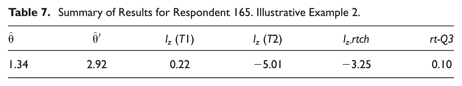
The overall results in Table 7 suggest that the full 64-response pattern of this individual was inconsistent and that the inconsistency was not exaggerated by retest effects. Furthermore, the separate l_z values suggest that this respondent was consistent at Time 1 but highly inconsistent at Time 2 and the trait estimates add more information. The trait level estimate was rather high at Time 1 and, at Time 2, instead of decreasing (which was the general trend) it increased dramatically. This change in the opposite direction suggests that the source of misfit was deliberate sabotaging, and a detailed graphical analysis (see Ferrando, in press) provided additional evidence in this direction. At Time 1, the responses of this individual agreed well with the normative item ordering. However, under the faking instructions given at Time 2, he systematically responded opposite to the normative item ordering, disagreeing with the most frequently endorsed items, and agreeing with the less frequently endorsed ones. Given the detected inconsistency of this pattern, the change estimate for Respondent 165 cannot be validly interpreted.

Discussion

IRT modeling of test–retest data can provide improved, more accurate trait estimates (in a stability study) or change estimates (in a change study). These estimates, however, can only be validly interpreted if the pattern of responses from which they are obtained is consistent with the IRT model. An additional advantage of IRT is that this necessary individual consistency can also be assessed by using person-fit indices. So far, however, person-fit developments intended for test–retest data appear to be virtually nonexistent.

The developments proposed in this article constitute an integrated approach that can be used with the two general assumptions found in applications: stability and change for a wide array of IRT models. This approach consists of two groups of procedures: (a) overall L-B indices based on the full test–retest pattern and (b) partial L-B indices intended to provide additional information about the location and sources of misfit. Furthermore, because the overall procedures assume local independence under repetition, a statistic for assessing the presence of retest effects at the individual level is also proposed.

The proposals made in this article were assessed using simulation and put into practice with two empirical studies. The simulation study was preliminary and operated under highly simplified and ideal conditions. So, the results can only be considered as a basis. In spite of this limitation, however, they were generally positive and suggest that, when compared to the single-occasion indices, the overall indices (a) tend to adhere better to the standard normal distribution under the null hypothesis of consistency and (b) are substantially more powerful for detecting inconsistency. At the same time, the simulation indicates a potential shortcoming: the use of the overall indices is expected to amplify the upward mean bias that is commonly observed in the single-occasion indices. So, the procedures that aim to correct this bias, or the use of empirical reference distributions based on Monte Carlo simulations such as those proposed in Seo and Weiss (2013) warrant further study. Overall, further simulation is clearly needed in different scenarios, for example, (a) when the item parameters are not known and must be estimated in the sample, (b) when the item characteristics are not so “ideal,” or (c) when trait estimates other than ML (e.g., Bayesian or robust estimates) are used. The sensitivity of the proposed indices for detecting different sources of misfit (e.g., cheating, extreme responding) should also be explored.

The empirical studies are not mere “ad hoc” illustrations but real applications in personality measurement, and in both cases the results obtained are meaningful. However, it is clearly acknowledged that results from only two studies are hardly generalizable and that further research based on real data is also needed. A key issue in this future research would be to explore the behavior of the proposal in different domains of measurement (ability, attitudes, etc.).

In conclusion, in spite of its limitations, the present proposal addresses a type of assessment that is clearly necessary, seems to work well (at least initially), and is expected to be a useful tool for applied researchers. The proposed procedures are relatively simple to use and can be easily programmed. However, widespread use of any proposal such as the present one needs a free user-friendly program. This is also an aim for the future.

Footnotes

Declaration of Conflicting Interests

The author(s) declared no potential conflicts of interest with respect to the research, authorship, and/or publication of this article.

Funding

The author(s) disclosed receipt of the following financial support for the research, authorship, and/or publication of this article: The research was supported by a grant from the Spanish Ministry of Economy and Competitiveness (PSI2011-22683).

References

Anguiano-Carrasco

Vigil-Colet

(2011). Assessing indirect aggression in aggressors and targets: Spanish adaptation of the Indirect Aggression Scales. Psicothema, 23, 146-152.

Baker

F. B.

Kim

(2004). Item response theory. Parameter estimation techniques (2nd ed.). New York, NY: Marcel Dekker.

Chang

Mazzeo

(1994). The unique correspondence of the item response function and item category response function in polytomously scored item response models. Psychometrika, 59, 391-404.

Drasgow

Levine

M. V.

McLaughlin

M. E.

(1987). Detecting inappropriate test scores with optimal and practical appropriateness indices. Applied Psychological Measurement, 11, 59-79.

Drasgow

Levine

M. V.

McLaughlin

M. E.

(1991). Appropriateness measurement for some multidimensional test batteries. Applied Psychological Measurement, 15, 171-191.

Drasgow

Levine

M. V.

Williams

E. A.

(1985). Appropriateness measurement with polychotomous item response models and standardized indices. British Journal of Mathematical and Statistical Psychology, 38, 67-86.

Emons

W. H. M.

Sijtsma

Meijer

R. R.

(2007). On the consistency of individual classification using short scales. Psychological Methods, 12, 105-120.

Eysenck

S. B. G.

Eysenck

H. J.

Barrett

P. T.

(1985). A revised version of the Psychoticism Scale. Personality and Individual Differences, 6, 21-29.

Ferrando

P. J.

(2002). An IRT-based two-wave model for studying short-term stability in personality measurement. Applied Psychological Measurement, 26, 286-301.

10.

Ferrando

P. J.

(2010). Assessing short-term individual consistency using IRT-based statistics. Psicológica, 31, 319-334.

11.

Ferrando

P. J.

(in press). Assessing person fit in typical-response measures. In Reise

S. P.

Revicki

D. A.

(Eds.), Handbook of item response theory modeling: Applications to typical performance assessment.

12.

Finkelman

M. D.

Weiss

D. J.

Kim-Kang

(2010). Item selection and hypothesis testing for the adaptive measurement of change. Applied Psychological Measurement, 34, 238-254.

13.

Goldberg

L. R.

(1963). A model of item ambiguity in personality assessment. Educational and Psychological Measurement, 23, 467-492.

14.

Hausknecht

J. P.

Trevor

C. O.

Farrr

J. L.

(2002). Retaking ability tests in a selection setting: Implications for practice effects, training performance, and turnover. Journal of Applied Psychology, 87, 243-254.

15.

Kenny

D. A.

Campbell

D. T.

(1989). On the measurement of stability in over-time data. Journal of Personality, 57, 445-481.

16.

Kim

De Ayala

R. J.

Ferdous

A. A.

Nering

M. L.

(2011). The comparative performance of conditional independence indices. Applied Psychological Measurement, 35, 447-471.

17.

Kim-Kang

Weiss

D. J.

(2007). Comparison of computerized adaptive testing and classical methods for measuring individual change. In Weiss

D. J.

(Ed.), Proceedings of the 2007 GMAC Conference on computerized adaptive testing. Retrieved from http://www.psych.umn.edu/psylabs/catcentral/pdf%20files/cat07kim-kang.pdf

18.

Levine

M. V.

Rubin

D. B.

(1979). Measuring the appropriateness of multiple choice test scores. Journal of Educational Statistics, 4, 269-290.

19.

M. F.

Olejnik

(1997). The power of Rasch person-fit statistics in detecting unusual response patterns. Applied Psychological Measurement, 21, 215-231.

20.

Magis

Raîche

Béland

(2012). A didactic presentation of Snijders’s lz* index of person fit with emphasis on response model selection and ability estimation. Journal of Educational and Behavioral statistics, 37, 57-81.

21.

Meijer

R. R.

(2003). Diagnosing item score patterns on a test using item response theory-based person-fit statistics. Psychological Methods, 8, 72-87.

22.

Meijer

R. R.

Sijtsma

(2001). Methodology review: Evaluating person fit. Applied Psychological Measurement, 25, 107-135.

23.

Meijer

R. R.

Tendeiro

J. N.

(2012). The use of lz and lz* person-fit statistics and problems derived from model misspecification. Journal of Educational and Behavioral Statistics, 6, 758-766.

24.

Morrison

D. G.

(1981). A stochastic model for test-retest correlations. Psychometrika, 46, 143-151.

25.

Muthén

L. K.

Muthén

(2010). Mplus user’s guide (6th ed.). Los Angeles, CA: Muthén & Muthén.

26.

Nering

M. L.

(1995). The distribution of person fit using true and estimated person parameters. Applied Psychological Measurement, 19, 121-129.

27.

Nering

M. L.

Meijer

R. R.

(1998). A comparison of the person response function and the lz person-fit statistic. Applied Psychological Measurement, 22, 53-69.

28.

Reise

S. P.

(1995). Scoring method and the detection of person misfit in a personality assessment context. Applied Psychological Measurement, 19, 213-229.

29.

Reise

S. P.

Due

A. M.

(1991). The influence of test characteristics on the detection of aberrant response patterns. Applied Psychological Measurement, 15, 217-226.

30.

Reise

S. P.

Haviland

M. G.

(2005). Item response theory and the measurement of clinical change. Journal of Personality Assessment, 84, 228-238.

31.

Samejima

(1969). Estimation of latent ability using a response pattern of graded scores. Psychometrika Monograph Supplement, 17, 1-100.

32.

Seo

D. G.

Weiss

D. J.

(2013). l_z Person-fit index to identify misfit students with achievement test data. Educational and Psychological Measurement, 73, 994-1016.

33.

Shadish

W. R.

Cook

T. D.

Campbell

D. T.

(2002). Experimental and quasi-experimental designs for generalized causal inference. Boston, MA: Houghton Mifflin.

34.

Smith

R. M.

(1986). Person fit in the Rasch model. Educational and Psychological Measurement, 46, 359-372.

35.

Snijders

T. A. B.

(2001). Asymptotic null distribution of person fit statistics with estimated person parameter. Psychometrika, 66, 331-342.

36.

Thorndike

R. L.

(1951). Reliability. In Lindquist

E. F.

(Ed.), Educational measurement (pp. 560-619). Washington, DC: American Council on Education.

37.

Yen

W. M.

(1984). Effects of local item dependence on the fit and equating performance of the three-parameter logistic model. Applied Psychological Measurement, 8, 125-145.

38.

Zimowski

Muraki

Mislevy

R. J.

Bock

R. D.

(2003). BILOG-MG 3: Item analysis and test scoring with binary logistic models. Chicago, IL: Scientific Software.

A Comprehensive Approach for Assessing Person Fit With Test–Retest Data

Abstract

Keywords

Review of the Basic L-B Indices

Proposed Approach and Rationale

Proposed Procedures When Trait Stability Is Assumed

Proposed Procedures When Change Is Assumed

Some Practical Considerations

Addressing Retest Effects

Empirical Studies

Simulation Study

Example 1. Person Fit Assessment With Graded Response Items Based on the Stability Procedure

Example 2. Person Fit Assessment With Binary Items Based on the Change Procedure

Discussion

Footnotes

Declaration of Conflicting Interests

Funding

References