Multidimensional Classification of Examinees Using the Mixture Random Weights Linear Logistic Test Model

Abstract

An essential feature of the linear logistic test model (LLTM) is that item difficulties are explained using item design properties. By taking advantage of this explanatory aspect of the LLTM, in a mixture extension of the LLTM, the meaning of latent classes is specified by how item properties affect item difficulties within each class. To improve the interpretations of latent classes, this article presents a mixture generalization of the random weights linear logistic test model (RWLLTM). In detail, the present study considers individual differences in their multidimensional aspects, a general propensity (random intercept) and random coefficients of the item properties, as well as the differences among the fixed coefficients of the item properties. As an empirical illustration, data on verbal aggression were analyzed by comparing applications of the one- and two-class LLTM and RWLLTM. Results suggested that the two-class RWLLTM yielded better agreement with the empirical data than the other models. Moreover, relations between two random effects explained differences between the two classes detected by the mixture RWLLTM. Evidence from a simulation study indicated that the Bayesian estimation used in the present study appeared to recover the parameters in the mixture RWLLTM fairly well.

Keywords

mixture item response models LLTM RWLLTM multidimensional models classification Bayesian estimation

Introduction

Mixture item response models have been developed to represent the possibility that students may not be sampled from a homogeneous population, as assumed in conventional item response theory (IRT), but rather, a mixture of multiple latent subpopulations or classes. In mixture item response models, the unobserved heterogeneity of populations is investigated using latent class analysis, and observed responses within each class are modeled using IRT models. Applications of mixture item response models in educational and psychological contexts have attempted to enhance our understanding of the differences between examinees in different classes. For example, latent classes differ in their use of strategies for test items (e.g., Bolt, Cohen, & Wollack, 2001; Mislevy & Verhelst, 1990; Rost, 1990), developmental stages in task solution (e.g., Draney, Wilson, Gluck, & Spiel, 2008; Wilson, 1989), and individual differences in the presence of test speededness (e.g., Bolt, Cohen, & Wollack, 2002; De Boeck, Cho, & Wilson, 2011; Meyer, 2010).

The distinguishing features of mixture item response models are that (a) students from distinct populations are qualitatively differentiated (De Boeck, Wilson, & Acton, 2005) and (b) each person’s population membership is unknown; instead, it is a latent variable. Thus, in mixture item response models, it is very important to find discrete characteristics that define each latent class of examinees. For example, Mislevy and Verhelst (1990) developed the idea of the mixture LLTM (MixLLTM) by coupling the concept of the linear logistic test model (LLTM; Fischer, 1973) and the mixture item response model framework, more specifically by relating characteristics of each class to known features of items. In the LLTM, items are built based on item design properties using psychological and cognitive theory, or other features of the items, and then the item difficulties are explained using the design properties. As such, the LLTM is referred to as an explanatory item response model with respect to items (De Boeck & Wilson, 2004). In the MixLLTM, each class is differentiated by the way in which item properties affect item difficulties, and these differences define the meaning of latent classes.

In addition, the random weights LLTM (RWLLTM; Rijmen & De Boeck, 2002), an extension of the LLTM, allows individual differences in the extent to which the item properties determine the item difficulties. In contrast to the LLTM, which assumes that the effects of the item features are constant for all persons, in the RWLLTM, each person can have different effects of the item properties on the item difficulties through random coefficients. In this regard, the RWLLTM captures more information about the examinees than the LLTM does. Therefore, it is interesting and potentially beneficial to formulate and investigate a mixture extension of the RWLLTM (MixRWLLTM), which can take advantage of the item explanatory aspect of the LLTM and also incorporate individual differences detected by the RWLLTM to define characteristics of latent classes. Specifically, the MixRWLLTM can be employed to identify latent classes that differ in multidimensional aspects, that is, differences in a general latent trait and specific latent dimensions defined by item design features. The primary objective of the present study is to investigate the use of the MixRWLLTM to distinguish a subpopulation of examinees as well as to improve interpretations of differences among latent classes.

To this end, this article is organized as follows. First, the LLTM and the RWLLTM are briefly reviewed, and the MixLLTM is described. Based on these approaches, the MixRWLLTM, which is of major interest in the present study, is presented with respect to model specifications. Following that, we describe an estimation algorithm for the MixRWLLTM using the Markov chain Monte Carlo (MCMC) approach implemented in WinBUGS 1.4.3 (Lunn, Thomas, Best, & Spiegelhalter, 2000) for parameter estimation of the proposed models. Then, in order to show how the MixRWLLTM can be applied to an empirical example, the results of the analysis of a verbal aggression data set are presented. Finally, a simulation is conducted to assess parameter recovery and correct identification of class membership of the MixRWLLTM.

Methods

Review of the LLTM and RWLLTM

As discussed above, the LLTM is designed to help explain how item design features influence responses on tests with a prior item structure. Suppose that there are K item properties. Under the LLTM, the probability that person p gives the correct response on item i is written as

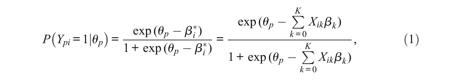
P (Y_{pi} = 1 | θ_{p}) = \frac{exp (θ_{p} - β_{i}^{*})}{1 + exp (θ_{p} - β_{i}^{*})} = \frac{exp (θ_{p} - \sum_{k = 0}^{K} X_{ik} β_{k})}{1 + exp (θ_{p} - \sum_{k = 0}^{K} X_{ik} β_{k})},

where θ_p is the latent ability of person p that follows an underlying population distribution (e.g., a normal distribution with mean zero and a constant variance) and $β_{i}^{*}$ is the difficulty of item i. As shown in Equation 1, the item difficulty in the LLTM is expressed as a function of the coefficient of property k, β_k (k = 1, . . . , K). Note that X_ik is the known value of the I× (K+1) design matrix for item i on property k. For k = 0, β₀ is the item intercept with X_i₀ = 1 for all items i, and from 1 to K, X_ik reflects the prespecified structure of composing the difficulty of item i associated with property k. Therefore, β_k represents the difficulty of property k, which corresponds to the contribution of item design feature k to the item difficulty. By taking the multilevel IRT perspective, in which the responses on items (Level 1 units) are assumed to be clustered into the persons (Level 2 units) (Adams, Wilson, & Wu, 1997), the ability θ_p can be considered as the random intercept which varies over the persons, and the item property difficulties β_k are the fixed effects which are constant across the persons.

The LLTM has the advantage of parsimony: item difficulties are explained in terms of item features and there are usually fewer item features than items. However, the assumption that item properties explain the item difficulty perfectly and that the effects of the item features are constant for all persons might be unrealistic and strict in many circumstances. The RWLLTM¹ relaxes the assumption of invariant effects of item properties by incorporating person-specific random coefficients. In detail, in the RWLLTM, person-specific random coefficients Θ_pK′ are assumed for a subset of K item properties, K′ of which coefficients are assumed to vary among persons. Therefore, X_is (s∈K′) is the element of the submatrix of the full design matrix associated with random coefficients (or random slopes) θ_ps (s∈K′). For instance, if the random coefficients are assumed for the first and second item properties among four item properties, K′ corresponds to {1, 2}, X_is is the element of the matrix consisting of the second and third columns of the full design matrix X , and Θ_pK′ = (θ_p₁, θ_p₂)′. In the RWLLTM, ∑_s∈K′X_isθ_ps is added to the difficulty of item i for person p as follows:

β_{p i}^{* *} = \sum_{k = 0}^{K} X_{i k} β_{k} + \sum_{s \in K'} X_{i s} θ_{p s} .

Alternatively, given that Θ_pK′ are the person-specific random effects, in the RWLLTM, the person ability is a multidimensional parameter, Θ_p = (θ_p₀, Θ_pK′′)′, a vector of the random intercept θ_p₀ and random coefficients θ_ps (s∈K′). Thus, the required ability for person p to respond to item i is formulated as

θ_{pi}^{*} = \sum_{s = 0}^{S} Z_{is} θ_{ps},

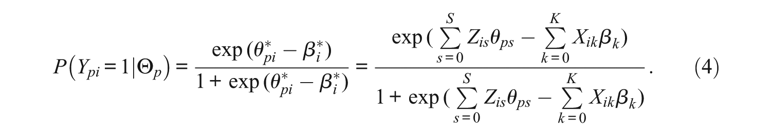
where Z_is is the value of the I× (S+1) matrix that appends a constant vector of 1 with the length of I for the random intercept θ_p₀ and submatrix of the design matrix X for the random coefficients θ_ps (s∈K′). Particularly, for s = 0, Z_i₀ = 1 for all items. For s from 1 to S, Z_is is the same as X_is (s∈K′) and S is equal to the number of random coefficients K′ (e.g., S = 2 in the above example). In the RWLLTM, the probability that person p gives the correct response on item i is written as

P (Y_{pi} = 1 | Θ_{p}) = \frac{exp (θ_{pi}^{*} - β_{i}^{*})}{1 + exp (θ_{pi}^{*} - β_{i}^{*})} = \frac{exp (\sum_{s = 0}^{S} Z_{is} θ_{ps} - \sum_{k = 0}^{K} X_{ik} β_{k})}{1 + exp (\sum_{s = 0}^{S} Z_{is} θ_{ps} - \sum_{k = 0}^{K} X_{ik} β_{k})} .

In fact, as noted by Rijmen and De Boeck (2002), the model framework Equation 4 is a special case of an earlier model, the multidimensional random coefficients multinomial logit model (MRCMLM; Adams, Wilson, & Wang, 1997), in which Z and X correspond to the scoring matrix and design matrix, respectively, of the MRCMLM. The random effects Θ_p are assumed to follow a multivariate normal distribution; therefore, the RWLLTM can be considered a multidimensional extension of the LLTM that includes additional dimensions corresponding to person-specific random effects associated with item properties.

Mixture Extensions of the LLTM and RWLLTM

The rationale for formulation of the MixLLTM is to combine the heterogeneous population from the mixture item response models and the decomposition of the item difficulties in the LLTM. In the mixture Rasch model (Rost, 1990), within each latent class, the Rasch model is assumed with class-specific person ability and class-specific item difficulty parameters. Similarly, in the MixLLTM, the LLTM is assumed to hold within each latent class. The conditional probability of the MixLLTM that person p endorses item i under the condition that this person belongs to latent class g is

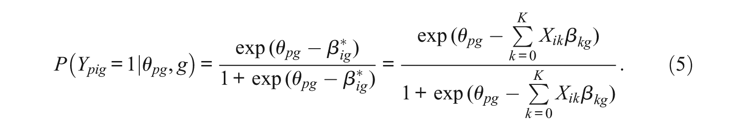
P (Y_{pig} = 1 | θ_{pg}, g) = \frac{exp (θ_{pg} - β_{ig}^{*})}{1 + exp (θ_{pg} - β_{ig}^{*})} = \frac{exp (θ_{pg} - \sum_{k = 0}^{K} X_{ik} β_{kg})}{1 + exp (θ_{pg} - \sum_{k = 0}^{K} X_{ik} β_{kg})} .

As shown in Equation 5, the conditional probability is the same as in the LLTM, but the model contains class-specific ability θ_pg and class-specific item property coefficient β_kg. In addition, the item difficulties become class-specific due to the class-specific coefficients. 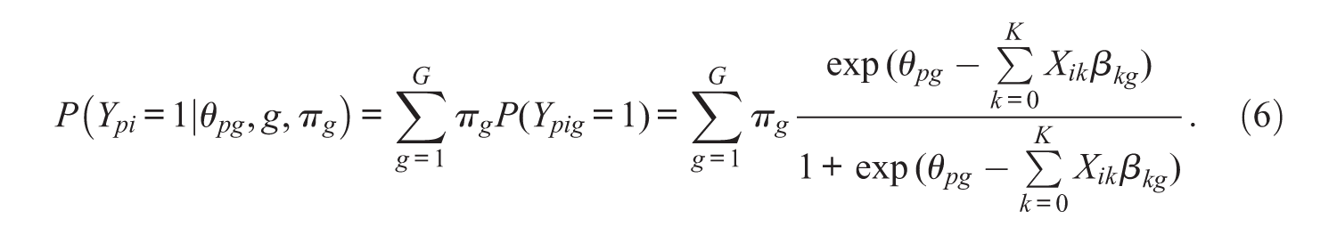It is common to assume that the ability (random intercept) follows a normal distribution with class-specific mean and variance, θ_p_g ~ N(μ_0g, $σ_{0 g}^{2}$ ) for each latent class g = 1, . . . , G. Class membership g is regarded as a latent variable with the class size parameters or the mixing proportions π_g having constraints, 0 ≤π_g≤ 1 and ∑_gπ_g = 1. Therefore, each person belongs to one of the classes with probability π_g. The marginal probability of person p’s correct response on item i in the MixLLTM is specified as

P (Y_{pi} = 1 | θ_{pg}, g, π_{g}) = \sum_{g = 1}^{G} π_{g} P (Y_{pig} = 1) = \sum_{g = 1}^{G} π_{g} \frac{exp (θ_{pg} - \sum_{k = 0}^{K} X_{ik} β_{kg})}{1 + exp (θ_{pg} - \sum_{k = 0}^{K} X_{ik} β_{kg})} .

The MixLLTM is capable of identifying distinct classes that depend on a general level of propensity, where each class is defined by class-specific ability distributions and item property parameters. However, it can be assumed that classes are also distinguished by individual differences in the degree to which item properties influence the item difficulty and in the general propensity. This goal can be achieved by extending the RWLLTM into a mixture model. Considering the model framework of the MixLLTM in Equation 6, the marginal probability that person p endorses item i in the MixRWLLTM can be represented by extending the RWLLTM in Equation 4 into a mixture model as

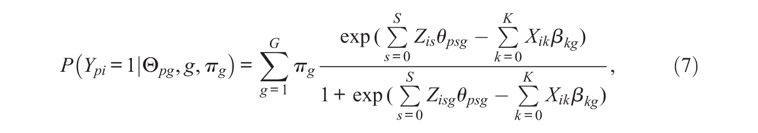
P (Y_{p i} = 1 | Θ_{p g}, g, π_{g}) = \sum_{g = 1}^{G} π_{g} \frac{exp (\sum_{s = 0}^{S} Z_{i s} θ_{p s g} - \sum_{k = 0}^{K} X_{i k} β_{k g})}{1 + exp (\sum_{s = 0}^{S} Z_{i s g} θ_{p s g} - \sum_{k = 0}^{K} X_{i k} β_{k g})},

where g and π_g represent the class membership and mixing proportions, respectively, as in the MixLLTM. Similar to the MixLLTM, the RWLLTM is assumed for each latent class in the MixRWLLTM. However, unlike the MixLLTM, in each class, as presented in Equation 7, there are multiple random effects: the random intercept θ_p_0g and the random coefficients of item property θ_psg, s = 1, . . . , S. In detail, while the random intercept θ_p_0g indicates the general propensity of person p in class g, the random coefficient θ_psg represents the degree to which item property s affects the item difficulties of person p in class g. In other words, these are the person- and class-specific variables.

Therefore, in the MixRWLLTM, the classes are characterized by the fixed coefficients of item property β_kg and the random effects Θ_pg = (θ_p_0g, θ_p_1g, . . . , θ_pSg)′, which follow a multivariate normal distribution with class-specific means and variance-covariance matrix. For example, in the case of incorporating just one random coefficient θ_p_1g in addition to the random intercept θ_p_0g, the Z matrix is composed of the first two columns of the X matrix. The random effects of person p within latent class g, Θ_pg = (θ_p_0g, θ_p_1g)′, are assumed to follow a bivariate normal distribution as

Θ_{pg} = [\begin{matrix} θ_{p 0 g} \\ θ_{p 1 g} \end{matrix}] ~ MV N_{2} ([\begin{matrix} μ_{0 g} \\ μ_{1 g} \end{matrix}], [\begin{matrix} σ_{0 g}^{2} & σ_{01 g} \\ σ_{01 g} & σ_{1 g}^{2} \end{matrix}]),

where μ_0g and μ_1g indicate the class-specific mean of the random intercept and random coefficient, respectively, $σ_{0 g}^{2}$ and $σ_{1 g}^{2}$ are the class-specific variance of the random intercept and random coefficient, respectively, and σ_01g is the class-specific covariance of the two random effects.

We follow the parameterization by Rijmen and De Boeck (2002), in which the fixed effects represent the means of the intercept or the item property difficulties, and the random effects are considered the deviations from these means (the fixed effects). For instance, in the above example, where there is one random coefficient, the difficulty of the first item property corresponds to β_1g−θ_p_1g, and β_1g and θ_p_1g represent the mean (fixed) difficulty of the first item property and person-specific deviation from the mean difficulty, respectively. In other words, the fixed coefficients β_kg, k = 0, 1, . . . , K, indicate the fixed effects or the means of the random effects in latent class g, and hence the means of the random intercept and coefficients are defined as zero by model specifications, such as μ_0g = μ_1g = 0 in Equation 8.

Estimation

Bayesian estimation using MCMC was implemented in the WinBUGS 1.4.3 software (Lunn et al., 2000) to estimate the parameters of the MixRWLLTM and MixLLTM. For this purpose, prior distributions must be specified for all parameters, which include the person-specific ability with class-specific mean and variance, class-specific item property coefficients, group membership, and mixture probabilities. Although each parameter can have a number of different prior distributions, this study limits its scope to the simple and straightforward commonly used ones, such as the conjugate priors. This means that the posterior distribution belongs to the same family as the prior distributions. More specifically, assuming a normal distribution is standard practice for the ability and item parameters, and the conjugate prior for the variance of the normal distribution is the inverse-gamma distribution. It is reasonable to assume that, given the mixture probabilities, each individual’s group membership follows a multinomial distribution, and one of the conjugate priors for the mixture probabilities is the Dirichlet distribution (Cho, Cohen, & Kim, 2013; Cohen & Bolt, 2005; Gelman, Carlin, Stern, & Rubin, 2004).

Consequently, the following prior and hyper-prior distributions were used to estimate the MixLLTM in the present study:

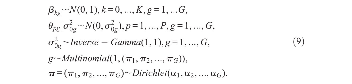
\begin{array}{l} β_{k g} \sim N (0, 1), k = 0, \dots, K, g = 1, \dots G, \\ θ_{p g} | σ_{0 g}^{2} \sim N (0, σ_{0 g}^{2}), p = 1, …, P, g = 1, \dots, G, \\ σ_{0 g}^{2} \sim I n v e r s e - G a m m a (1, 1), g = 1, \dots, G, \\ g \sim M u l t i n o m i a l (1, (π_{1}, π_{2},…, π_{G})), \\ π = (π_{1}, π_{2},…, π_{G}) \sim D i r i c h l e t (α_{1}, α_{2},…, α_{G}) . \end{array}

By model specification, the means of the ability distributions were treated as zero for every class. Mildly informative prior distributions for item property coefficients β_kg and variance of ability $σ_{0 g}^{2}$ were used, and for mixture probabilities, a noninformative Dirichlet prior with α_g = 0.5 was specified (Bolt et al., 2001; Cho et al., 2013; Cohen & Bolt, 2005). Therefore, the posterior distribution can be derived from

\begin{matrix} P (θ_{pg}, σ_{0 g}^{2}, β_{kg}, g, π_{g} | Y) \propto \\ P (Y | θ_{pg}, σ_{0 g}^{2}, β_{kg}, g, π_{g}) P (θ_{pg} | σ_{0 g}^{2}) P (σ_{0 g}^{2}) P (β_{kg}) P (g | π_{g}) P (π_{g}) . \end{matrix}

Considering their distributional assumptions, the only difference between the MixLLTM and MixRWLLTM is the latent ability Θ_pg that includes θ_p_0g and θ_psg. For this variable, we assumed a multivariate normal distribution with mean zero and a variance-covariance matrix ∑_g for each class (as assumed in the RWLLTM). An inverse-Wishart distribution, which is a conjugate prior of the variance and covariance of the multivariate normal distribution, was specified for ∑_g (Gelman et al., 2004). Accordingly, the prior and hyper-prior distributions of ability in the MixRWLLTM were as follows:

\begin{matrix} Θ_{pg} | Σ_{g} ~ MVN (0, Σ_{g}), p = 1, . . ., P, g = 1, . . ., G, \\ Σ_{g} ~ Inverse - Wishart (R_{θ}, r), g = 1, . . ., G, \end{matrix}

where R_θ and r represent the scale matrix and degree of freedom of the inverse-Wishart distribution. For parameters other than the ability, the same prior distributions as the MixLLTM were assumed. The posterior distribution of the MixRWLLTM is derived from

\begin{matrix} P (Θ_{pg}, Σ_{g}, β_{kg}, g, π_{g} | Y) \propto \\ P (Y | Θ_{pg}, Σ_{g}, β_{kg}, g, π_{g}) P (Θ_{pg} | Σ_{g}) P (Σ_{g}) P (β_{kg}) P (g | π_{g}) P (π_{g}) . \end{matrix}

Empirical Data Study

Data Source

Verbal aggression data (Vansteelandt, 2000), previously analyzed by De Boeck (2008) and by Ip, Smits, and De Boeck (2009), were selected to illustrate how the proposed model can be applied to real data (the data can be downloaded from http://bearcenter.berkeley.edu/EIRM/). A total of 316 individuals, 243 females and 73 males, responded to 24 items that described verbally aggressive reactions in a frustrating situation. Responses were dichotomized as 0 for “no” and 1 for “perhaps” or “yes.”

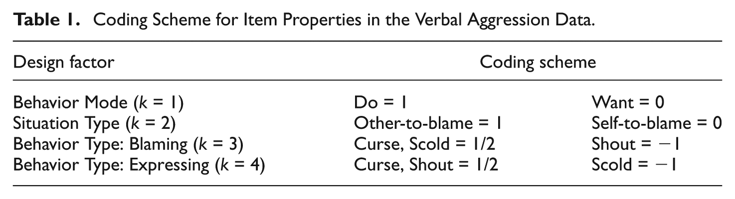
In this example data, the items were developed using four factors that describe a person’s propensity toward verbal aggression. The first design factor reflects the expected tendency that we do not always actually do whatever we want to do. The factor is referred to as the behavior mode, which differentiates between two levels of behavior: wanting to engage in verbal aggression (termed as Want) and actually engaging in verbal aggression (termed as Do). The second design factor is based on the assumption that people display more verbal aggression when others are responsible for discouraging situations. Specifically, this factor, defined as the situation type, contrasts situations in which someone else is to blame (termed as Other-to-blame), such as missing a bus or train because a bus fails to stop, and situations in which the individual is to blame (termed as Self-to-blame) such as a grocery store closing because the person is late. The last two design factors, related to the behavior type, include three levels: Curse, Scold, and Shout. The third and fourth factors are Blaming and Expressing, which deal with the extent to which respondents ascribe blame and express aggression, respectively. Among the three behavior types, cursing and scolding are regarded as blaming and cursing, and shouting as expressive.

For example, the item, “A bus fails to stop for me. I would want to curse” describes factors of want (behavior mode), other-to-blame (situation type), and curse (blaming and expressing). The four design factors are referred to as the item properties, and these item designs enable application of the LLTM and its extended models. The coding scheme for the item properties, which designates the values of the design matrix, is presented in Table 1. In detail, dummy coding was used for the behavior mode and the situation type, in which the want behavior mode and the self-to-blame situation type were the reference categories; and contrast coding was used for the behavior type where the overall mean was the reference category. The item design matrix with the constant item predictor (k = 0) is given in Appendix A.

Table 1.

Coding Scheme for Item Properties in the Verbal Aggression Data.

Design factor	Coding scheme
Behavior Mode (k = 1)	Do = 1	Want = 0
Situation Type (k = 2)	Other-to-blame = 1	Self-to-blame = 0
Behavior Type: Blaming (k = 3)	Curse, Scold = 1/2	Shout = −1
Behavior Type: Expressing (k = 4)	Curse, Shout = 1/2	Scold = −1

Analysis

In the present study, an MCMC algorithm as implemented in WinBUGS was used to extend the LLTM and RWLLTM into mixture models using the verbal aggression data. Three chains with different initial values were specified, and in order to check convergence, time-series plots were monitored. Convergence of the three chains was determined using the $\hat{R}$ index proposed by Gelman and Rubin (1992), with a critical value of 1.01. Depending on these convergence indices and model specifications, the lengths of the iterations were chosen for each model. For example, for the LLTM and RWLLTM, three chains with 3,000 iterations of a burn-in were used in this study followed by 3,000 post-burn-in iterations, and for more complicated models, such as the MixLLTM and MixRWLLTM, 10,000 post-burn-in iterations were made after 10,000 iterations of burn-in.

Furthermore, for ease of interpretation, one random coefficient for the behavior mode (k = 1), θ_p₁, was assumed in addition to the random intercept, θ_p₀, for the random weights models. Thus, in the RWLLTM and MixRWLLTM, S = 1 and Z corresponds to the first two columns of design matrix X . In the mixture models, two latent classes (G = 2) were assumed. In other words, Θ_p and Θ_pg, follow a bivariate normal distribution, and group membership g follows a Bernoulli distribution in the MixLLTM and MixRWLLTM.

Given that the four models, LLTM, MixLLTM, RWLLTM, and MixRWLLTM, considered above are not nested a likelihood ratio (LR) test is not appropriate to compare the relative fit of the models. In the present study, Akaike’s (1974) information criterion (AIC) and Schwarz’s (1978) Bayesian information criterion (BIC) indices were reported, and the BIC was used to determine the better fitting model. Li, Cohen, Kim, and Cho (2009) found that the BIC selects the true data-generating model better than the other methods do, including the AIC and the deviance information criterion (DIC; Spiegelhalter, Best, Carlin, & Van Der Linde, 2002) in mixture dichotomous IRT models using Bayesian estimation. In detail, we followed the method suggested by Li et al. (2009) to define the AIC and BIC for MCMC estimation as

\begin{matrix} AIC = \bar{D (ξ)} + 2 m, \\ BIC = \bar{D (ξ)} + m (\log N), \end{matrix}

where $\bar{D (ξ)}$ is the posterior mean of the deviance, ξ represents all parameters under the model, m refers to the number of estimated parameters, and N indicates the sample size.

Another critical issue in mixture IRT modeling is the label switching problem (Cho et al., 2013; Li et al., 2009). The first type of label switching occurs across iterations within a single MCMC chain, and the second type occurs when the latent classes switch over replications or for different initial values. An occurrence of the first type of label switching results in multiple modes of density for the parameters; thus, the estimated marginal posterior densities were examined in the empirical data analysis in order to detect label switching. In fact, none of the marginal posterior distributions had multiple nodes, which implied that label switching did not occur. The second type of label switching is often observed in simulation studies, as detailed in the simulation study section.

Results

Table 2 summarizes the model fit indices including the AIC and BIC, and the parameter estimates and corresponding standard errors obtained by applying the one-class and two-class LLTM and RWLLTM to the verbal aggression data.

Table 2.

Parameter Estimates and Standard Errors of the One-Class and Two-Class LLTM and RWLLTM.

	One-class LLTM	One-class RWLLTM	Two-class LLTM	Two-class RWLLTM
β₀ (Intercept)	0.311 (0.09)	0.317 (0.10)
β₀₁			0.104 (0.26)	0.295 (0.21)
β₀₂			0.500 (0.18)	0.408 (0.16)
β₁ (Do)	0.670 (0.06)	0.723 (0.08)
β₁₁			1.083 (0.25)	0.802 (0.19)
β₁₂			0.451 (0.18)	0.736 (0.13)
β₂ (Other-to-blame)	−1.023 (0.06)	−1.071 (0.06)
β₂₁			−1.011 (0.16)	−0.912 (0.15)
β₂₂			−1.117 (0.11)	−1.129 (0.12)
β₃ (Blaming)	−1.358 (0.05)	−1.421 (0.52)
β₃₁			−2.575 (0.22)	−2.625 (0.22)
β₃₂			−0.603 (0.12)	−0.608 (0.14)
β₄ (Expressing)	−0.701 (0.05)	−0.734 (0.05)
β₄₁			−1.078 (0.15)	−1.039 (0.13)
β₄₂			−0.487 (0.09)	−0.542 (0.10)
$σ_{0}^{2}$	1.820 (0.18)	2.206 (0.25)
$σ_{01}^{2}$			2.919 (0.91)	3.559 (0.94)
$σ_{02}^{2}$			1.588 (0.43)	1.989 (0.49)
$σ_{1}^{2}$		1.005 (0.18)
$σ_{11}^{2}$				2.044 (0.61)
$σ_{12}^{2}$				0.794 (0.29)
σ ₀₁		−0.424 (0.18)
σ₀₁₁				−1.509 (0.59)
σ₀₁₂				0.025 (0.29)
π ₁			0.477 (0.07)	0.482 (0.07)
AIC	7593.6	7297.5	7196.5	6872.0
BIC	7616.1	7327.6	7245.4	6935.8

Note. The values in parentheses indicate the standard errors associated with the parameter estimates.

First of all, comparisons of the estimated AIC and BIC values suggested that the MixRWLLTM fitted better than the other models did. As presented in Table 2, extensions of the LLTM into the RWLLTM and the MixLLTM yielded better fits than the LLTM did, and the MixLLTM explained the verbal aggression data better than the RWLLTM did. In other words, the two-class LLTM assuming subpopulations described the data more correctly than the one-class RWLLTM allowing a random coefficient of the behavior mode. And most importantly, the two-class RWLLTM, assuming heterogeneous populations that differ in the general propensity of verbal aggression and the effects of the behavior mode property, described the data more correctly than the two-class LLTM. For a more detailed discussion, the fixed and random effect estimates of each model are described below.

Under the LLTM, the estimate of the first design factor ( ${\hat{β}}_{1}$ ) was 0.67, suggesting that the probability of being verbally aggressive decreased when actually doing so compared with wanting to do so. In contrast, the negative estimate of the second design factor ( ${\hat{β}}_{2}$ = −1.023) indicated that examinees became more verbally aggressive in other-to-blame situations than in self-to-blame situations, as we would expect. The estimates of the behavior type (blaming and expressing) were −1.358 and −0.701, respectively, indicating that the blaming aspect of a behavior had greater effects on verbal aggression than the expression aspect. To examine the effects of the three behaviors, coefficients of curse, scold, and shout were calculated, using the coding scheme in Table 1 and the estimates of the third and fourth item properties (see Table 3). Among the three levels of the behavior type, cursing, the combination of blaming and expressing, was the most likely response, and shouting was the least likely response. The variance of the random intercept (θ_p₀) was estimated as ${\hat{σ}}_{0}^{2}$ = 1.82, which represented variability in the general propensity of verbal aggression between persons.

Table 3.

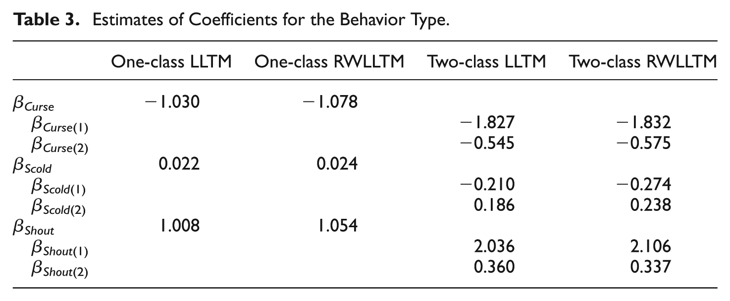
Estimates of Coefficients for the Behavior Type.

	One-class LLTM	One-class RWLLTM	Two-class LLTM	Two-class RWLLTM
β_Curse	−1.030	−1.078
β_Curse₍₁₎			−1.827	−1.832
β_Curse₍₂₎			−0.545	−0.575
β_Scold	0.022	0.024
β_Scold₍₁₎			−0.210	−0.274
β_Scold₍₂₎			0.186	0.238
β_Shout	1.008	1.054
β_Shout₍₁₎			2.036	2.106
β_Shout₍₂₎			0.360	0.337

The third column of Table 2 displays the results of extending the LLTM into the RWLLTM. Comparisons of the estimates of the LLTM and the RWLLTM revealed that similar patterns regarding the fixed effect parameters were found, even though absolute magnitude of the estimates was slightly greater in the RWLLTM. In this model, a random coefficient of the behavior mode (θ_p₁) was included to model individual differences in their tendency to display aggression when the behavior mode changed from wanting to do to actually doing. In detail, while the difference between the two behavior modes was assumed to be constant as β₁ across all examinees in the LLTM, −θ_p₁ was added to the difference for person p in the RWLLTM. As a result, the variance of the random coefficient $(σ_{1}^{2})$ and the covariance of the random intercept and coefficient (σ₁₂) were estimated in the RWLLTM. The results suggested that there was substantial person-to-person variability in the degree of being verbally aggressive for actually doing ( ${\hat{σ}}_{1}^{2}$ = 1.005), and a negative association ( ${\hat{σ}}_{01}$ = −0.424) between the two random effects was found. The meaning of this negative correlation will be detailed below.

As discussed above, mixture extensions of the LLTM and RWLLTM enable us to take advantage of the explanatory aspects of the LLTM and RWLLTM to define characteristics of latent classes. First, the two-class LLTM produced class proportions of approximately 47.8% in Class 1 and 52.2% in Class 2. In this model, the two classes differed in the fixed effects of the item properties and their general propensity of verbal aggression (random intercept). In general, the patterns of the estimated difficulties of the item properties in each class were similar to those in the LLTM. For instance, in the two classes, the probability of being verbally aggressive decreased when going from wanting to do to actually doing, and they were more likely to be aggressive in other-to-blame situations than in self-to-blame situations. However, in Class 1, the coefficient of the behavior mode was much greater, and the coefficients related to the behavior type were smaller than those in Class 2. In other words, compared to Class 2, the tendency to take action decreased much more in Class 1. The estimated coefficients of the three behavior types in Table 3 implied that the examinees in Class 1 were more likely to curse and scold, and less likely to shout than those in Class 2. The variance estimate of the random intercept in Class 1 ( ${\hat{σ}}_{01}^{2}$ = 2.919) was greater than that of Class 2 ( ${\hat{σ}}_{02}^{2}$ = 1.588), which suggested that there was more variability in the general propensity in Class 1 than in Class 2.

As in the MixLLTM, two latent classes of almost equal class size (48.2% in Class 1 and 51.8% in Class 2) were detected in the two-class RWLLTM. Compared to the one-class RWLLTM, the MixRWLLTM found two classes that differed in the fixed coefficients related to the behavior type. In Class 1, ${\hat{β}}_{3}$ and ${\hat{β}}_{4}$ were much smaller than those in Class 2, which resulted in a tendency to curse and scold easily, but to hardly shout in Class 1, compared to people in Class 2. This feature was also found in the classes estimated in the two-class LLTM. However, in the MixRWLLTM, the fixed effects of the behavior mode were not significantly different in the two classes ( ${\hat{β}}_{11}$ = 0.802 and ${\hat{β}}_{12}$ = 0.763). Note that the difference between the want behavior mode and the do behavior mode in Class 1 was a lot greater than in Class 2 in the MixLLTM ( ${\hat{β}}_{11}$ = 1.803 and ${\hat{β}}_{12}$ = 0.451). In other words, after allowing individual differences in the effect of the behavior mode in the MixRWLLTM, the difference between the two classes in the fixed effect of the behavior mode disappeared.

More interestingly, the MixRWLLTM found that the two classes did differ in a meaningful way with respect to the random effects. In this model, by introducing a person-specific random effect of the behavior mode, the latent trait was assumed to follow a mixture of two bivariate normal distributions. In Class 1, the estimated variance of the intercept ( ${\hat{σ}}_{01}^{2}$ = 3.559) was greater than the variance of the random coefficient of the behavior mode ( ${\hat{σ}}_{11}^{2}$ = 2.044), and there was a negative association between the two random effects ( ${\hat{σ}}_{011}$ = −1.509). The estimated correlation was −0.567, which was significantly different from zero at the 5% level. In Class 2, the variance estimate of the intercept ( ${\hat{σ}}_{02}^{2}$ = 2.044) was greater than the variance estimate of the random coefficient ( ${\hat{σ}}_{12}^{2}$ = 0.794), as in Class 1. However, unlike Class 1, the estimated covariance of the two random effects was a small positive value in Class 2 ( ${\hat{σ}}_{012}$ = 0.025). The estimated correlation 0.02 was not significantly different from zero at the 5% level. In sum, there was more person-to-person variability in the random intercept than in the random coefficient in the two classes, and the two random effects of Class 1 were more heterogeneous than those of Class 2.

Moreover, the estimated correlations between the two random effects delineated the difference between the two classes more clearly. Specifically, the negative correlation in Class 1 meant that people who had a higher propensity toward verbal aggression appeared to have a smaller random coefficient of the behavior mode. Given that the coefficient of the behavior mode for person p, represented as β₁−θ_p₁, indicates the difference in the probability of wanting to take verbally aggressive action and of actually doing, this result implied that, as the general propensity of verbal aggression (θ_p₀) increased, the random coefficient (θ_p₁) decreased; thus the difference between wanting and doing increased. However, in Class 2, the general propensity of verbal aggression and the random coefficient of the behavior mode were virtually independent of each other. The estimates of the latent variables related to the general propensity and the coefficient of the behavior mode for each class in the MixRWLLTM are presented in Figure 1.

Figure 1.

Diagram of estimated Θ_pg by each latent dimension.

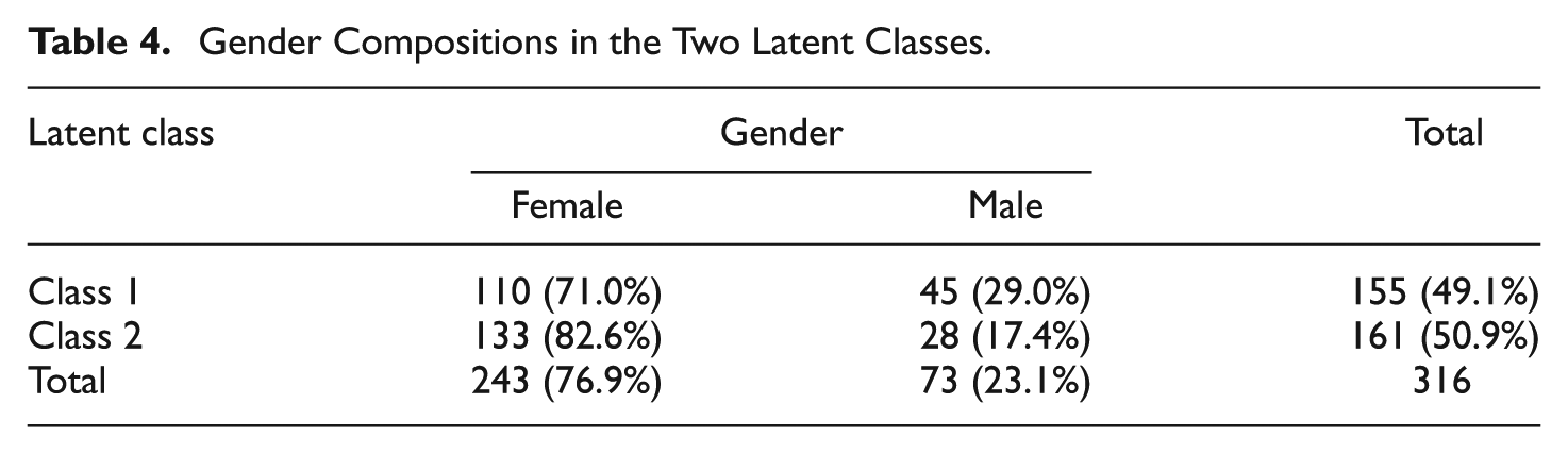
In addition to estimates of the item parameters, the variances of the latent ability distributions, and the mixing proportions, examinees in mixture item response models are also characterized by a parameter that indicates each examinee’s latent group membership g. In the two-class RWLLTM, the estimated mixing proportions classified 155 (110 females and 45 males) examinees into Class 1 and 161 (133 females and 28 males) examinees into Class 2 (see Table 4). In the total sample, the proportions of females and males were 76.9% and 23.1%, respectively, while the proportions in Class 1 were 71% and 29%, respectively, and the proportions in Class 2 were 82.6% and 17.4%. There were more males in Class 1 and more females in Class 2 than in the total sample. The chi-square test of independence indicated that gender was associated with class membership (p < 0.05), although the correlation between gender and class membership was weak (ρ = 0.138).

Table 4.

Gender Compositions in the Two Latent Classes.

Latent class	Gender		Total
	Female	Male
Class 1	110 (71.0%)	45 (29.0%)	155 (49.1%)
Class 2	133 (82.6%)	28 (17.4%)	161 (50.9%)
Total	243 (76.9%)	73 (23.1%)	316

Simulation Study

Data Generation

The simulation design followed the empirical example of the verbal aggression data, as described previously. The data were generated from the two-class RWLLTM, in which 1,000 examinees responded to test items designed using the four item properties, as in the empirical application. The simulation design included two test lengths: 24 items and 48 items. In the 24-item condition, the design matrix used for the verbal aggression data was assumed. In the case of the 48-item condition, the elements of the design matrix for the first 24 items were repeated for the last 24 items.

The structure of the verbal aggression data was kept, and the estimates of the two-class RWLLTM, presented in the fifth column of Table 2, were assumed as the true values in the data generation. In other words, two latent classes, with class size parameters π = (0.482, 0.518), were assumed, and only one coefficient of the first item design factor was treated as random. The data generating model was a two-class and two-dimensional model containing one random intercept and one random coefficient. Thus, the latent traits within a class follow a bivariate normal distribution with class-specific means and variance-covariance matrix. As noted previously, the means of the random effects were constrained to zero in each class. The variance-covariance matrices of the random effects for each class were specified as

Θ_{p 1} \sim M V N_{2} ([\begin{matrix} 0 \\ 0 \end{matrix}], [\begin{matrix} 3.559 & - 1.509 \\ - 1.509 & 1.989 \end{matrix}]), Θ_{p 2} \sim M V N_{2} ([\begin{matrix} 0 \\ 0 \end{matrix}], [\begin{matrix} 2.044 & 0.025 \\ 0.025 & 0.794 \end{matrix}]) .

In addition, the two classes depend on the fixed coefficients of the item properties. The R software (R Core Team, 2013) was used to generate the data and 30 replications were made for each condition of the two test lengths.

Analysis

Once the data were generated, the two-class RWLLTM, was applied using the MCMC algorithm. As implemented in the empirical data application, WinBUGS was run using three chains with 10,000 post-burn-in iterations after discarding 10,000 burn-in iterations. Convergence of the three chains was determined by the Gelman and Rubin (1992) method.

The second type of label switching in mixture item response models, which refers to class switching over replications, was observed in the simulation study described here. For example, if label switching has occurred, Class 1 in one replication corresponds to Class 2 in the true model; thus, labels of the parameter estimates and group membership need to be switched, such as from Class 1 to Class 2. Given that we know the true values of the parameters in the simulation study, the detection of label switching is possible by simply comparing the item parameter estimates and estimated group membership with the generating values (Cho et al., 2013; Li et al., 2009). In this simulation study, the covariance of the random effects, of which true value in Class 1 was negative and larger in absolute value than the one in Class 2, was used to detect label switching.

Results

After adjusting for label switching, the bias and root mean square error (RMSE) of the parameters in each class were assessed, and they are reported in Table 5. In general, the estimated biases were not substantial under the two test length conditions. According to the one-sample t-test, none of these bias estimates was significantly different from zero at the 5% level. These results suggested that the estimates of the generating model were approximately unbiased. The RMSEs in the 48-item condition were slightly smaller than those in the 24-item condition.

Table 5.

Bias and RMSE of Parameters in the Simulation Study.

		P = 1,000, I = 24		P = 1,000, I = 48
	True	Bias	RMSE	True	Bias
Class 1
β₀₁	0.295	0.023	0.076	−0.035	0.079
β₁₁	0.802	−0.024	0.088	0.008	0.076
β₂₁	−0.912	−0.004	0.066	−0.012	0.037
β₃₁	−2.625	−0.001	0.080	−0.010	0.031
β₄₁	−1.039	0.015	0.044	−0.001	0.029
$σ_{01}^{2}$	3.559	0.006	0.083	−0.007	0.079
$σ_{11}^{2}$	2.044	0.003	0.096	−0.013	0.087
σ₀₁₁	−1.509	−0.019	0.090	−0.002	0.079
π₁	0.482	0.015	0.029	0.021	0.027
Class 2
β₀₂	0.408	−0.027	0.086	0.015	0.076
β₁₂	0.736	0.006	0.068	−0.004	0.052
β₂₂	−1.129	0.017	0.044	0.008	0.034
β₃₂	−0.608	−0.007	0.043	−0.005	0.033
β₄₂	−0.542	−0.013	0.034	−0.005	0.025
$σ_{02}^{2}$	1.989	−0.001	0.097	0.021	0.074
$σ_{12}^{2}$	0.794	0.016	0.091	0.001	0.080
σ₀₁₂	0.025	0.005	0.083	−0.015	0.083

In addition, recovery of group membership was investigated by comparing the estimated latent group membership with the generating one, and the percentage of correct identification was evaluated in each replication. The averages of the percentage of correct identification across 30 replications were 86.69% and 93.8% for the 24- and 48-item conditions, respectively, indicating that recovery of group membership increased as the test length increased.

Discussion and Conclusions

In this study, the MixRWLLTM was developed to find multiple subgroups of examinees and to interpret the meaning of latent classes. The existence of subgroups is identified using latent class analysis or mixture item response modeling; however, the meaning of latent classes can be specified only after estimated class-specific parameters, such as item difficulties and distributions of the latent variables, are interpreted and compared across latent classes. This study showed that the MixRWLLTM can contribute to a better understanding of characteristics of latent classes, by incorporating the explanatory aspect of the LLTM and the individual differences of examinees captured by the RWLLTM.

For instance, in the MixRWLLTM, the fixed class-specific coefficients of the item properties describe how people within each class would respond differently on items related to the item properties. Because the item property coefficients represent the fixed effects, interpretations based on these parameters are assumed to be the same across individuals within the same class, and therefore, describe overall characteristics of latent classes.

Moreover, the MixRWLLTM allows individual differences in the effects of the item features, as in the RWLLTM. Within each class of the MixRWLLTM, each individual has person-specific random effects in the general latent variable the test items intend to measure and in the coefficients of certain item features. Therefore, individual differences in these multidimensional aspects and relations across multiple dimensions can be used to disclose key characteristics of latent classes. Furthermore, given that in the MixLLTM the meaning of latent classes is determined based mainly on the fixed coefficients of the item properties, we expect that the MixRWLLTM provides a more comprehensive understanding of how latent classes are defined and why people across classes respond or behave differently.

The illustrative example, using the verbal aggression data, showed that the MixRWLLTM yielded much better agreement with the data than the LLTM, RWLLTM, and MixLLTM did. Additionally, in order to compare performance of the MixRWLLTM to the mixture Rasch model, the verbal aggression data were also analyzed using the two-class Rasch model. In the mixture Rasch model, the item design features in the verbal aggression data were not considered and the difficulties of the 24 items were estimated for the two classes. The estimated values of the AIC and BIC of the mixture Rasch model supported a better fitting of the MixRWLLTM to the data.² In other words, by taking into account the design features of items, the MixRWLLTM provided more correct description of the data.

In addition to improving goodness of fit, the MixRWLLTM revealed an interesting difference across latent classes that was not detected by the other approaches. The MixRWLLTM identified two distinct classes that differed considerably in relations between the general propensity toward verbal aggression and the random effect related to the behavior mode. In general, the results indicated that people in the two classes were reluctant to actually take verbally aggressive action compared to just wanting to do so, based on the class-specific fixed coefficients of the behavior mode. However, in one class, people whose general propensity toward verbal aggression was higher displayed a greater difference between their tendency to want and to actually do; thus, they were more reluctant to take action. In sum, the empirical data study suggested that interpretations of latent classes in the MixRWLLTM can be improved by considering the multidimensional random effects of respondents, and more specifically, by using their general latent trait and person-specific effect of an item feature. In this regard, cognitive theories or features of the items, which direct the instrument development in the LLTM, also enrich interpretations of classes in the mixture extensions of the LLTM.

The simulation study indicated that Bayesian estimation using WinBUGS appeared to recover the parameters and group membership of the MixRWLLTM fairly well. By increasing the number of test items, recovery of group membership of the MixRWLLTM increased.

Overall, the results from the empirical and simulation studies suggested that the MixRWLLTM was able to identify the latent classes of examinees and that the item design properties could play a crucial role in an improved understanding of characteristics of latent classes. There are also some possible extensions of the current model. Here, because the primary goal of the study was to extend the RWLLTM into the mixture model, we limited ourselves to a simple model by classifying examinees into two classes. However, it is possible to introduce more than two latent classes (e.g., Cho et al., 2013; Frederickx, Tuerlinckx, De Boeck, & Magis, 2010). The WinBUGS code given in the Appendix B can be easily generalized to deal with more than two classes. Likewise, more random coefficients of the item properties can be included.

One concern in applications using mixture item response models is that they may not always detect the true latent classes, but yield spurious latent classes; for example, Alexeev, Templin, and Cohen (2011) showed that fitting the mixture Rasch model to data generated by the 2PL model could produce false classes. In a supplementary simulation, to examine whether the classes detected via the MixRWLLTM were spurious or not, we generated data from the one-class RWLLTM, and the one- and two-class RWLLTMs were fitted to the data. Across 15 replications, the estimated BIC values were consistently lower for the one-class RWLLTM, which suggested that spurious classes were not found. However, when the one- and two-class LLTMs were fitted to the data, the two-class LLTM yielded a better fit than the one-class LLTM across all the replications. Consequently, according to these additional simulations, the MixRWLLTM developed in the present study did not produce latent classes when indeed there were none but the MixLLTM did. Thus, when the multidimensional structure of the random effects is not modeled appropriately (i.e., fitting the MixLLTM to the data generated by the RWLLTM), spurious classes can be produced. Even though these simulations have not shown a problem regarding false classes for the MixRWLLTM, further studies should be carried out to investigate the possibility of detecting spurious latent classes in the context of multidimensional IRT models.

In the present study, we have successfully applied the Bayesian approach to estimate the MixRWLLTM, using conjugate and mildly informative prior distributions in order to make the fitting procedures more stable (Bolt et al., 2001, 2002; Cho & Cohen, 2010). However, given that the specification of the prior distributions could have substantial impacts on estimation (Gelman, 2006), it is worth investigating more deeply the use of different prior distributions. In order to examine the sensitivity to the prior distributions, less informative priors on the item property coefficients such as N(0, 10) and N(0, 100) were employed in the empirical data analysis. We found that the use of less informative priors yielded estimates only slightly different from the ones using the mildly informative prior, which suggested that the results of the present study were robust to the specification of the prior distributions.

Finally, the MCMC procedures implemented in WinBUGS required substantial computing time for convergence, which is not uncommon in MCMC estimation. To enhance the practical use of the proposed model, other software that handles multidimensional mixture models for discrete data (e.g., LatentGold; Vermunt & Magidson, 2005) might be considered for future studies.

Footnotes

Appendix A

Appendix B

Declaration of Conflicting Interests

The author(s) declared no potential conflicts of interest with respect to the research, authorship, and/or publication of this article.

Funding

The author(s) received no financial support for the research, authorship, and/or publication of this article.

Notes

References

Adams

R. J.

Wilson

Wang

(1997). The multidimensional random coefficients multinomial logit model. Applied Psychological Measurement, 21(1), 1-23.

Adams

R. J.

Wilson

(1997). Multilevel item response models: An approach to errors in variables regression. Journal of Educational and Behavioral Statistics, 22(1), 47-76.

Akaike

(1974). A new look at the statistical model identification. IEEE Transactions on Automatic Control, 19, 716-723.

Alexeev

Templin

Cohen

A. S.

(2011). Spurious latent classes in the mixture Rasch model. Journal of Educational Measurement, 48, 313-332.

Bolt

D. M.

Cohen

A. S.

Wollack

J. A.

(2001). A mixture item response model for multiple-choice data. Journal of Educational and Behavioral Statistics, 26, 381-409.

Bolt

D. M.

Cohen

A. S.

Wollack

J. A.

(2002). Item parameter estimation under conditions of test speededness: Application of a mixture Rasch model with ordinal constraints. Journal of Educational Measurement, 39, 331-348.

Cho

S.-J.

Cohen

A. S.

(2010). A multilevel mixture IRT model with an application to DIF. Journal of Educational and Behavioral Statistics, 35, 336-370.

Cho

S.-J.

Cohen

A. S.

Kim

S.-H.

(2013). Markov chain Monte Carlo estimation of a mixture item response theory model. Journal of Statistical Computation and Simulation, 38, 278-306.

Cohen

A. S.

Bolt

D. M.

(2005). A mixture model analysis of differential item functioning. Journal of Educational Measurement, 42, 133-148.

10.

De Boeck

(2008). Random item IRT models. Psychometrika, 73, 533-559.

11.

De Boeck

Cho

S.-J.

Wilson

(2011). Explanatory secondary dimension modeling of latent differential item functioning. Applied Psychological Measurement, 35, 583-603.

12.

De Boeck

Wilson

(Eds.). (2004). Explanatory item response models: A generalized linear and nonlinear approach. New York, NY: Springer.

13.

De Boeck

Wilson

Acton

G. S.

(2005). A conceptual and psychometric framework for distinguishing categories and dimensions. Psychological Review, 112, 129-158.

14.

Draney

Wilson

Gluck

Spiel

(2008). Mixture models in a developmental context. In Hancock

Samuelsen

(Eds.), Advances in latent variable mixture models (pp. 199-216). New York, NY: Information Age.

15.

Fischer

G. H.

(1973). The linear logistic test model as an instrument in educational research. Acta Psychologica, 37, 359-374.

16.

Frederickx

Tuerlinckx

De Boeck

Magis

(2010). RIM: A random item mixture model to detect differential item functioning. Journal of Educational Measurement, 47, 432-457.

17.

Gelman

(2006). Prior distributions for variance parameters in hierarchical models. Bayesian Analysis, 1, 515-534.

18.

Gelman

Carlin

J. B.

Stern

H. S.

Rubin

D. B.

(2004). Bayesian data analysis. Boca Raton, FL: Chapman & Hall/CRC.

19.

Gelman

Rubin

D. B.

(1992). Inference from iterative simulation using multiple sequences. Statistical Science, 7, 457-472.

20.

E. H.

Smits

D. J. M.

De Boeck

(2009). Locally dependent linear logistic test model with person covariates. Applied Psychological Measurement, 33, 555-569.

21.

Cohen

A. S.

Kim

S.-H.

Cho

S.-J.

(2009). Model selection methods for mixture dichotomous IRT models. Applied Psychological Measurement, 33, 353-373.

22.

Lunn

D. J.

Thomas

Best

Spiegelhalter

(2000). WinBUGS—A Bayesian modelling framework: Concepts, structure, and extensibility. Statistics and Computing, 10, 325-337.

23.

Meyer

J. P.

(2010). A mixture Rasch model with item response time components. Applied Psychological Measurement, 34, 521-538.

24.

Mislevy

R. J.

Verhelst

(1990). Modeling item responses when different subjects employ different solution strategies. Psychometrika, 55, 195-215.

25.

R Core Team. (2013). R: A language and environment for statistical computing. Vienna, Austria: R Foundation for Statistical Computing. Retrieved from http://www.R-project.org

26.

Rijmen

De Boeck

(2002). The random weights linear logistic test model. Applied Psychological Measurement, 26, 271-285.

27.

Rost

(1990). Rasch models in latent classes: An integration of two approaches to item analysis. Applied Psychological Measurement, 14, 271-282.

28.

Schwarz

(1978). Estimating the dimension of a model. Annals of Statistics, 6, 461-464.

29.

Spiegelhalter

D. J.

Best

N. G.

Carlin

B. P.

Van Der Linde

(2002). Bayesian measures of model complexity and fit. Journal of the Royal Statistical Society: Series B. Statistical Methodology, 64, 583-639.

30.

Vansteelandt

(2000). Formal models for contextualized personality psychology (Unpublished doctoral dissertation). K.U. Leuven, Belgium.

31.

Vermunt

J. K.

Magidson

(2005). Latent GOLD 4.0 user’s guide. Belmont, MA: Statistical Innovations.

32.

Wilson

(1989). Saltus: A psychometric model of discontinuity in cognitive development. Psychological Bulletin, 105, 276-289.