Detecting Test Tampering Using Item Response Theory

Abstract

Test tampering, especially on tests for educational accountability, is an unfortunate reality, necessitating that the state (or its testing vendor) perform data forensic analyses, such as erasure analyses, to look for signs of possible malfeasance. Few statistical approaches exist for detecting fraudulent erasures, and those that do largely do not lend themselves to making probabilistic statements about the likelihood of the observations. In this article, a new erasure detection index, EDI, is developed, which uses item response theory to compare the number of observed wrong-to-right erasures to the number expected due to chance, conditional on the examinee’s ability-level and number of erased items. A simulation study is presented to evaluate the Type I error rate and power of EDI under various types of fraudulent and benign erasures. Results show that EDI with a correction for continuity yields Type I error rates that are less than or equal to nominal levels for every condition studied, and has high power to detect even small amounts of tampering among the students for whom tampering is most likely.

Keywords

test tampering erasure detection wrong-to-right erasures teacher cheating ability purification

The cheating scandal in the Atlanta Public Schools (see Kingston, 2013) brought the issue of test tampering into the national spotlight. Although Atlanta was not the first instance in which teachers were found to have engaged in changing students’ answers after tests were complete (Asimov & Wallack, 2007; McGraw & Woo, 1988), it has demonstrated the severity of the problem like no previous cheating scandal, and has sent a clear signal to districts and states that they should be actively looking for signs of teacher/administrator tampering.

Test tampering is most commonly associated with paper-based testing, where educators may change student answers after the tests are complete. It is for this reason that both Smarter Balanced and PARCC assessments will be predominantly computer-based, and many other educational accountability programs are moving toward computer-based tests. However, lack of computer capacity is causing the transition from paper-to-computer delivery to happen slowly for many states (Camara, personal communication, September 19, 2014). Accountability programs such as ACT, Iowa Assessments, and the New York Regents exam are all largely or exclusively paper-based and are anticipating continuing with that platform as the primary mode of delivery for the foreseeable future.

However, depending on the administrative conditions, test tampering may also be possible in the computer-based testing environment. Tests that are administered with scheduled breaks after which students can resume the test are also susceptible to tampering by educators, as are any tests for which students are instructed not to submit their answers immediately on finishing.

Detection of test tampering is usually approached from one of two angles. The first of these is with models that focus on detecting unusually large gains (Skorupski & Egan, 2012; Wollack & Maynes, 2011). Within the school context, approaches looking at gains detect not only tampering, but also illegal coaching. One of the inherent challenges in approaches focused on gains is that the goal of education is to produce learning gains. Therefore, distinguishing between gains due to learning and gains due to cheating becomes critical. Unusual gains that are achieved through test tampering are often accompanied by large numbers of erasures, particularly wrong-to-right erasures (WTR). Therefore, the second approach to detecting test tampering is through analyzing secondary light marks on answer sheets that are indicative of erasures. There are multiple reasons that an individual student may produce many erasures, but an unusually high number of erasures or WTR erasures for an entire class is very difficult to attribute to anything other than test tampering. For this reason, erasure analysis is often regarded as a useful approach for detecting test tampering.

Erasure detection is a very new science. Existing approaches to detection have overwhelmingly been empirical, creating a distribution of the observed number of erasures (or perhaps WTR erasures) or developing a statistical model that fits empirical data well. An examinee or a group is identified as anomalous if they fall in the upper tail of the distribution or produce a number of WTR erasures that are a predetermined number of standard deviations above the mean (Bishop, Liassou, Bulut, Seo, & Bishop, 2011; Maynes, 2013; Primoli, Liassou, Bishop, & Nhouyvanisvong, 2011). Such empirical approaches have been executed successfully in other forms of cheating detection, such as answer copying or similarity (Allen, 2012; Hanson, Harris, & Brennan, 1987). However, in answer copying contexts, it is customary to build the baseline empirical sampling distribution by pairing students from different testing centers for whom copying was impossible. Consequently, the baseline distribution represents a null distribution. In the erasure context, however, no clear mechanism exists to develop a distribution based on null cases only; hence, the methodologies create sampling distributions that may be, to some extent, contaminated by fraudulent erasures. As a result, it is not possible using these methodologies to have a clear understanding of the error rates (Type I or Type II) associated with the statistical findings. Similarly, empirical approaches, such as have been done, do not allow for accurate probabilistic statements of the likelihood of the result, and produce sample-dependent estimates of the extremity of results.

van der Linden and Jeon (2012) modeled erasure behavior by assuming that all final answers were reached through a two-stage process in which, in Stage 1, every item (i = 1, . . ., n) is answered, and in Stage 2, every item is revisited and the answer is either changed (producing an erasure) or retained (not producing an erasure). Using item response theory, and assuming that examinee j’s θ_j (j = 1, . . ., N) remains constant throughout the test, item parameters for a two-parameter model are fit to the N× 2n data set, allowing the initial and final items to be separately calibrated. van der Linden and Jeon derived the models for the four conditional probabilities of final responses (e.g., final answers are correct or incorrect conditioned on the initial answers being correct or incorrect). The probability of a final correct answer conditional on an incorrect initial response follows as the probability of a WTR erasure. Using this model, the van der Linden and Jeon approach uses the generalized binomial to derive, for each individual, the exact probability distribution of the number of WTR erasures conditional on the specific set of items that were initially answered incorrectly. Under this approach, examinees with observed WTR scores that are sufficiently improbable are flagged as anomalous.

In this study, we adopt an approach similar to that of van der Linden and Jeon in that we use item response theory to model erasure data, and subsequently develop an index that evaluates the number of WTR erasures against the number expected under the model. This model is evaluated through simulation, as well as analytically, and data on the Type I error rate and power are provided. We conclude with some thoughts about the implications for practitioners.

Development of a New Erasure Detection Index

As mentioned previously, erased items are not indicative of tampering; however, tampered questions will result in erasures. Consequently, the validity of responses to erased items should be approached with some suspicion, particularly if there are many such items on an exam. Furthermore, if trait estimation for examinee j includes tampered items, ${\hat{θ}}_{j}$ will be spuriously large. As a result, the method here estimates θ_j values for all examinees using only the subset of items for which no evidence of tampering exists (i.e., items that were not erased). That is, if I_E,j is the set of items for which examinee j produced erasures, ${\hat{θ}}_{j}$ is estimated here including only those items such that $i \notin I_{E, j}$ . Therefore, we will use ${\hat{θ}}_{j [i \notin I_{E, j}]}$ to accentuate the fact that trait levels are estimated using only nonerased items.

The assumption in cases of test tampering is that answers will be changed from incorrect to correct, thereby producing an artificially high number correct score. Hence, our interest is in comparing the observed number correct score across erased items to the expected number correct score across those same items.

The observed score on erased items, $X_{j, I_{E, j}}$ , is computed as follows:

X_{j, I_{E, j}} = \sum_{i \in I_{E, j}} x_{ij},

where x_ij is the right/wrong score for examinee j on item i. This quantity has been shown to follow a generalized binomial distribution (van der Linden & Jeon, 2012; van der Linden & Sotaridona, 2006). However, for purposes of this study, $X_{j, I_{E, j}}$ will be modeled with a normal approximation to the binomial. Again, using ${\hat{θ}}_{j [i \notin I_{E, j}]}$ and estimates of the item parameters, the expected number correct score, $E (X_{j, I_{E, j}}),$ is computed as follows:

E (X_{j, I_{E, j}}) = \sum_{i \in I_{E, j}} P (x_{ij} = 1) .

Any item response model appropriate for the data may be used to estimate P(x_ij = 1).

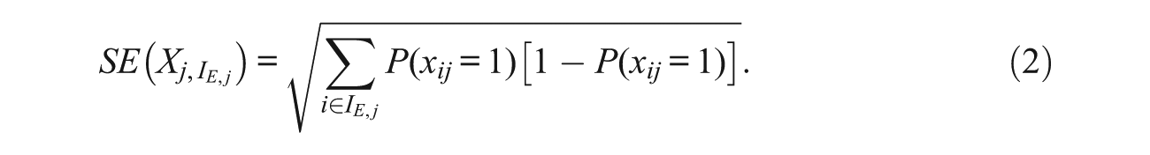
The appropriate standard error for $X_{j, I_{E, j}}$ is given by

SE (X_{j, I_{E, j}}) = \sqrt{\sum_{i \in I_{E, j}} P (x_{ij} = 1) [1 - P (x_{ij} = 1)]} .

The erasure detection index (EDI) used to determine whether the number of WTR erasures exceeds that expected due to chance is

EDI = \frac{X_{j, I_{E, j}} - E (X_{j, I_{E, j}}) + C}{SE (X_{j, I_{E, j}})} .

Previous research has found that indexes of this structure (e.g., the ω statistic for answer copying detection [Wollack, 1997]) have somewhat inflated false positive rates for low ability examinees when tests are short (van der Linden & Sotaridona, 2006). Because the number of erased items is likely to be a subset of all items, it is expected that, even in cases where tampering occurred, the maximum value of $X_{j, I_{E, j}}$ will be relatively small, so EDI should behave in a manner consistent with how other similar indexes perform on short tests. It is, therefore, reasonable to assume that application of a correction for continuity could help to better control the false positive error rate in all conditions. Hence, the quantity C in the numerator represents a correction for continuity. The extent to which such a correction improves the false positive rate of the EDI will be examined as part of this study.

Simulating Erasures

Two different types of erasures were simulated—benign erasures, in which examinees legitimately erased and changed their answers on reconsideration of the item choices, and fraudulent erasures, in which a test administrator (e.g., teacher, proctor, principal, etc.) erased and changed students’ answers after the test was over. The data set analyzed was simulated to simultaneously include both types of erasures, including some students whose item response vectors consisted of a combination of benign and fraudulent erasures, so as to be consistent with the situation in practice, when all types of erasures may be embedded in a data set.

As a first step in the simulation, responses were generated for 250,000 examinees on a 50-item 5-alternative multiple-choice test using the nominal response model (NRM; Bock, 1972). The distribution of examinee ability was assumed to be normal (e.g., θ ~ N(0, 1)). NRM item parameter estimates from an English language usage test administered to nearly 25,000 college freshmen were treated as the generating parameters.

Next, benign erasures were simulated. According to the research, erasures on state accountability exams are not common. Primoli et al. (2011) conducted a comprehensive study of erasure rates in which they analyzed 3 years’ worth of data from 45 tests in eight subject areas in nine grades as part of four different state testing programs. On average, they found the distribution of erasures to be heavily positively skewed. Examinees produced erasures on approximately 2% of the items. Mroch, Lu, Huang, and Harris (2012) found erasures to be even less prevalent, thereby supporting the assertion that erasures of any sort are generally uncommon.

In this study, three different types of benign erasures were simulated. Random erasures refer to situations in which a student either accidently bubbles in the wrong answer on the answer sheet, identifies it immediately, and changes it to the intended answer, or the case in which a student initially answers an item one way, but on reconsideration, changes that answer. Misalignment erasures (sometimes called shift errors) refer to situations in which a student accidently bubbles in the answer to item i in the space on the answer sheet reserved for item i+1 (or i−1), and continues to mark answers for a string of consecutive items in the wrong fields. The erasure comes about when the student finally realizes the mistake, erases the answers to the misaligned items, and marks those same answers again, this time in the correct fields on the answer sheet. String-end erasures refer to the situation in which students find that they are running out of time, so randomly fill in answers to the remaining questions to make sure that no questions are left unanswered. As time permits, the students return to the questions and answer them on merit, erasing and changing the answers, if necessary.

In this study, each simulee was simulated to have Y_j benign erasures. Because misalignment and string-end erasures both would be very rare occurrences, these types of erasures were each simulated for 1,000 students. To facilitate studying the performance of EDI for examinees of different ability levels, examinees were sorted into quintile groups based on θ. For each condition, 200 students within each quintile group were randomly selected to produce misalignment erasures, and another 200 were simulated to produce string-end erasures. The remaining 248,000 students were simulated to have random erasures.

For simulees selected for random erasures, Y_j was generated from a binomial distribution with p = .02 and N = 50 (the number of items). Consequently, on average, examinees had one random erasure and nearly three-quarters of the examinees were simulated to have zero or one benign, random erasure. Under this model, only 6 in 100,000 examinees would have 7 or more random erasures. A graph of the expected benign random erasure distribution is shown in Figure 1.

Figure 1.

Binomial distribution with N = 50 and p = .02 used to simulate the number of benign random erasures per examinee.

After finding the number of random erasures per examinee, for each examinee, Y_j random numbers from U[1,50] were drawn, without replacement, to identify the specific items on which student j produced a random erasure. For each erased item for person j, a second response was generated using the NRM, conditional on the response being different than the original answer. These new responses were taken to be the examinees’ initial responses which were subsequently erased. The originally simulated answers (which allowed simulees to choose any of the response options) were taken as the final answers.

If indicator function I_ijν = 0 when ν equals the final response by person j to item i, initial responses were generated based on probabilities from the conditional NRM shown below

P_{iv} (θ_{j}) = \frac{\exp (Z_{iv} (θ_{j})) \cdot I_{ijv}}{\sum_{k = 1}^{m_{i}} [\exp (Z_{ik} (θ_{j})) \cdot I_{ijk}]},

where m_i denotes the number of alternatives for item i, and Z_iν(θ_j) = ζ_iν+λ_iνθ_j, with ζ_iν and λ_iν being the NRM slope and intercept parameters, respectively, for alternative ν of item i.

Misalignment issues, if undetected for a long time, will produce a rather large number of erasures. Here, we use a binomial distribution with N = 50 and p = .25 to identify the number of misaligned items for simulee j, M_j. Note that M_j provides an upper bound for Y_j, because not all alignment errors will result in erasures. This distribution for M_j, shown in Figure 2, produces rather long sequences of misaligned items. On average, examinees in this condition misalign 12.5 items, and approximately 80% of examinees produce between 9 and 16 misalignments. To identify the location of the first misaligned item, we randomly generated a number from a U[1, 50 −M_j+1]. For each misaligned item, we compared the response indicated for item in position i with the response indicated for item i− 1. If they were different, the response to item i− 1 was taken as the erased response for item i. If the responses to the two items were the same, this suggests that the correctly marked item happened to be marked the same way as the misaligned item, so it would not be identified as an erasure.

Figure 2.

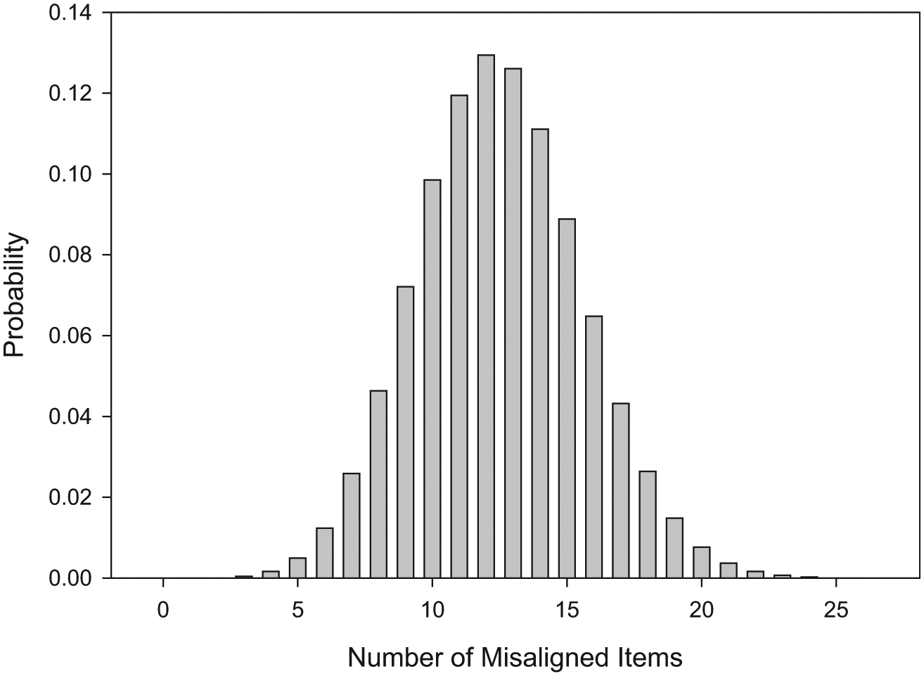
Binomial distribution with N = 50 and p = .25 used to simulate the number of misaligned items.

String-end erasures, like misalignments, have potential to involve long strings of items. In the interest of consistency with the misaligned examinees, string-end erasures were simulated by generating a randomly guessed initial response for the last 12 items on the exam (Items 39-50) such that the probability of selecting each alternative was equal to 0.2. In cases where the randomly selected alternative matches the answer from the final data, the item would not be detected as an erasure.

Fraudulent erasures were simulated on top of the benign erasures, so that simulees with fraudulent erasures likely had benign erasures too. Within each quintile group, a total of 1,000 examinees were randomly selected to be victims of tampering. Two different types of fraudulent erasures were simulated: fixed and variable tampering. In the fixed tampering conditions, a fixed number of items were erased and changed to be correct. Because correctly answered questions would not likely be erased (and even if they were, they would be replaced by bubbling in the same circle), only items that were answered incorrectly originally were candidates to be erased and changed. For each examinee, the incorrectly answered items were all equally likely to be erased and changed to correct. The fixed tampering condition had three levels: 5 items, 10 items, and 15 items. Given the test lengths, it is understood that examinees in the higher quintile groups may not have had enough incorrectly answered items to allow for changing as many items as was required for the condition. In this case, all incorrectly answered items were changed to be correct.

In the variable tampering condition, we simulated a situation in which an administrator changed just enough items to help a student get from not proficient to proficient. Because some simulees are farther from the proficiency cutoff than others, this resulted in different numbers of items being erased for each person. According to Hull (2008), the average percentage of students proficient in math across the United States is approximately 55%. Under the assumption of an underlying normal ability distribution, the 55th percentile corresponds to a θ = −0.126. Given the test characteristic curve associated with the generating item parameters in this study, a θ = −0.126 corresponded to a true score of 26.66. Because 26.66 was not a possible raw score, for purposes of this study, we define as proficient any examinees with scores of 26 or higher.

As in the previous simulation, 1,000 simulees within each quintile group were randomly selected as tampered examinees. Because only students below the 45th percentile were eligible to be selected, no simulees in quintiles 4 or 5, and only the lowest scoring simulees from quintile 3 were selected. The number of erased items per simulee was based not on their number correct score, but on their true score, as it seems more likely to these authors that teachers/administrators would decide which examinees’ responses to change based on their familiarity with the students’ abilities than based on their actual test scores. Consequently, true scores, rounded down to the nearest whole number, were found for each erasure victim. Because teachers/administrators are unlikely to know the exact cutoff and would probably build in a small cushion, we took the difference between the examinees’ rounded true scores and 27—one more than the proficiency cutoff—as the number of WTR erasures for each examinee.

After data were simulated, ${\hat{θ}}_{j [i \notin I_{E, j}]}$ was estimated for each simulee using MULTILOG (Thissen, 2003), based on the simulee’s item responses to the nonerased items. Because the set of unerased items is different for each simulee, a separate analysis was run for each simulee to estimate ${\hat{θ}}_{j [i \notin I_{E, j}]}$ . For purposes of this study, item parameter values were used so as to avoid unrealistic contamination in the parameter estimates due to the presence of tampering, the prevalence, and magnitude of which were simulated to allow for focused study of different amounts of tampering, but collectively were not intended to represent typical amounts or magnitudes of tampering.

EDI values were computed for all examinees in all conditions, both with and without continuity correction. In cases for which continuity correction was applied, EDI was calculated with C from (3) equal to −½. C was set to zero when continuity correction was not applied.

Evaluative Measures

For each quintile group within each simulated type of benign erasure, the Type I error rate of EDI was evaluated at seven different α levels, ranging from .00001 to .05, by dividing the number of examinees for whom tampering was not simulated, but who produced statistically significant EDI values, by the total number of nontampered examinees. For purposes of the Type I error study, all Type I error data were collapsed across the different fraudulent erasure conditions, resulting in very nearly one million nonfraudulent examinees on which to base Type I error results. Power was calculated separately at each of the seven α levels for each quintile group within each of the four different fraudulent erasure conditions. Power was computed as the number of tampering victims detected divided by the number simulated in each category.

Results

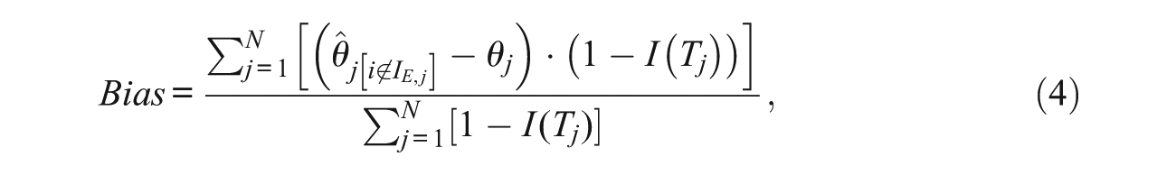
Because this methodology estimates θ using only a subset of items, it is first necessary to demonstrate that this approach does not introduce bias into the θ estimation, and that θ can be estimated with sufficient precision. Using all examinees for whom tampering was not simulated, we estimated the bias and root mean square error (RMSE) on θ as follows:

Bias = \frac{\sum_{j = 1}^{N} [({\hat{θ}}_{j [i \notin I_{E, j}]} - θ_{j}) \cdot (1 - I (T_{j}))]}{\sum_{j = 1}^{N} [1 - I (T_{j})]},

and

RMSE = \sqrt{\frac{\sum_{j = 1}^{N} [{({\hat{è}}_{j [i \notin I_{E, j}]} - θ_{j})}^{2} \cdot (1 - I (T_{j}))]}{\sum_{j = 1}^{N} [1 - I (T_{j})]}},

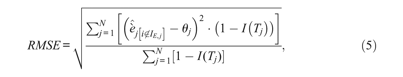
where I(T_j) is an indicator function which equals 1 when the responses for examinee j were tampered, and 0 otherwise. The results are shown in Table 1. Results for the 0 erasures condition serves as a baseline against which to compare the results from the other conditions.

Table 1.

Person Parameter Biases and Root Mean Square Errors.

				Tampered examinees
	Nontampered examinees				Nonerased items only		All items
# Erasures	# Simulees	Bias	RMSE	# Simulees	Bias	RMSE	Bias	RMSE
0	355,611	−0.0137	0.3059	0	—	—	—	—
1	361,511	−0.0137	0.3092	0	—	—	—	—
2	180,882	−0.0149	0.3124	410	0.1259	0.3279	0.2092	0.3647
3	58,875	−0.0137	0.3154	507	0.1465	0.3587	0.2386	0.4002
4	14,283	−0.0149	0.3217	346	0.1596	0.3561	0.2740	0.4225
5	2,838	−0.0099	0.3256	2,246	0.2312	0.4162	0.4385	0.5550
6	616	−0.0352	0.3338	2,089	0.2520	0.4228	0.4644	0.5718
7	589	−0.0046	0.3197	1,107	0.2816	0.4800	0.5082	0.6366
8	929	−0.0045	0.3212	519	0.4121	0.6271	0.6739	0.8279
9	1,454	−0.0211	0.3390	351	0.6229	0.8516	0.9557	1.1136
10	1,618	−0.0234	0.3351	2,407	0.5330	0.6832	0.9535	1.0330
11	1,309	−0.0266	0.3454	1,918	0.5503	0.7094	0.9810	1.0659
12	692	−0.0093	0.3543	901	0.5973	0.7751	1.0485	1.1487
13	305	−0.0210	0.3274	395	0.8045	1.0106	1.2780	1.4069
14	206	−0.0106	0.3315	286	1.0558	1.2606	1.5778	1.7093
≥15	282	−0.0238	0.3652	4,518	0.7921	0.9402	1.4611	1.5299

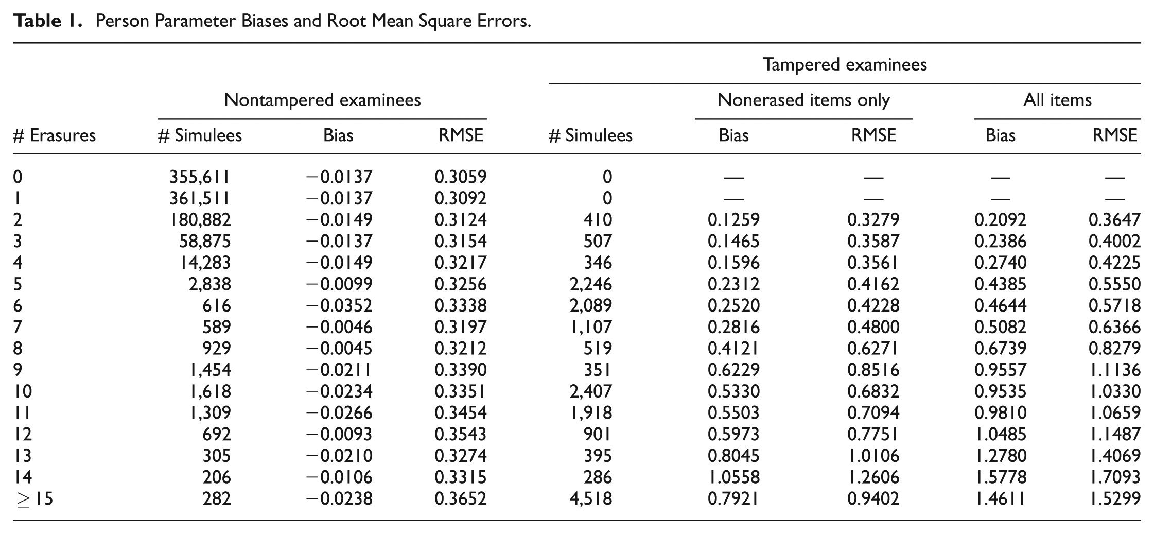
As expected, biases are negligible, even for simulees with as many as 15 benign erasures. Because θ is estimated from fewer and fewer items as the number of erasures continues, it was expected that the standard error of estimation would increase slightly. The expected pattern is observed in the RMSEs, which increase as the number of erasures increases. However, even when θ is estimated from 35 or fewer items, the estimate is only slightly more variable than when all 50 items were used.

For comparison’s sake, the biases and RMSEs are also shown in Table 1 for tampered examinees. With tampered examinees, because the items which are excluded from the estimation are overwhelmingly items that were answered incorrectly by the examinee, systematically removing them and estimating θ across the remaining items (which are more likely to be answered correctly) should result in estimates that are positively biased (i.e., larger than they should be). However, it was anticipated that the amount of positive bias resulting from including the tampered responses would be even larger, thereby providing the justification to estimate θ using only nonerased items.

Table 1 shows the biases and RMSEs for tampered examinees separately based on only the nonerased items and all items as a function of the number of erasures (not all of which were as a result of tampering). The bias and RMSE based on all items were found by replacing ${\hat{θ}}_{j [i \notin I_{E, j}]}$ in (4) and (5) with ${\hat{θ}}_{j}$ .

As expected, θ estimates for tampered examinees include noticeable amounts of positive bias, and both bias and RMSE increase sharply as the number of erasures increase. However, it is also clear that excluding all erased items from the estimation process substantially reduces the bias and RMSEs. Biases are reduced by 33% to 47% and RMSEs are reduced between 10% and 39% when only unerased items are used for estimating θ.

To examine the effect of this purification technique for examinees of different ability levels, biases and RMSEs are broken down by quintile group in Table 2. Because of some small sample sizes in particular Number of Erasures × Quintile subgroups, for purposes of Table 2, the number of erasures are collapsed into six groups.

Table 2.

Person Parameter Biases and Root Mean Square Errors by Quintile Group.

					Tampered examinees
		Nontampered examinees				Nonerased items only		All items
# Erasures	Quintile	# Simulees	Bias	RMSE	# Simulees	Bias	RMSE	Bias	RMSE
0-1	1	143,103	0.0994	0.2786	0	—	—	—	—
	2	143,175	0.0442	0.2697	0	—	—	—	—
	3	143,285	0.0117	0.2776	0	—	—	—	—
	4	144,057	−0.0366	0.2980	0	—	—	—	—
	5	143,502	−0.1868	0.3959	0	—	—	—	—
2-4	1	50,760	0.1041	0.2847	0	—	—	—	—
	2	50,639	0.0450	0.2740	260	0.1500	0.3311	0.2731	0.4012
	3	50,581	0.0121	0.2825	931	0.1231	0.3214	0.2074	0.3563
	4	50,788	−0.0378	0.3017	0	—	—	—	—
	5	51,272	−0.1946	0.4050	72	0.3822	0.6290	0.5207	0.7209
5-7	1	799	0.1223	0.3058	929	0.2280	0.3525	0.4973	0.5590
	2	835	0.0360	0.2864	1,461	0.2050	0.3617	0.4225	0.5118
	3	790	0.0155	0.2846	993	0.2023	0.3798	0.3970	0.5085
	4	795	−0.0334	0.3068	928	0.2680	0.4547	0.4609	0.5835
	5	824	−0.2012	0.4263	1,131	0.3506	0.5764	0.5450	0.7148
8-10	1	798	0.1164	0.2900	671	0.3098	0.4337	0.7943	0.8485
	2	812	0.0448	0.2939	730	0.3546	0.4911	0.7433	0.8189
	3	784	0.0220	0.2987	526	0.4978	0.6271	0.8720	0.9555
	4	783	−0.0205	0.3155	555	0.6232	0.8242	0.9802	1.1231
	5	824	−0.2468	0.4400	795	0.8063	0.9355	1.1346	1.2320
11-13	1	456	0.1145	0.3091	896	0.3643	0.4742	0.8992	0.9403
	2	449	0.0593	0.3003	528	0.4137	0.5331	0.8454	0.9030
	3	455	0.0167	0.3243	527	0.5068	0.6513	0.9052	0.9884
	4	480	−0.0499	0.3174	598	0.8062	1.0181	1.0212	1.3522
	5	466	−0.2364	0.4524	665	0.9284	1.0371	1.3287	1.4084
≥14	1	79	0.1127	0.3256	1,504	0.4887	0.5954	1.3161	1.3629
	2	90	0.0923	0.3048	1,021	0.6740	0.7841	1.3041	1.3576
	3	102	0.0574	0.2811	1,023	0.9390	1.0829	1.5241	1.6101
	4	99	−0.0538	0.3593	919	1.2292	1.3346	1.7829	1.8518
	5	118	−0.2257	0.4384	337	1.0894	1.1567	1.6146	1.6623

For nontampered examinees, Table 2 shows that that θ estimates include small degrees of positive bias for the lowest scoring examinees and positive bias for the highest scoring examinees. This bias at the extremes of the θ distribution is likely attributable to shrinkage toward a mean θ of zero, as is customary with default MAP estimates in MULTILOG (Thissen & Orlando, 2001). There does not appear to be a noteworthy relationship between the number of benign erasures and the shrinkage effect.

For tampered examinees, however, Table 2 shows that bias and RMSE are reduced for all quintile groups when θ is estimated using only nonerased items; however, the largest reductions are for the examinees in the lower quintile groups. Collapsed across all examinees, the average percentage reduction in bias is 60%, 50%, 43%, 33%, and 32% for Quintiles 1, 2, 3, 4, and 5, respectively. Similarly, RMSEs were reduced, on average, by 49%, 35%, 26%, 25%, and 23% for Quintiles 1 through 5, respectively.

Taken together, these results suggest that excluding erased items from the estimation of θ serves to partially neutralize the effect of tampering and improves the quality of estimation, while its effects on nontampered examinees are negligible, even if the number of erasures is high. The effects of this purification approach are most pronounced for low-ability examinees, which are precisely the examinees for whom tampering is most likely. Consequently, this approach was used throughout this study to estimate θ.

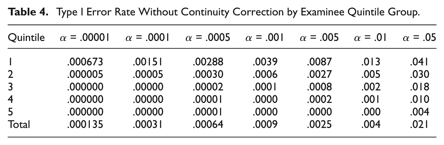
Type I error results are provided when continuity correction is not used for each of the five quintile groups within each benign erasure condition in Table 3, and collapsed across benign erasure conditions in Table 4. From the bottom row of Table 4, one can see that collapsed across erasure type and quintile groups, the overall Type I error rate is well controlled, except for the very smallest α levels. However, the bodies of Tables 3 and 4 both show significant degrees of α inflation in several conditions. In particular, Type I error rates exceed nominal levels as α levels decrease, for lower quintile groups. This is particularly true in misalignment and string-end conditions. Given that, in practice, test tampering is most likely to occur with lower ability examinees and that data forensic techniques are typically applied with conservative α levels, the results of Tables 3 and 4 are troubling.

Table 3.

Type I Error Rate Without Continuity Correction by Benign Erasure Type and Examinee Quintile Group.

Benign erasure	Quintile	α = .00001	α = .0001	α = .0005	α = .001	α = .005	α = .01	α = .05
Misalignment	1	.000000	.00128	.00640	.0077	.0141	.024	.056
	2	.000000	.00000	.00128	.0013	.0064	.010	.052
	3	.000000	.00000	.00000	.0000	.0013	.006	.046
	4	.000000	.00000	.00000	.0000	.0064	.014	.081
	5	.000000	.00000	.00000	.0000	.0013	.010	.076
Random
	1	.000674	.00151	.00287	.0039	.0087	.013	.041
	2	.000000	.00004	.00027	.0005	.0026	.005	.030
	3	.000000	.00000	.00002	.0001	.0008	.002	.018
	4	.000000	.00000	.00001	.0000	.0001	.000	.009
String-end	5	.000000	.00000	.00000	.0000	.0000	.000	.003
	1	.001287	.00129	.00129	.0026	.0129	.017	.055
	2	.001280	.00256	.00512	.0051	.0128	.019	.065
	3	.000000	.00000	.00000	.0026	.0090	.022	.077
	4	.000000	.00000	.00000	.0000	.0088	.019	.066
	5	.000000	.00000	.00126	.0013	.0013	.008	.085

Table 4.

Type I Error Rate Without Continuity Correction by Examinee Quintile Group.

Quintile	α = .00001	α = .0001	α = .0005	α = .001	α = .005	α = .01	α = .05
1	.000673	.00151	.00288	.0039	.0087	.013	.041
2	.000005	.00005	.00030	.0006	.0027	.005	.030
3	.000000	.00000	.00002	.0001	.0008	.002	.018
4	.000000	.00000	.00001	.0000	.0002	.001	.010
5	.000000	.00000	.00001	.0000	.0000	.000	.004
Total	.000135	.00031	.00064	.0009	.0025	.004	.021

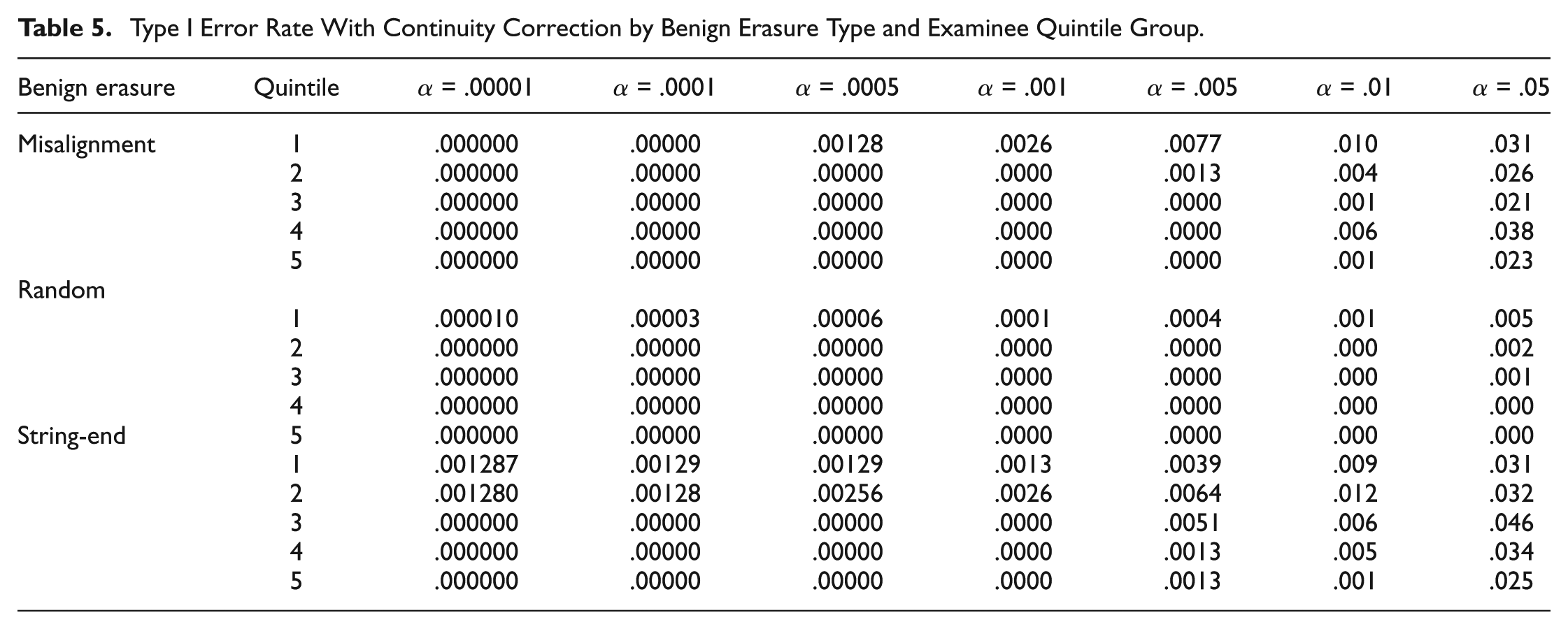
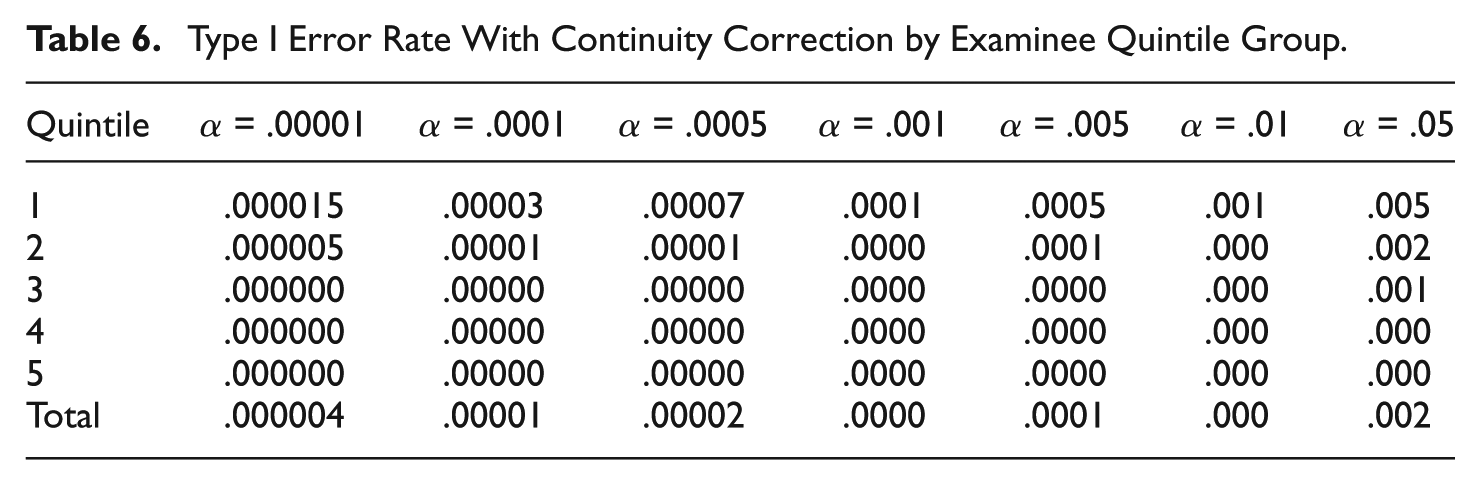
The same data are provided in Tables 5 and 6 when continuity correction is applied. Inspection of Table 5 shows that the false positive rate is well-controlled, if not quite conservative, in nearly all conditions. The few conditions in which there is apparent inflation—for quintiles 1 and 2 at the smallest α levels in the string-end condition—are likely a product of the fact that insufficient string-end erasures were simulated to allow accurate estimation of such small α levels. In fact, the inflated error rates are attributable to a very small number of detected simulees (just 1 in the case of the α = .00001 and .0001 conditions). Because error rates were lowest for the random erasure conditions, when the Type I error rates are collapsed across the three types of erasures, error rates are quite conservative in all conditions.

Table 5.

Type I Error Rate With Continuity Correction by Benign Erasure Type and Examinee Quintile Group.

Benign erasure	Quintile	α = .00001	α = .0001	α = .0005	α = .001	α = .005	α = .01	α = .05
Misalignment	1	.000000	.00000	.00128	.0026	.0077	.010	.031
	2	.000000	.00000	.00000	.0000	.0013	.004	.026
	3	.000000	.00000	.00000	.0000	.0000	.001	.021
	4	.000000	.00000	.00000	.0000	.0000	.006	.038
	5	.000000	.00000	.00000	.0000	.0000	.001	.023
Random
	1	.000010	.00003	.00006	.0001	.0004	.001	.005
	2	.000000	.00000	.00000	.0000	.0000	.000	.002
	3	.000000	.00000	.00000	.0000	.0000	.000	.001
	4	.000000	.00000	.00000	.0000	.0000	.000	.000
String-end	5	.000000	.00000	.00000	.0000	.0000	.000	.000
	1	.001287	.00129	.00129	.0013	.0039	.009	.031
	2	.001280	.00128	.00256	.0026	.0064	.012	.032
	3	.000000	.00000	.00000	.0000	.0051	.006	.046
	4	.000000	.00000	.00000	.0000	.0013	.005	.034
	5	.000000	.00000	.00000	.0000	.0013	.001	.025

Table 6.

Type I Error Rate With Continuity Correction by Examinee Quintile Group.

Quintile	α = .00001	α = .0001	α = .0005	α = .001	α = .005	α = .01	α = .05
1	.000015	.00003	.00007	.0001	.0005	.001	.005
2	.000005	.00001	.00001	.0000	.0001	.000	.002
3	.000000	.00000	.00000	.0000	.0000	.000	.001
4	.000000	.00000	.00000	.0000	.0000	.000	.000
5	.000000	.00000	.00000	.0000	.0000	.000	.000
Total	.000004	.00001	.00002	.0000	.0001	.000	.002

The power of EDI without continuity correction is shown in Tables 7, and with continuity correction in Table 8. Note that power data are only provided for those conditions for which the Type I error rate was not liberal. Power without the continuity correction is, not surprisingly, noticeably higher. However, even when the correction is applied, the power of EDI is quite high to detect small amounts of tampering among first quintile simulees. By the time 10 WTR erasures are observed, detection rates are very strong, even at small α levels. When the correction is not applied, the power is outstanding, detecting nearly every first quintile student when α = .01 or higher, even when only 5 items are erased. The power among first quintile students without the correction cannot be evaluated at most α levels because the Type I error rates are inflated. At higher α levels, the power without continuity correction remains excellent into the second, and even third quintile groups; however, beginning around α = .001, power drops off considerably for the higher quintile groups. From Table 8, one can see that power drops off considerably for second quintile students at smaller α levels when continuity correction is applied, but detection rates are still very strong at higher α levels and when 10 or more erasures are observed. Power continues to decrease into and beyond the third quintile. Detection rates are still reasonable for third quintile students at the highest α levels provided 10 to 15 items are changed. However, detection rates are unimpressive all around for the fifth quintile simulees. This is likely attributable to the fact that examinees in this category were high achieving, and in many cases, their raw scores were sufficiently close to 50 (the maximum) that it was not possible to change as many as 10 or 15 items from incorrect to correct. Consequently, those examinees did not experience the full effect of the condition in which they were placed. Fortunately, the lower power in the upper quintiles presents little practical difficulty, because administrators are much less likely to tamper with the answer sheets of top students.

Table 7.

Power Without Continuity Correction.

Amount of tampering	Quintile	α = .00001	α = .0001	α = .0005	α = .001	α = .005	α = .01	α = .05
5 Erasures	1	—	—	—	—	—	.914	.987
	2	.018	.058	.179	.262	.554	.683	.923
	3	.000	.008	.031	.065	.265	.443	.831
	4	.000	.000	.004	.010	.076	.190	.668
	5	.000	.000	.000	.000	.007	.028	.367
10 Erasures
	1	—	—	—	—	—	.995	.999
	2	.171	.418	.666	.757	.921	.965	.996
	3	.010	.085	.242	.359	.702	.836	.976
	4	.004	.009	.053	.086	.342	.533	.922
15 Erasures	5	.000	.000	.000	.002	.038	.095	.590
	1	—	—	—	—	—	1.000	1.000
	2	.331	.604	.795	.871	.976	.991	1.000
	3	.043	.166	.338	.446	.748	.847	.983
	4	.003	.011	.044	.077	.259	.425	.911
	5	.000	.000	.001	.002	.021	.042	.614
Score-based	1	—	—	—	—	—	.995	.999
	2	.041	.129	.244	.321	.503	.607	.826
	3	.000	.000	.001	.007	.052	.095	.424
	4	NA	NA	NA	NA	NA	NA	NA
	5	NA	NA	NA	NA	NA	NA	NA

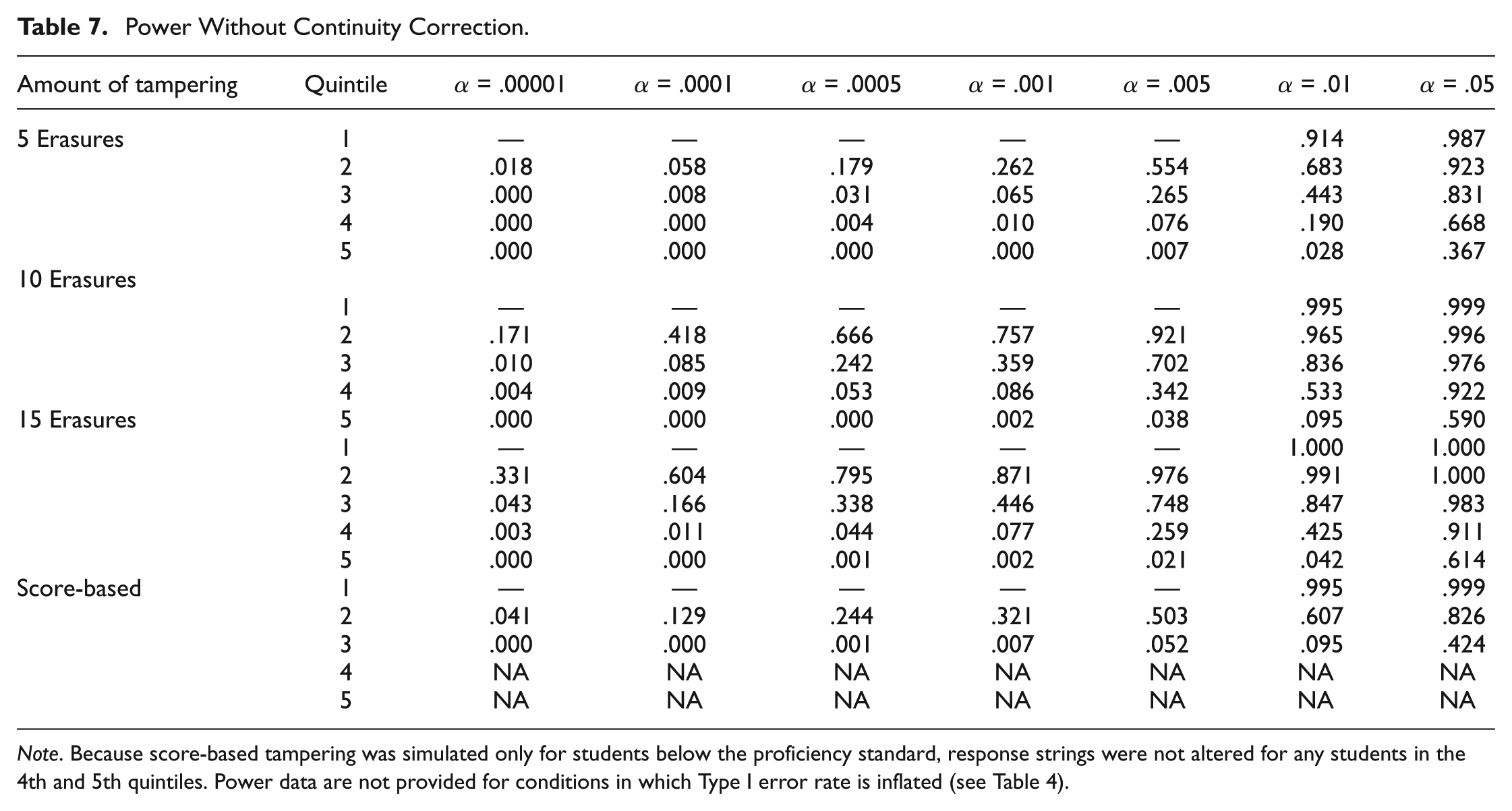
Note. Because score-based tampering was simulated only for students below the proficiency standard, response strings were not altered for any students in the 4th and 5th quintiles. Power data are not provided for conditions in which Type I error rate is inflated (see Table 4).

Table 8.

Power With Continuity Correction.

Amount of tampering	Quintile	α = .00001	α = .0001	α = .0005	α = .001	α = .005	α = .01	α = .05
5 Erasures	1	.140	.258	.385	.458	.676	.765	.961
	2	.005	.018	.046	.075	.287	.420	.794
	3	.000	.001	.007	.014	.081	.162	.605
	4	.000	.000	.000	.000	.011	.035	.304
	5	.000	.000	.000	.000	.000	.000	.086
10 Erasures
	1	.587	.779	.888	.927	.980	.991	.999
	2	.077	.250	.473	.584	.834	.904	.990
	3	.003	.032	.122	.188	.460	.641	.934
	4	.002	.005	.014	.033	.150	.283	.759
15 Erasures	5	.000	.000	.000	.000	.009	.030	.262
	1	.832	.939	.977	.986	.998	1.000	1.000
	2	.219	.466	.676	.766	.931	.972	.999
	3	.018	.088	.216	.299	.574	.727	.944
	4	.001	.007	.017	.033	.148	.238	.662
	5	.000	.000	.000	.001	.008	.020	.192
Score-based	1	.681	.829	.907	.932	.977	.990	.998
	2	.019	.055	.129	.175	.348	.419	.662
	3	.000	.000	.000	.000	.001	.013	.096
	4	NA	NA	NA	NA	NA	NA	NA
	5	NA	NA	NA	NA	NA	NA	NA

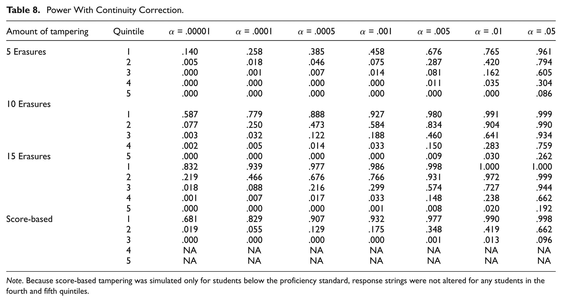
Note. Because score-based tampering was simulated only for students below the proficiency standard, response strings were not altered for any students in the fourth and fifth quintiles.

The score-based condition provides an indication of detection rates in the most egregious of tampering situations in which administrators alter students’ answers just enough to ensure that they will score at the proficient level. The median numbers of erasures were 13 and 5 for students in the first and second quintiles, respectively. Because of where the proficiency cut-score was set, even the weakest of the third quintile simulees were very close to the cut-score. As a result, all third quintile examinees selected were only one raw score point below the cutoff. Because this condition erased enough items to raise scores to one point above the proficiency cutoff, all third quintile students in this condition had only two items erased.

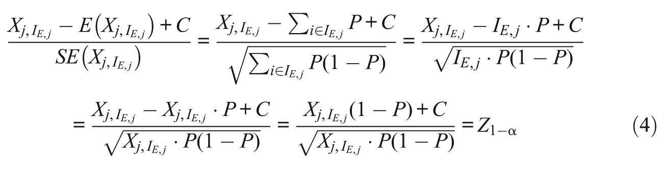
The strong power of EDI can be explained analytically. Computation of EDI involves three components: the number correct score on erased items, the expected number correct score, and the standard error. However, within the test tampering framework, erasures will overwhelmingly be WTR erasures. Given that benign erasures are relatively rare, the number correct score on the erased items, $X_{j, I_{E, j}},$ is almost always the same as the number of erased items, $I_{E, j}$ . Inserting (1) and (2) into (3), under the assumptions that all items are equally difficult and that no benign erasures exist (i.e., $I_{E, j} = X_{j, I_{E, j}})$ , it is possible to find the average probability of correct response, P, below which would produce statistically significant EDI values. That is, under these simplifying conditions,

\frac{X_{j, I_{E, j}} - E (X_{j, I_{E, j}}) + C}{SE (X_{j, I_{E, j}})} = \frac{X_{j, I_{E, j}} - \sum_{i \in I_{E, j}} P + C}{\sqrt{\sum_{i \in I_{E, j}} P (1 - P)}} = \frac{X_{j, I_{E, j}} - I_{E, j} \cdot P + C}{\sqrt{I_{E, j} \cdot P (1 - P)}} = \frac{X_{j, I_{E, j}} - X_{j, I_{E, j}} \cdot P + C}{\sqrt{X_{j, I_{E, j}} \cdot P (1 - P)}} = \frac{X_{j, I_{E, j}} (1 - P) + C}{\sqrt{X_{j, I_{E, j}} \cdot P (1 - P)}} = Z_{1 - α}

where Z_1−α is the value under the normal distribution corresponding to the 100 × (1 −α) percentile.

For fixed values of $X_{j, I_{E, j}}$ and α, this equation can easily be solved for p. Table 9 shows the values of p that solve (4) for 5, 10, and 15 erasures, and each of the seven α levels examined in this study, both with and without continuity correction. As an example, when α = .05 and continuity correction is not used, if 5 items are erased, simulees will be detected for whom the average probability of correct response across those erased items is 0.649 or lower. For examinees in the lower quintile groups, unless the erased items happen to be very easy, it is unlikely that they will have an average probability of correct response as high as 0.649, thus leading to a significant EDI index. However, for examinees in the upper quintile groups, unless the items are very hard, it is quite likely that their probability of answering the erased items correctly will be greater than 0.649, leading to a lack of significance. As expected, the critical p value decreases as α decreases, requiring the erased items to be, on average, more difficult for the examinees to lead to detection. Similarly, as the number of erased items increases, the critical P value increases, making detection increasingly likely. Also, Table 9 can be used to better understand the differences in expected power as a function of using continuity correction. For most α levels, adding continuity correction means that the average item difficulty needed for significance will be .05 to .07 lower than when no correction is used, thereby making it more difficult to detect.

Table 9.

Average Probability of Correct Response Below Which Yields Statistical Significance.

# Erasures	α = .00001	α = .0001	α = .0005	α = .001	α = .005	α = .01	α = .05
A. Without correction for continuity
5	0.215	0.266	0.316	0.344	0.430	0.480	0.649
10	0.354	0.420	0.480	0.512	0.601	0.649	0.787
15	0.451	0.520	0.581	0.611	0.693	0.735	0.847
B. With correction for continuity
5	0.175	0.216	0.257	0.280	0.350	0.392	0.533
10	0.320	0.379	0.434	0.463	0.544	0.588	0.715
15	0.422	0.487	0.543	0.572	0.649	0.688	0.795

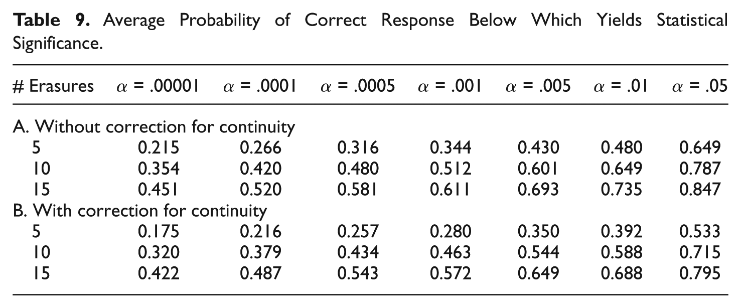
It is worth noting that the assumption of equally difficult items is undoubtedly false. However, of the three components involved in the computation of EDI, varying item difficulties will affect only the standard error. However, for a fixed expected value, the special case in which all items are equally difficult produces the largest standard error, hence the smallest EDI. Therefore, to the extent that the equal difficulty assumption is false, EDI values will be larger, making it even easier to flag students. Therefore, if the average probabilities are equal to the values in Table 9, even if the assumption of equal difficulty is violated, the student is certain to be flagged.

The presence of benign erasures, however, would likely have an impact on the data in Table 9. To the extent that fraudulent erasures are accompanied by some benign erasures that lead to incorrect answers among the erased set, both the expected values and the standard error are likely to increase, making the EDI index less extreme and necessitating items that are harder than reported in Table 9 in order to detect.

Discussion

The EDI index developed here looks to be a very promising tool for detection of test tampering. The results of this study show that the normal approximation approach produced good overall control of the nominal Type I error rate; however, in order to maintain control for the lowest scoring examinees—the ones most likely to be erasure victims—it is necessary to apply a correction for continuity. Even when that correction is applied, the EDI demonstrates strong power to detect test tampering among the lowest achieving students, and respectable power for the second quintile students in the 10- and 15-erasure conditions. In practice, the low power to detect test tampering among high-achieving students is of little consequence, as test tampering is much less likely to occur for high-achieving students. Furthermore, the validity of the test score interpretation is compromised much less with high-ability students than with low-ability students. While ethical reasons suggest that we are still interested in detecting all cheating, even if by high-achieving students, we must recall that in the case of test tampering, it is not the student who is ethically challenged, but the individual who changed the answers. Fortunately, administrators who change answers for high-achieving students likely do similarly for low-achieving students, so other opportunities exist for them to be detected.

One limitation of this study is that, for purposes of demonstrating the efficacy of the model, all analyses were based on item parameters which, by virtue of being parameters, were (a) free from random error and (b) uncontaminated by the effects of tampering. In practice, item parameters will be estimated from the data and to the extent that test tampering existed in the data set, the parameter estimates would be somewhat contaminated. Although this study did not investigate the impact of these sources of error, the effects of both are known. Because the EDI follows the same functional form as the answer copying index, ω (Wollack, 1997), research on the impact of estimating item parameters within the context of data contaminated with varying magnitudes of answer copying generalizes to the present study. Wollack and Cohen (1998) found that replacing item parameters with item parameter estimates partially contaminated by the effects of cheating did not affect the Type I error rates of the ω index. They also found that power was reduced a small amount when sample size was small (e.g., N = 100), but was virtually unchanged for sample sizes of 500. Within the present context of a statewide erasure analysis, sample sizes will always be much larger than 500, so Type I error rate and power are expected to be unaffected. Similarly, the extent of test tampering across an entire state figures to be very small (e.g., a modest proportion of answers for a small proportion of students for a small proportion of teachers within a small proportion of schools). Furthermore, there is no reason to believe that different educators would tamper with the same items (at least across schools). Therefore, the amount of tampering on each question is expected to be minimal. It is not anticipated that realistic amounts of tampering will have any effect on the values of the item parameter estimates.

It is worth noting that the method proposed here is for detection of individuals. However, in practice, testing programs are likely more interested in detecting tampering at the group level than at the individual level. Fortunately, the EDI is easily adapted to a group-level context, and the authors are beginning to study models to aggregate EDI to detect tampering at the class, school, or district level.

Finally, it is likely that EDI would have somewhat better control of the false–positive rate and power if the exact generalized binomial model were used, rather than the normal approximation test used here. van der Linden and Sotaridona (2006) have demonstrated this result with the ω answer copying statistic. However, the normal approximation is computationally much more straightforward, thereby providing an index that is more accessible to school districts that may not have the measurement or programming expertise necessary to derive the compound binomial probabilities. The results of this study suggest that the user-friendly form of the EDI used here has sufficient power and Type I error control that whatever increases in power may be achieved by the exact test are likely offset by the increased complexity which would serve to discourage its use.

As with any data forensic tool, it is important to note that the EDI is a statistical procedure, and false positives will occasionally occur. An accusation of test tampering is very serious, and figures to have negative financial, social, and legal implications on the individuals involved. Therefore, while data forensics should be run routinely to flag potential instances of tampering or other forms of cheating, such statistical procedures should never represent the entirety of the investigation. Whenever suspicious test results are found, it is incumbent on the district/state to conduct a full investigation aimed both at uncovering additional information to support an allegation of misconduct and providing alternative explanations for the anomalous statistical findings. Only after a complete investigation has occurred and alternative explanations have been discounted can one conclude that the findings are indicative of cheating.

Footnotes

Declaration of Conflicting Interests

The author(s) declared no potential conflicts of interest with respect to the research, authorship, and/or publication of this article.

Funding

The author(s) received no financial support for the research, authorship, and/or publication of this article.

References

Allen

(2012). Relationships of examinee pair characteristics and item response similarity (ACT Research Report Series, 2012(8)). Retrieved from http://www.act.org/research/researchers/reports/pdf/ACT_RR2012-8.pdf

Asimov

Wallack

(2007, May 13). The teachers who cheat/Some help students during standards test—or fix answers later—and California’s safeguards may leave more breaches unreported. San Francisco Chronicle. Retrieved from http://www.sfgate.com/education/article/THE-TEACHERS-WHO-CHEAT-Some-help-students-2560689.php

Bishop

N. S.

Liassou

Bulut

Seo

D. G.

Bishop

(2011, April). Modeling erasure behavior. Paper presented at the annual meeting of the National Council on Measurement in Education, New Orleans, LA.

Bock

R. D.

(1972). Estimating item parameters and latent ability when responses are scored in two or more nominal categories. Psychometrika, 46, 443-459.

Hanson

B. A.

Harris

D. J.

Brennan

R. L.

(1987). A comparison of several statistical methods of examining allegations of copying (ACT Research Report Series, 87-15). Iowa City, IA: ACT.

Hull

(2008). The proficiency debate: At a glance. Retrieved from http://www.centerforpubliceducation.org/Main-Menu/Evaluating-performance/The-proficiency-debate-At-a-glance/

Kingston

(2013). Educator cheating and the statistical detection of group-based test security threats. In Wollack

J. A.

Fremer

J. J.

(Eds.), Handbook of test security (pp. 299-311). New York, NY: Routledge.

Maynes

(2013). Educator cheating and the statistical detection of group-based test security threats. In Wollack

J. A.

Fremer

J. J.

(Eds.), Handbook of test security (pp. 173-199). New York, NY: Routledge.

McGraw

Woo

(1988, September 8). More schools checked for cheating. Los Angeles Times. Retrieved from http://articles.latimes.com/1988-09-08/local/me-2308_1_elementary-schools

10.

Mroch

A. A.

Huang

C.-Y.

Harris

D. J.

(2012, May). Patterns of erasure behavior for a large-scale assessment. Paper presented for the Conference on the Statistical Detection of Potential Test Fraud, Lawrence, KS.

11.

Primoli

Liassou

Bishop

N. S.

Nhouyvanisvong

(2011, April). Erasure descriptive statistics and covariates. Paper presented at the annual meeting of the National Council on Measurement in Education, New Orleans, LA.

12.

Skorupski

Egan

(2012, May). A hierarchical linear modeling approach for detecting cheating and aberrance. Paper presented at the Conference on the Statistical Detection of Potential Test Fraud, Lawrence, KS.

13.

Thissen

(2003). MULTILOG 7.0: Multiple, categorical item analysis and test scoring using item response theory [Computer program]. Chicago, IL: Scientific Software.

14.

Thissen

Orlando

(2001). Item response theory for items scored in two categories. In Thissen

Wainer

(Eds.), Test scoring (pp. 73-140). Mahwah, NJ: Erlbaum.

15.

van der Linden

W. J.

Jeon

. (2012). Modeling answer changes on test items. Journal of Educational and Behavioral Statistics, 37, 180-199.

16.

van der Linden

W. J.

Sotaridona

(2006). Detecting answer copying when the regular response process follows a known response model. Journal of Educational and Behavioral Statistics, 31, 283-304.

17.

Wollack

J. A.

(1997). A nominal response model approach to detect answer copying. Applied Psychological Measurement, 21, 307-320.

18.

Wollack

J. A.

Cohen

A. S.

(1998). Detection of answer copying with unknown item and trait parameters. Applied Psychological Measurement, 22, 144-152.

19.

Wollack

J. A.

Maynes

(2011, February). Data forensics: What works, what doesn’t. Presentation at the annual meeting of the Association of Test Publishers, Phoenix, AZ.