Hypothesis Testing Using Factor Score Regression

Abstract

In this article, an overview is given of four methods to perform factor score regression (FSR), namely regression FSR, Bartlett FSR, the bias avoiding method of Skrondal and Laake, and the bias correcting method of Croon. The bias correcting method is extended to include a reliable standard error. The four methods are compared with each other and with structural equation modeling (SEM) by using analytic calculations and two Monte Carlo simulation studies to examine their finite sample characteristics. Several performance criteria are used, such as the bias using the unstandardized and standardized parameterization, efficiency, mean square error, standard error bias, type I error rate, and power. The results show that the bias correcting method, with the newly developed standard error, is the only suitable alternative for SEM. While it has a higher standard error bias than SEM, it has a comparable bias, efficiency, mean square error, power, and type I error rate.

Keywords

factor score regression bias standard error standardized parameterization unstandardized parameterization

Introduction

In the social and behavioral sciences, the aim of applied researchers is often to examine the relationships between latent variables. Latent variables are variables that are not directly observable, such as intelligence, skill, or motivation. To measure these latent variables, observable indicators are used (Bollen & Hoyle, 2012). Structural equation modeling (SEM) can be used to simultaneously and consistently estimate both the measurement models and the structural relations between these latent variables (Bentler & Chou, 1987; Jöreskog, 1973). Despite the increasing popularity of SEM, many applied researchers prefer to use the factor score regression (FSR) method, which is more intuitive and consists of two steps. In a first step, the scores on the latent variables are predicted using factor analysis (FA). In this article, we will refer to these predicted scores as factor scores. In a second step, the factor scores are used in a linear regression (ordinary least squares; Lu, Thomas, & Zumbo, 2005). Unfortunately, there are an infinite number of ways to compute these factor scores, all of which are consistent with the FA performed (Grice, 2001), meaning they are all equally viable. The two most commonly used predictors are the regression predictor (Thomson, 1934; Thurstone, 1935) and the Bartlett predictor (Bartlett, 1937; Thomson, 1938). The factor scores will be different depending on which predictor is used. This phenomenon is referred to as factor indeterminacy (Maraun, 1996; Mulaik, 1972; Steiger, 1979). The degree of indeterminacy is small if the relationship between the indicators and the latent variable is strong or if the number of indicators is high (Acito & Anderson, 1986). When there is a high degree of factor indeterminacy, it is even possible for an individual to score high according to the factor scores calculated by one method and score low according to the factor scores of another method (Grice, 2001). Lastovicka and Thamodaran (1991) conclude that indeterminacy implies that factor scores cannot be measured and researchers have to accept that FA means it is impossible to obtain an unambiguous prediction or computation of the latent variable scores. In other words, a degree of uncertainty is inherent to factor scores, which is no longer accounted for when using factor scores in linear regression. This uncertainty causes the regression coefficient to be biased, as has been discussed extensively in the literature (e.g., Bollen, 1989; Lastovicka & Thamodaran, 1991; Lewis & Linzer, 2005; Shevlin, Miles, & Bunting, 1997). Despite its obvious drawbacks, FSR remains a popular method among applied researchers (Lu & Thomas, 2008).

For this reason, improved methods to perform FSR have been developed, which result in an unbiased regression coefficient (Croon, 2002; Skrondal & Laake, 2001). Skrondal and Laake (2001) developed a method which avoids bias altogether, while Croon (2002) found a method to correct for the bias. We will refer to these methods as the bias avoiding and bias correcting method, respectively. Both methods indeed result in an unbiased parameter estimate, but are hardly ever used in practice. This is partly due to the highly technical and mathematical level of the articles describing the methods. Lu, Kwan, Thomas, and Cedzynski (2011) tried to remedy this by giving an overview of both methods. The statistical performance of both methods was also compared in a simulation study, with regard to accuracy and power. However, the methods remain unused by applied researchers. This could be due to some practical issues. First of all, it is only described how to obtain an unbiased estimate for the regression coefficient, but for the bias correcting method, there is no standard error available. This means that this method cannot be used yet to test hypotheses. Second, the results of the methods have only been described for the unstandardized parameterization. Neither Skrondal and Laake (2001), Croon (2002), or Lu et al. (2011) describe what happens when the standardized parameterization is used. In conclusion, the methods are not directly usable for the applied researchers.

The goal of this article is to compare various methods for performing FSR, namely FSR using the regression predictor (regression FSR), FSR using the Bartlett predictor (Bartlett FSR), the method of Skrondal and Laake (2001; bias avoiding method), and the method of Croon (2002; bias correcting method). For each method we derive the bias analytically on the population level for both the standardized and unstandardized parameterization. Next, for the bias correcting method, a new standard error is developed, making it possible to use the bias correcting method to test hypotheses. Finally, two simulation studies are set up to compare the performance of the four methods in finite samples, using normal and nonnormal data, respectively. The simulation studies also allow us to evaluate the performance of the newly developed standard error. Since SEM is generally considered as the standard method to examine the regressions between latent variables, SEM is also included in the simulation studies. The aim is to be able to compare the methods on their overall statistical performance and formulate recommendations for the applied users.

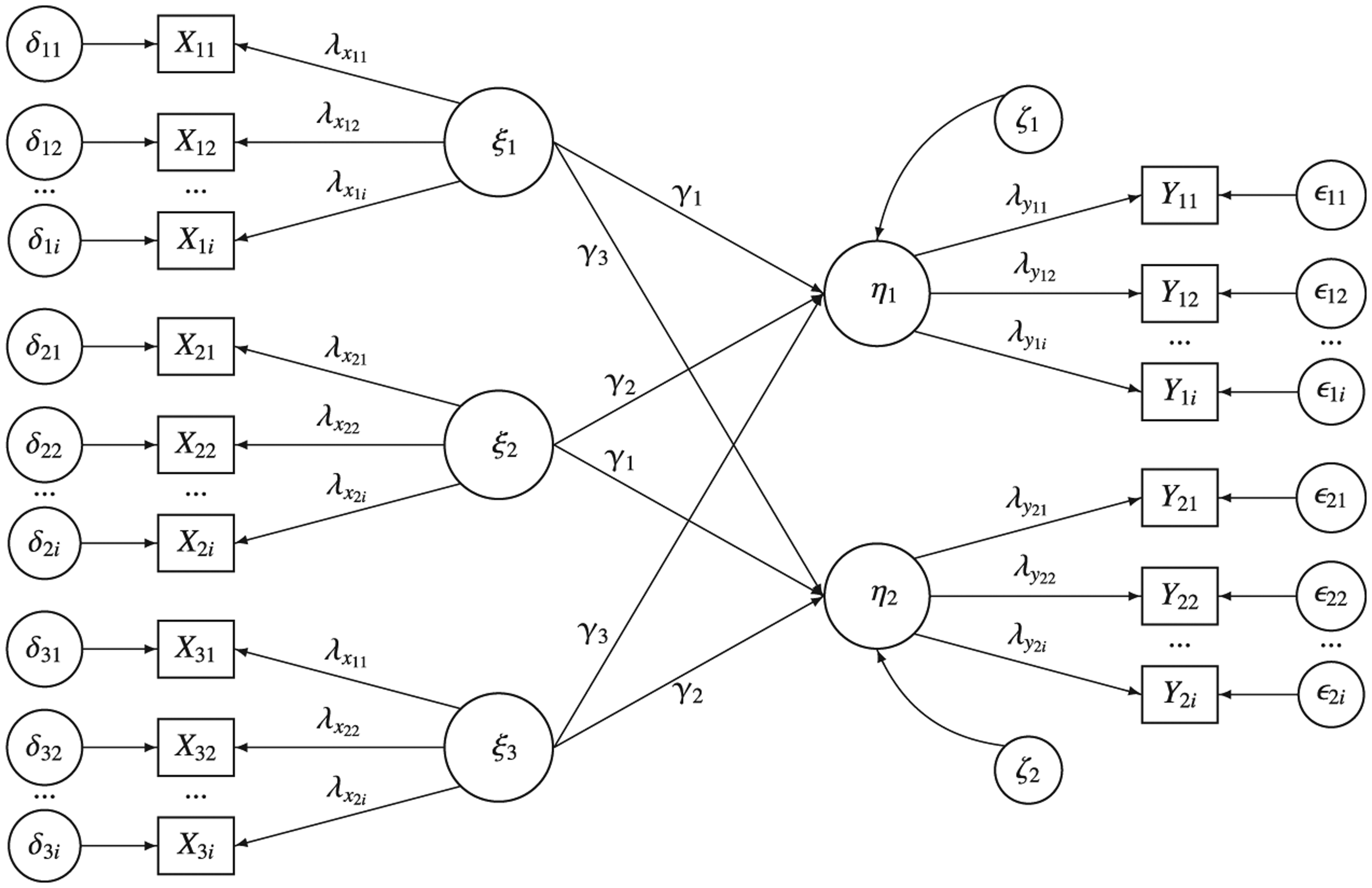
Setting

To be able to compare the four methods, a simple regression model with one dependent and one independent variable is used. The simple regression model is used to reduce the notational complexity and enhance comprehensibility. However, it can easily be extended, to settings with more than one dependent variable and more than one independent variable. In fact, a more complex setting is used in the simulation study. Within this framework of a simple linear regression, we consider four possible scenarios, which are visualized in Figure 1. In the first scenario, both the dependent and independent variable are measured without error. They are considered observed variables. In the second scenario, factor scores are used for the independent variable, while the dependent variable is observed. In the third scenario, factor scores are used for the dependent variable, while the independent variable is observed. In the fourth and final scenario, factor scores are used for both variables. In all scenarios, the structural equation is

η = γ ξ + ζ,

where $η$ is the dependent variable, $ξ$ is the independent variable, $γ$ is the regression coefficient, and $ζ$ is the residual error term. When $η$ and $ξ$ are latent, the following measurement models are used:

x = Λ_{x} ξ + δ

y = Λ_{y} η + ε,

where $x = (X_{1}, . . ., X_{i}, . . ., X_{p})^{T}$ and $y = (Y_{1}, . . ., Y_{j}, . . ., Y_{q})^{T}$ are vectors of mean-centered observed indicators measuring $ξ$ and $η$ respectively, $Λ_{x}$ and $Λ_{y}$ are vectors of the factor loadings and $δ$ and $ε$ are the respective vectors of measurement error variables.

Figure 1.

The four scenarios considered.

In the first step of FSR, we use these measurement models to perform an FA for each latent variable separately and to calculate the factor scores for $ξ$ ( $F_{ξ}$ ) and $η$ ( $F_{η}$ ). To be able to perform a FA, the metric scales of the latent variables $ξ$ and $η$ have to be fixed. This can be done in several ways, for example by fixing one factor loading per latent variable to 1 or by fixing the variance of the latent variable to 1. We will refer to the latter as the standardized parameterization, and the former as the unstandardized parameterization. In this article, we will mainly use the unstandardized parameterization.

The factor scores are calculated by multiplying a factor score matrix $A$ with the observed indicators $x$ (or $y$ ):

F_{η} = A_{η} y

F_{ξ} = A_{ξ} x .

The computation of the factor score matrices $A_{η}$ and $A_{ξ}$ depends on the method used for the prediction of the factor score. The different methods and their influence will be discussed in the next section.

In the second step of FSR, a linear regression is performed between the factor scores, resulting in a regression coefficient. In a simple linear regression, the true regression coefficient is defined as the true covariance between the dependent and the independent variables, divided by the variance of the independent variable:

γ = \frac{cov (ξ, η)}{var (ξ)} .

When performing the linear regression with factor scores, the regression coefficient becomes

β = \frac{cov (F_{ξ}, F_{η})}{var (F_{ξ})},

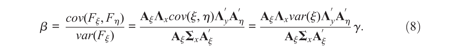
which is not necessarily the same as the true regression coefficient. The relationship between $γ$ and β can best be understood if we work out the covariance and variances of the factor scores. In Appendix A, we derive the exact relationship between β and γ:

β = \frac{cov (F_{ξ}, F_{η})}{var (F_{ξ})} = \frac{A_{ξ} Λ_{x} cov (ξ, η) Λ_{y}^{'} A_{η}^{'}}{A_{ξ} Σ_{x} A_{ξ}^{'}} = \frac{A_{ξ} Λ_{x} var (ξ) Λ_{y}^{'} A_{η}^{'}}{A_{ξ} Σ_{x} A_{ξ}^{'}} γ .

From this, it is clear that in most cases the regression coefficient obtained with FSR will not be the same as the true regression coefficient. It is also possible to calculate the expected regression coefficients when factor scores are only used for one of the variables, dependent or independent. The interested reader can find the calculations in Appendix A.

Methods to Perform Factor Score Regression

To perform FSR, several methods can be used, such as the regression FSR method, the Bartlett FSR method, the bias avoiding method (Skrondal & Laake, 2001) and the bias correcting method (Croon, 2002). In this section, these four methods will be discussed. In Table 1, an overview of this discussion is given.

Table 1.

The Regression Parameter β in Relationship to γ When Using Factor Score Regression.

β =	Both variables observed	Independent variable factor scores, dependent variable observed	Independent variable observed, dependent variable factor scores	Both variables factor scores
The general case	γ	$\frac{A_{ξ} Λ_{x} v a r (ξ)}{A_{ξ} Σ_{x} A_{ξ}^{'}} γ$	$Λ_{y}^{'} A_{η}^{'} γ$	$\frac{A_{ξ} Λ_{x} var (ξ) Λ_{y}^{'} A_{η}^{'}}{A_{ξ} Σ_{x} A_{ξ}^{'}} γ$
Regression FSR	γ	γ	$A_{η}^{R} Λ_{y} γ$	$A_{η}^{R} Λ_{y} γ$
Bartlett FSR	γ	$\frac{var (ξ)}{A_{ξ}^{B} Σ_{x} A_{ξ}^{B'}} γ$	γ	$\frac{var (ξ)}{A_{ξ}^{B} Σ_{x} A_{ξ}^{B'}} γ$
Bias avoiding method	γ	γ	γ	γ
Bias correcting method	γ	γ	γ	γ

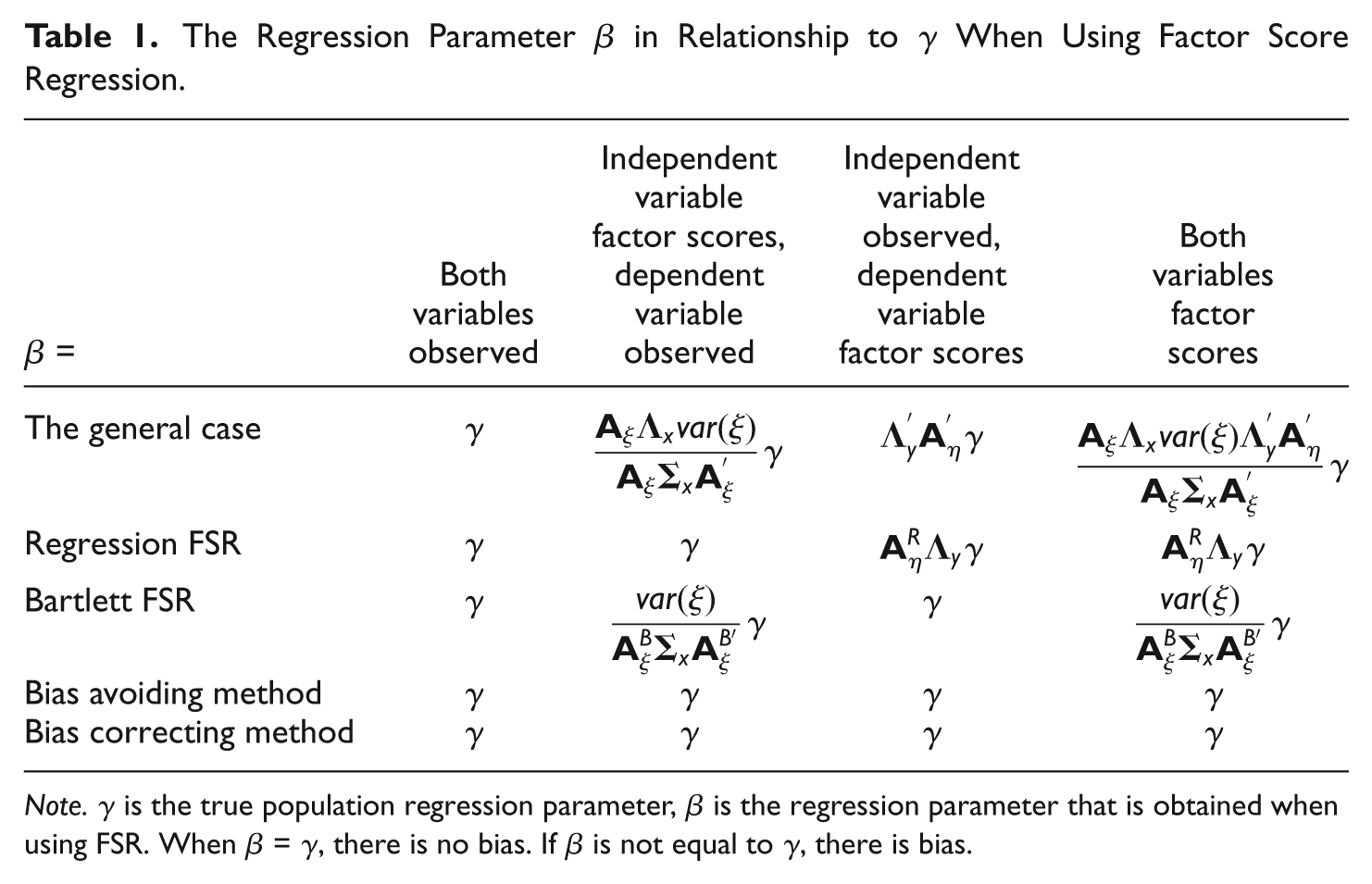
Note. γ is the true population regression parameter, β is the regression parameter that is obtained when using FSR. When β = γ, there is no bias. If β is not equal to γ, there is bias.

Regression Factor Score Regression Method

The regression FSR method uses the regression predictor (Thomson, 1934; Thurstone, 1935) to compute the factor scores and then uses these factor scores in a linear regression. When using the regression predictor, the factor scoring matrices $A_{ξ}^{R}$ and $A_{η}^{R}$ are computed as follows:

A_{ξ}^{R} = Φ Λ_{x}^{'} Σ_{x}^{- 1} = var (ξ) Λ_{x}^{'} Σ_{x}^{- 1},

and

A_{η}^{R} = var (η) Λ_{y}^{'} Σ_{y}^{- 1} .

This means the formula for the variance of $F_{ξ}$ can be simplified. In Appendix B, this is done to show that the regression coefficient in FSR is not biased in all cases. When using the regression FSR method, there is only bias when factor sores are used for the dependent variable. With regard to bias, it is acceptable to use the regression FSR method if only the independent variables are factor scores. When factor sores are used for the dependent variable, one should not use regression FSR, since the regression parameter will be biased in most cases.

These results only apply when the unstandardized parameterization is used (Skrondal & Laake, 2001). The standardized regression coefficient γ_z is different from the unstandardized regression coefficient γ. The standardized regression coefficient can be calculated from the unstandardized regression coefficient and standard deviations:

γ_{z} = \frac{sd (ξ)}{sd (η)} γ .

Since $sd (F_{ξ})$ and $sd (F_{η})$ are biased, the standardized regression coefficient will be biased too if factor scores are used for any of the variables.

Bartlett Factor Score Regression Method

The Bartlett FSR method uses the Bartlett predictor (Bartlett, 1937; Thomson, 1938) to compute the factor scores and then uses these factor scores in a linear regression. The factor scoring matrices $A_{ξ}^{B}$ and $A_{ξ}^{B}$ are calculated as follows:

A_{ξ}^{B} = (Λ_{x}^{'} Θ_{δ}^{- 1} Λ_{x})^{- 1} Λ_{x}^{'} Θ_{δ}^{- 1}

A_{η}^{B} = (Λ_{y}^{'} Θ_{ε}^{- 1} Λ_{y})^{- 1} Λ_{y}^{'} Θ_{ε}^{- 1},

with $Θ_{δ}$ and $Θ_{ε}$ the covariance matrices of respectively, $δ$ and $ε$ .

The Bartlett predictor is less known than the regression predictor, but has the advantage that $A_{ξ}^{B} Λ_{x} = (Λ_{x}^{'} Θ_{δ}^{- 1} Λ_{x})^{- 1} Λ_{x}^{'} Θ_{δ}^{- 1} Λ_{x} = 1$ and $A_{η}^{B} Λ_{y} = 1$ . This implies that the formulas for the covariances can be simplified. The formula for the variance of ξ stays the same. Combined, this gives the regression coefficients as in Appendix C and Table 1. When using Bartlett FSR, there is no longer bias when factor sores are used for the dependent variable. However, now there is bias when factor scores are used for the independent variable. There is also still bias when factor scores are used for both variables.

Again, these results only apply for the unstandardized parameterization. Since the standard deviations are also biased using this method, the standardized regression coefficient will be biased if factor scores are used for any of the variables.

Bias Avoiding Method

The bias avoiding method was developed by Skrondal and Laake (2001). Based on the results discussed in the previous section, they concluded that one should simply use the regression predictor to predict the factor scores of the independent variable, while one should use the Bartlett predictor to predict the factor scores of the dependent variable. It has already been proven that this works for the unstandardized parameterization when factor scores are used for only one of the variables, but Skrondal and Laake (2001) showed that this also works when factor scores are used for both variables. In Appendix D, it is proven that this method results in unbiased estimates for all settings, but it has some drawbacks. First of all, one has to determine in advance if a variable will be dependent or independent. Moreover, a variable can only be dependent or independent. Mediational relationships are not possible. Second, this method only works when the unstandardized parameterization is used. When using the standardized parameterization, the regression coefficient estimate will still be biased.

Bias Correcting Method

The bias correcting method was developed by Croon (2002). In this method, the factor scores are computed using either the regression predictor or the Bartlett predictor. After computing the factor scores, their variances and covariances are calculated. Next, these variances and covariances of the factor scores are used to compute the variances and covariances of the true latent variable scores. Finally, these estimates are used to calculate the regression coefficient. In Appendix E, it is shown how the covariance and variance of the true latent variable scores can be computed. Once these computations have been made, the regression coefficient can be computed as $β = cov (ξ, η) / var (ξ)$ . Since these variances and covariances are unbiased, this results in an unbiased regression coefficient estimate (see Table 1). While this process is more complex than the bias avoiding method, it does have some advantages over it. First of all, it works for both the Bartlett and the regression predictor. Second, since the variances are no longer biased, the standard deviations necessary to calculate the standardized regression coefficient are also unbiased. This means that the method of Croon (2002) also results in an unbiased regression coefficient when the standardized parameterization is used.

Standard Errors

Skrondal and Laake (2001), Croon (2002), and Lu et al. (2011) only describe how to calculate the regression coefficient, just as in the previous section. To be able to use the methods for hypothesis testing, it is necessary to have a complementary significance test, which requires a standard error and a theoretical distribution. For regression FSR, Bartlett FSR and the bias avoiding method, this is no problem. All three methods perform a regular linear regression after calculating the factor scores. This means that the significance test from the linear regression can be used. This test uses the following standard error:

SE = \sqrt{\frac{S^{2}}{\hat{var (F_{ξ})} (n - 1)}},

where S² is defined as:

S^{2} = \hat{var (F_{η})} (1 - r^{2}) \frac{n - 1}{n - (p + 1)},

with $r = γ_{z} = \frac{sd (ξ)}{sd (η)} γ$ , n is the sample size, and p is the number of independent variables. A t-statistic is calculated by dividing the regression coefficient by its standard error. Finally, a p value is calculated by comparing this t-statistic with a t-distribution with n− (p+1) degrees of freedom. Note, that when performing hypothesis tests, we are dealing with finite samples. For this reason, all population parameters are replaced with their corresponding sample estimates.

For the bias correcting method, the standard error is not so easy to calculate. If one would use the above standard error, then this would be the standard error that coincides with the original, uncorrected regression coefficient. In this case, using the corrected regression coefficient to calculate the t value would result in an incorrect t value (and p value). On the other hand, using the uncorrected regression coefficient would just result in a significance test for the uncorrected regression coefficient and is again not adequate.

Another alternative would be to use the above formula for the standard error, but replace all variances and standard deviations with their corrected versions (Croon, 2002). Unfortunately, this approach implicitly assumes that the true latent scores are directly observable, resulting in an underestimation of the standard error. This suggests that the standard error consists of multiple parts, namely error resulting from the regression itself and error resulting from the factor scores. One way to calculate the error resulting from the factor scores, is to first calculate the prediction error in the factor scores. The prediction error in F_ξ and F_η will be denoted as $va r_{ε_{x}}$ and $va r_{ε_{y}}$ , respectively. These prediction errors can be calculated for both the regression and Bartlett predictor. Here, we will only discuss the regression predictor. Skrondal and Rabe-Hesketh (2004, equation 7.7) showed that the prediction errors can be calculated as follows when using the regression predictor:

va r_{ε_{x}} = Φ - Φ^{'} Λ^{'} Σ_{x}^{- 1} ΛΦ

= var (ξ) - var (η) .

The last equation is derived from Equation (B3) in Appendix B. The same derivations can be made for the dependent variable η:

va r_{ε_{y}} = var (η) - var (F_{η}) .

The prediction error in the factor scores is thus the difference between the observed and the corrected variance. Since this is again a variance, the formula from the regular linear regression can be used to calculate the corresponding S². From this, it can be derived that the total S² consists of three parts:

$S_{reg}^{2} = var (η) (1 - r^{2}) \frac{n - 1}{n - (p + 1)}$

$S_{y}^{2} = va r_{ε_{y}} (1 - r^{2}) \frac{n - 1}{n - (p + 1)}$

$S_{x}^{2} = va r_{ε_{x}} r^{2} \frac{n - 1}{n - (p + 1)} .$

Note that for $S_{x}^{2}$ , r² is used instead of 1 −r². This is because the prediction error in the independent variable has more influence on the standard error, as the relation between the variables increases. When the independent variable has no influence on the dependent variable, it also has no influence on the standard error. Now, the total S² can be calculated by summing up the three parts:

S_{total}^{2} = S_{reg}^{2} + S_{y}^{2} + S_{x}^{2} .

Finally, a new adjusted standard error can be calculated as

SE = \sqrt{\frac{S_{total}^{2}}{var (F_{ξ}) (n - 1)}} .

Using this approximate standard error and the corrected regression coefficient, an approximate t statistic can be obtained and compared with the theoretical t-distribution with n− (p+ 1) degrees of freedom. Using this newly developed standard error, the bias correcting method can now be used to perform hypothesis tests about the regression coefficient γ.

Simulation Studies

Two simulation studies are conducted to examine the finite sample performance of these methods and significance tests. In a first study, the methods are studied using item responses that are normally distributed. In the second study, nonnormal item responses are used. The results of these studies can be used as guidelines to determine which method to use, depending on the data and research questions.

First, an outline of how the data were simulated is given, followed by a description of the analyses performed on the simulated data and the results of both studies.

Data Simulation

Study 1

Before the simulation of the data, a ground truth or population model is defined. The structural model consists of a multivariate regression between three latent independent variables, $ξ_{1}$ , $ξ_{2}$ and $ξ_{3}$ , and two latent dependent variables $η_{1}$ and $η_{2}$ , resulting in the structural equation:

η_{1} = γ_{1} ξ_{1} + γ_{2} ξ_{2} + γ_{3} ξ_{3} + ζ_{1},

η_{2} = γ_{3} ξ_{1} + γ_{1} ξ_{2} + γ_{2} ξ_{3} + ζ_{2} .

The model is depicted in Figure 2.

Figure 2.

The population model.

The simulation of the data consists of two steps, which are carried out using R (R Development Core Team, 2008). In the first step, the true latent variable values of $ξ_{1}$ , $ξ_{2}$ , $ξ_{3}$ , $η_{1}$ and $η_{2}$ are generated. The variance of the independent variables $ξ_{1}$ , $ξ_{2}$ and $ξ_{3}$ is set at 100, while the residual variance of the dependent variables $η_{1}$ and $η_{2}$ is set at 400. The covariances between all latent variables are 0. To generate data that comply with these parameters, the true latent scores of $ξ_{1}$ , $ξ_{2}$ and $ξ_{3}$ are first generated, followed by the regression residuals $ζ_{1}$ and $ζ_{2}$ . Finally, using the structural equations $η_{1} = γ_{1} ξ_{1} + γ_{2} ξ_{2} + γ_{3} ξ_{3} + ζ_{1}$ and $η_{2} = γ_{3} ξ_{1} + γ_{1} ξ_{2} + γ_{2} ξ_{3} + ζ_{2}$ , the true latent scores on $η_{1}$ and $η_{2}$ are generated.

In the second step, data are generated for each observed item response x_ij and y_ij, using the true latent scores and the measurement models, with i referring to the latent variables and j to the items. The measurement models of the latent variables are $y_{ij} = λ_{y_{ij}} η_{i} + ε_{ij}$ and $x_{ij} = λ_{x_{ij}} ξ_{i} + δ_{ij}$ . All $λ_{x_{ij}}$ and $λ_{y_{ij}}$ are set at 1. The residual variances $Θ_{ε_{ij}}$ of all y_ij are set at $Θ_{ε_{ij}} = \frac{var (η_{i}) (1 - C D_{y_{i}})}{C D_{y_{i}}}$ and the residual variances $Θ_{δ_{ij}}$ of all x_ij are set at $Θ_{δ_{ij}} = \frac{var (ξ_{i}) (1 - C D_{x_{i}})}{C D_{x_{i}}}$ , with $C D_{y_{i}}$ and $C D_{x_{i}}$ the respective coefficients of determination for the measurement models. All $C D_{x_{i}}$ and $C D_{y_{i}}$ are equal and will thus be referred to as CD. To create item responses that are normally distributed (skewness = 0, kurtosis = 3), ε_ij and δ_ij are generated from a univariate normal distribution.

The coefficient of determination CD, the regression coefficient γ_i, the sample size n, and the number of items I for the two latent variables are varied to create 216 experimental conditions. The sample size is varied to be able to determine the consistency of the methods, while the CD is varied to account for the degree of factor score indeterminacy. A higher CD implies a lower degree of factor score indeterminacy (Acito & Anderson, 1986). The regression coefficient is varied to be able to determine the power and type I error rate. The values used for these parameters can be found in Table 2.

Table 2.

Summary of the Model Parameters Used in Simulation.

Model parameter		Value
Regression coefficients	γ₁	0
	γ₂	1.5
	γ₃	0.41
Coefficient of determination (CD)		0.3, 0.6
		0.7, 0.9
		0.95, 0.99
The sample size (n)		300, 500, 800, 2,000
The number of items (I)		3, 5, 10

Study 2

In the second simulation study, the aim is to compare the methods when the observed item responses are not normally distributed. This means the simulation of the data is done in the same way as in Study 1, except for the generation of the ε_ij and δ_ij. To create nonnormal item responses, the generation of ε_ij and δ_ij is done in two different ways. To create item responses that are symmetrical, but have a large kurtosis, ε_ij and δ_ij are generated from a t-distribution with three degrees of freedom, multiplied by $\sqrt{Θ_{ε_{ij}}}$ or $\sqrt{Θ_{δ_{ij}}}$ , respectively. On average, this results in data with an almost-zero skewness (=0.001) and a kurtosis of about 10.057. To create item responses that are skewed and have a nonnormal kurtosis, ε_ij and δ_ij are generated from χ² -distributions with one degree of freedom, multiplied by $\sqrt{Θ_{ε_{ij}}}$ or $\sqrt{Θ_{δ_{ij}}}$ , respectively. On average, this results in data with a skewness of 0.693 and a kurtosis of 4.785. Note that the way the data are simulated implies that the degree of nonnormality reduces as the CD increases. This is due to the fact that ε_ij and δ_ij have less influence when the factor loadings become stronger.

Analyses

The analysis performed on the data is the same in both studies. Five methods of analyses are performed on the simulated data, namely regression FSR, Bartlett FSR, the bias avoiding method (Skrondal & Laake, 2001), the bias correcting method (Croon, 2002), and SEM.

For the SEM analysis, a correctly specified SEM model is constructed, meaning that it corresponds with the population model used to generate the data. This model is estimated using the simulated data set, with a “maximum likelihood” estimator. From the results, the regression coefficient $\hat{γ}$ , and its standard error SE and p value $\hat{p}$ are obtained, as well as the standardized regression coefficient ${\hat{γ}}_{z}$ . This is done for a 1,000 simulated data sets for every simulation condition. Based on all 1,000 replications, several performance criteria are calculated, namely the mean regression coefficient estimations $\bar{γ}$ and ${\bar{γ}}_{z}$ , the bias using the unstandardized and the bias using standardized parameterization, the empirical standard deviation, the mean square error (MSE), the mean standard error and the standard error bias for the regression coefficient and the power of the statistical test. For the conditions with a regression coefficient of 0, the type I error rate is calculated instead of the power.

For the four FSR methods, an FA is performed for all latent variables. Hereafter, factor scores are calculated, using the Bartlett and the regression predictor. Next, the regression factor scores are used in two linear regressions for the regression FSR and the Bartlett factor scores are used for the Bartlett FSR. For the bias avoiding method, two linear regressions are performed, using the Bartlett factor scores for the dependent variables and the regression factor scores for the independent variables. Finally, for the bias correcting method, the regression coefficient and standard errors are calculated using the formulas described above. 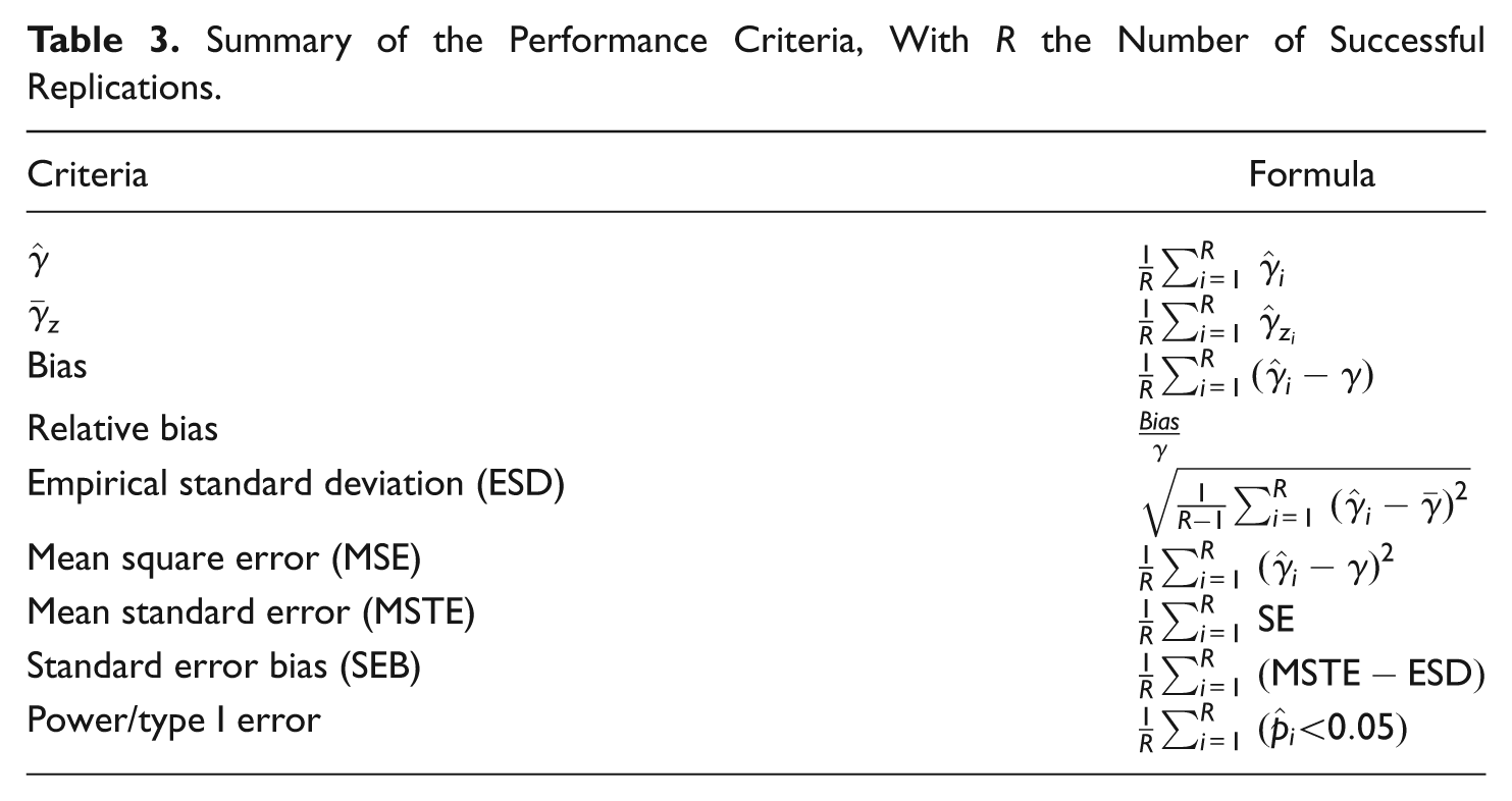Again, the regression coefficients γ and ${\hat{γ}}_{z}$ and the standard error SE and p value $\hat{p}$ for $\hat{γ}$ were retained. This was repeated 1,000 times and the same performance criteria were calculated. The criteria are summarized in Table 3.

Table 3.

Summary of the Performance Criteria, With R the Number of Successful Replications.

Criteria	Formula
$\hat{γ}$	$\frac{1}{R} \sum_{i = 1}^{R} {\hat{γ}}_{i}$
${\bar{γ}}_{z}$	$\frac{1}{R} \sum_{i = 1}^{R} {\hat{γ}}_{z_{i}}$
Bias	$\frac{1}{R} \sum_{i = 1}^{R} ({\hat{γ}}_{i} - γ)$
Relative bias	$\frac{Bias}{γ}$
Empirical standard deviation (ESD)	$\sqrt{\frac{1}{R - 1} \sum_{i = 1}^{R} {({\hat{γ}}_{i} - \bar{γ})}^{2}}$
Mean square error (MSE)	$\frac{1}{R} \sum_{i = 1}^{R} ({\hat{γ}}_{i} - γ)^{2}$
Mean standard error (MSTE)	$\frac{1}{R} \sum_{i = 1}^{R} SE$
Standard error bias (SEB)	$\frac{1}{R} \sum_{i = 1}^{R} (MSTE - ESD)$
Power/type I error	$\frac{1}{R} \sum_{i = 1}^{R} ({\hat{p}}_{i} < 0.05)$

Analysis of the Results

Study 1

To compare the five methods with regard to the bias using the unstandardized and standardized parameterization, efficiency, MSE, standard error bias, type I error rate and power, an analysis of variance (ANOVA) was performed for each of these performance measures. The independent variables were the design factors, namely the sample size, coefficient of determination, method, number of items, and the value of gamma. All possible two-way interactions were also included in the analyses. This resulted in 15 predictors for each model. The results of these ANOVAs can be found in Table 4. Because of space constraints, only the informative effects are discussed in the “Results” section.

Table 4.

ANOVA Models, Using Normally Distributed Data.

Effect	df	Successful replications	Bias	Standardized bias	Efficiency
I	2	1253.97***	43.37***	105.00***	271.22***
γ	2	0.00	264.20***	722.37***	1192.35***
CD	5	839.31***	154.10***	412.64***	3131.66***
Method	4	48.24***	265.33***	230.36***	310.78***
n	3	1.41	0.16	0.18	15202.77***
Method *CD	20	43.35***	74.21***	67.21***	127.58***
Method *γ	8	0.00	131.22***	113.74***	3.92**
Method * I	8	40.24***	17.73 ***	16.52***	32.96***
Method *n	12	2.22*	0.02	0.012	12.15***
CD*γ	10	0.00	74.66***	202.22***	389.46***
CD*I	10	800.24***	10.60***	26.21***	204.36***
CD*n	15	7.21***	0.03	0.04	181.63***
$γ$ *I	4	0.00	20.55***	50.20***	0.88
$γ$ *n	6	0.00	0.70	0.33	50.27***
I*n	6	3.11*	0.08	0.08	70.98***
Effect	df	MSE	Standard error bias	Type I error rate	Power
I	2	38.98***	14.13***	47.11***	55.84***
γ	2	144.13***	1122.45***	/	921.72***
CD	5	164.28***	531.54***	2.92⁺	177.54***
Method	4	40.55***	62.15***	9.33***	0.22
n	3	65.76***	79.20***	38.13***	429.60***
Method *CD	20	25.57***	32.43***	1.42	0.17
Method *γ	8	44.50***	65.25***	/	0.22
Method *I	8	8.14***	1.64	0.16	0.05
Method *n	12	0.37	1.35	0.22	0.04
CD*γ	10	83.48***	355.61***	/	177.66***
CD*I	10	23.48***	12.22***	15.40***	24.47***
CD*n	15	3.33***	28.90***	3.41***	48.33***
γ*I	4	18.90***	0.97	/	56.01***
γ*n	6	1.01	50.96***	/	429.17***
I*n	6	0.65	0.99	5.89***	13.17***
Residuals	2,044			634	1,339

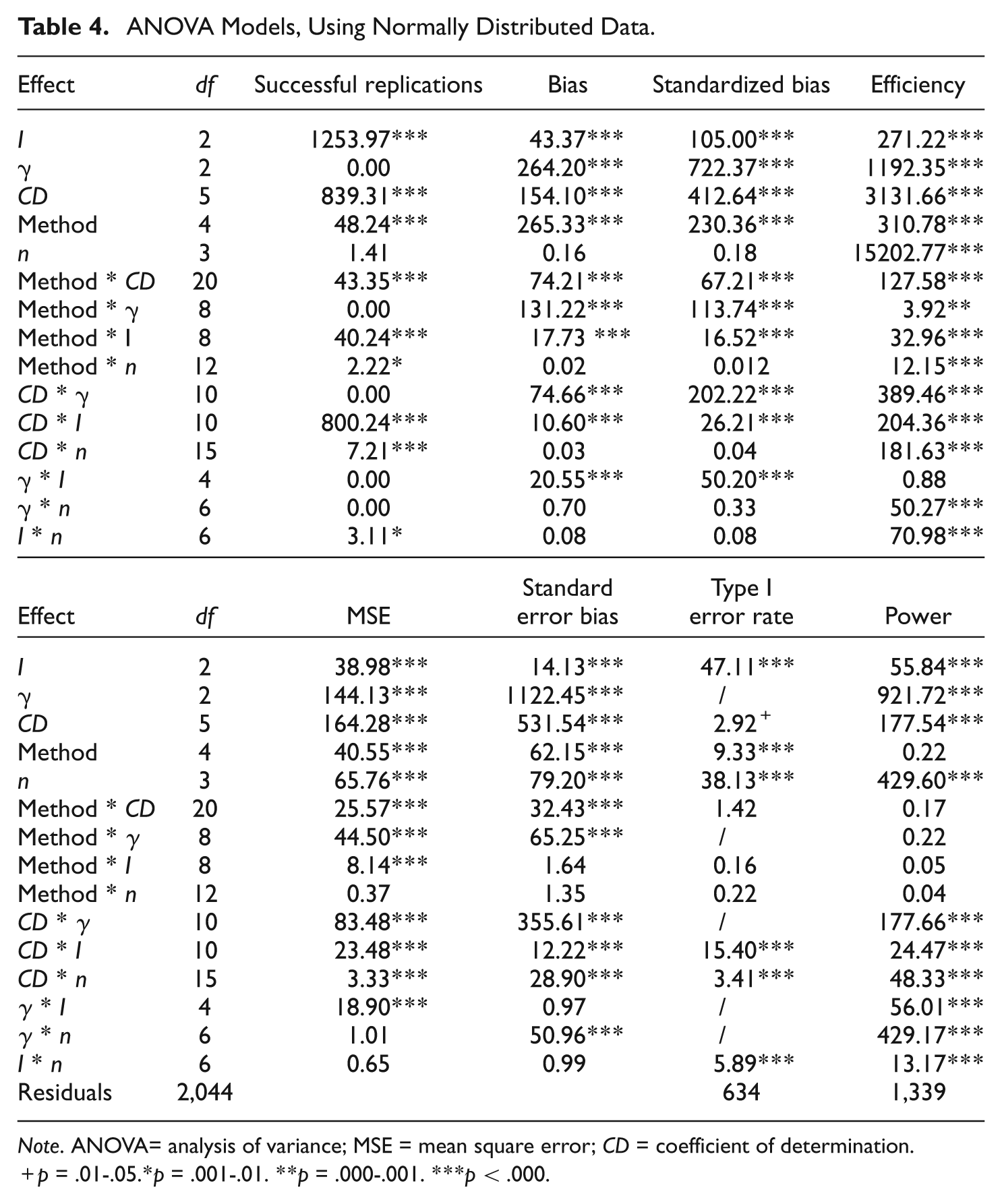
Note. ANOVA= analysis of variance; MSE = mean square error; CD = coefficient of determination.

p = .01-.05.*p = .001-.01. **p = .000-.001. ***p < .000.

Study 2

The same ANOVAs were performed when the data were not normally distributed. However, one extra independent variable was added, namely the degree of nonnormality. This resulted in 21 predictors. The results can be found in Table 6.

Results of Study 1

The results are discussed per statistical performance criterion. The proportion of successful replications, the bias, and efficiency results are discussed first, followed by the MSE, standard error bias, type I error rate, and power. In Table 5, a comparison between the methods for all performance criteria is given.

Table 5.

Comparison Between the Five Methods per Performance Criteria.

	Regression FSR	Bartlett FSR	Bias avoiding	Bias correcting	SEM
Number of successful replications	2	2	2	2	1
Bias	4	5	1	1	1
Standardized bias	3	3	3	1	1
Efficiency	2	1	3	4	4
MSE	4	5	1	1	1
Standard error bias	4	2	5	3	1
Type I error	1	1	1	1	1
Power	1	1	1	1	1

Note. MSE = mean square error. The numbers indicate the performance of the methods in relation to each other for each performance criteria. A score of 1 means the method performed best on that particular performance criteria, while a score of 5 means the method performed the worst.

Proportion of Successful Replications

The first performance measure that was considered was the proportion of successful replications for each method. The proportion of successful replications is very high for all methods and conditions, namely 0.989 or higher. The proportion of successful replications of SEM is even higher than the proportions of the other four methods, which all have the same proportions.

Bias

As can be seen in Figure 3A, only the regression FSR and the Bartlett FSR method are biased, whereas the three remaining methods are not. More specifically, both methods underestimate the regression coefficient and the Bartlett FSR method is more severely biased than the regression FSR method. Moreover, the bias is not influenced by the sample size, implying that both the regression and Bartlett FSR methods are also inconsistent. The bias does disappear with an increasing factor loading and when γ is equal to 0. When the number of items goes up, the bias also declines, but has not disappeared completely when the number of items reaches 10. The three other methods, namely the bias avoiding, bias correcting, and SEM method, exhibit, as expected, very little bias. The three methods perform very similar.

Figure 3.

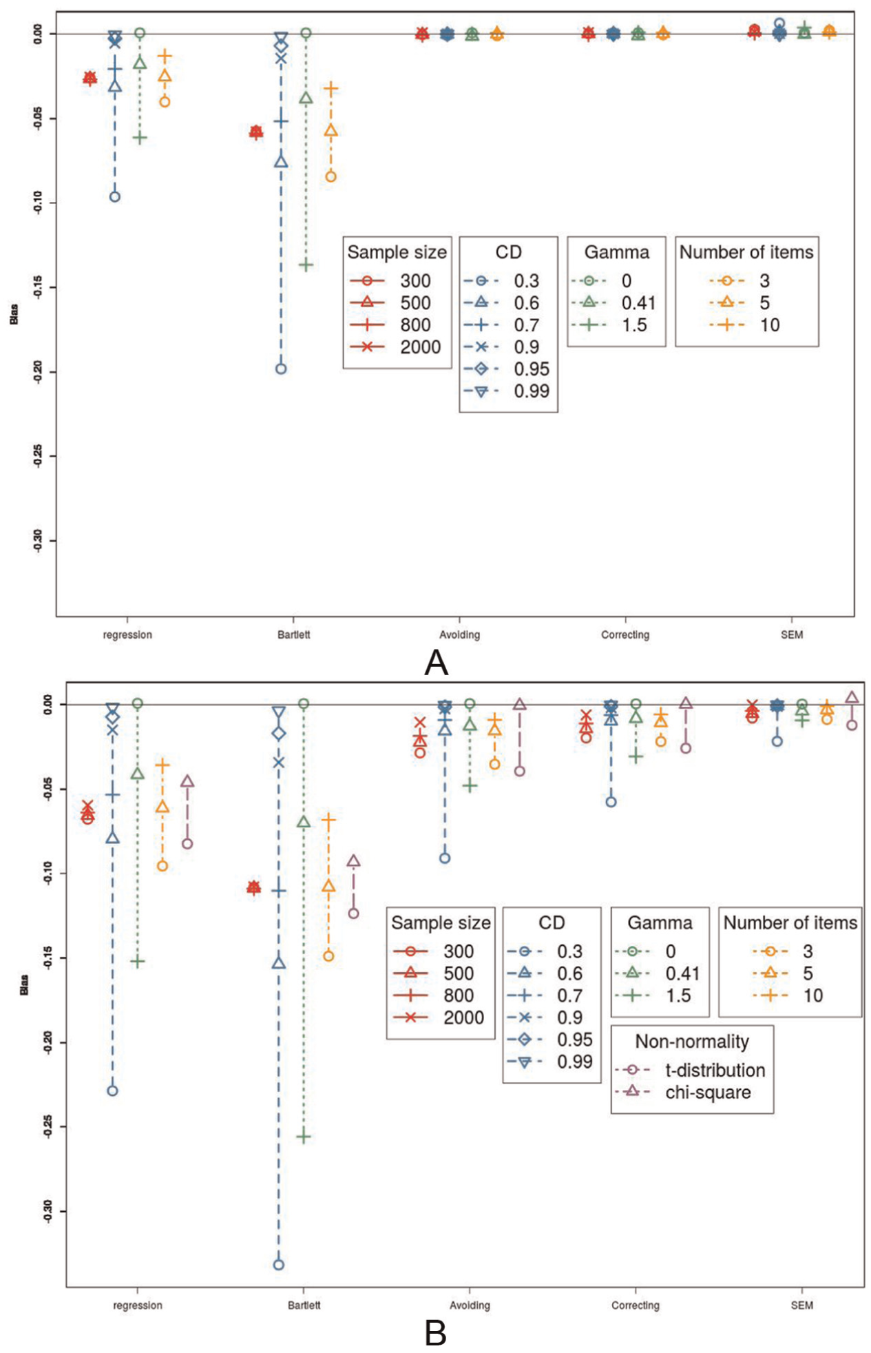
Bias. (A) The influence of sample size, coefficients of determination (CD), number of items, and the value of γ on the bias, in interaction with the method. (B) The influence of sample size, coefficient of determination, number of items, and the value of γ on the bias, in interaction with the method, when the data are not normally distributed.

Bias Using Standardized Parameterization

The patterns change slightly when the standardized parameterization is used (see Figure 4A). Now, the bias avoiding method also underestimates the regression coefficient and is inconsistent. There is also no longer a difference between the Bartlett FSR, regression FSR, and bias avoiding methods. All other effects can be interpreted in the same way as in the unstandardized parameterization.

Figure 4.

Bias using the standardized parameterization. (A) The influence of sample size, coefficients of determination (CD), number of items, and the value of γ on the bias using the standardized parameterization, in interaction with the method. (B) The influence of sample size, coefficients of determination (CD), number of items, and the value of γ on the bias using the standardized parameterization, in interaction with the method, in interaction with the method, when the data are not normally distributed.

Efficiency

While regression FSR and Bartlett FSR are the most biased methods, they are also the most efficient methods. The Bartlett FSR method is even slightly more efficient than the regression FSR method. The three other methods have very similar standard errors. However, the bias avoiding method is slightly more efficient than the other two when the coefficient of determination is low. It is also important to note that the differences between the methods disappear as the coefficient of determination increases.

Mean Square Error

The regression and Bartlett FSR methods have a high MSE, as compared with the other three methods, with the Bartlett FSR having the worst MSE. The MSE of the other three methods is very similar to each other. The differences between the five methods disappear when the CD approaches 1 or when the value of γ approaches 0.

Standard Error Bias

With regard to the standard error bias, there is a large difference between the methods. In Figure 5A, it can be seen that all five methods show bias in the standard error. However, the SEM method clearly has the smallest standard error bias. The four alternative methods are more severely biased with regard to the standard error. On average, the Bartlett FSR method gives the second best estimation of the standard error, followed by the bias correcting and regression FSR methods.

Figure 5.

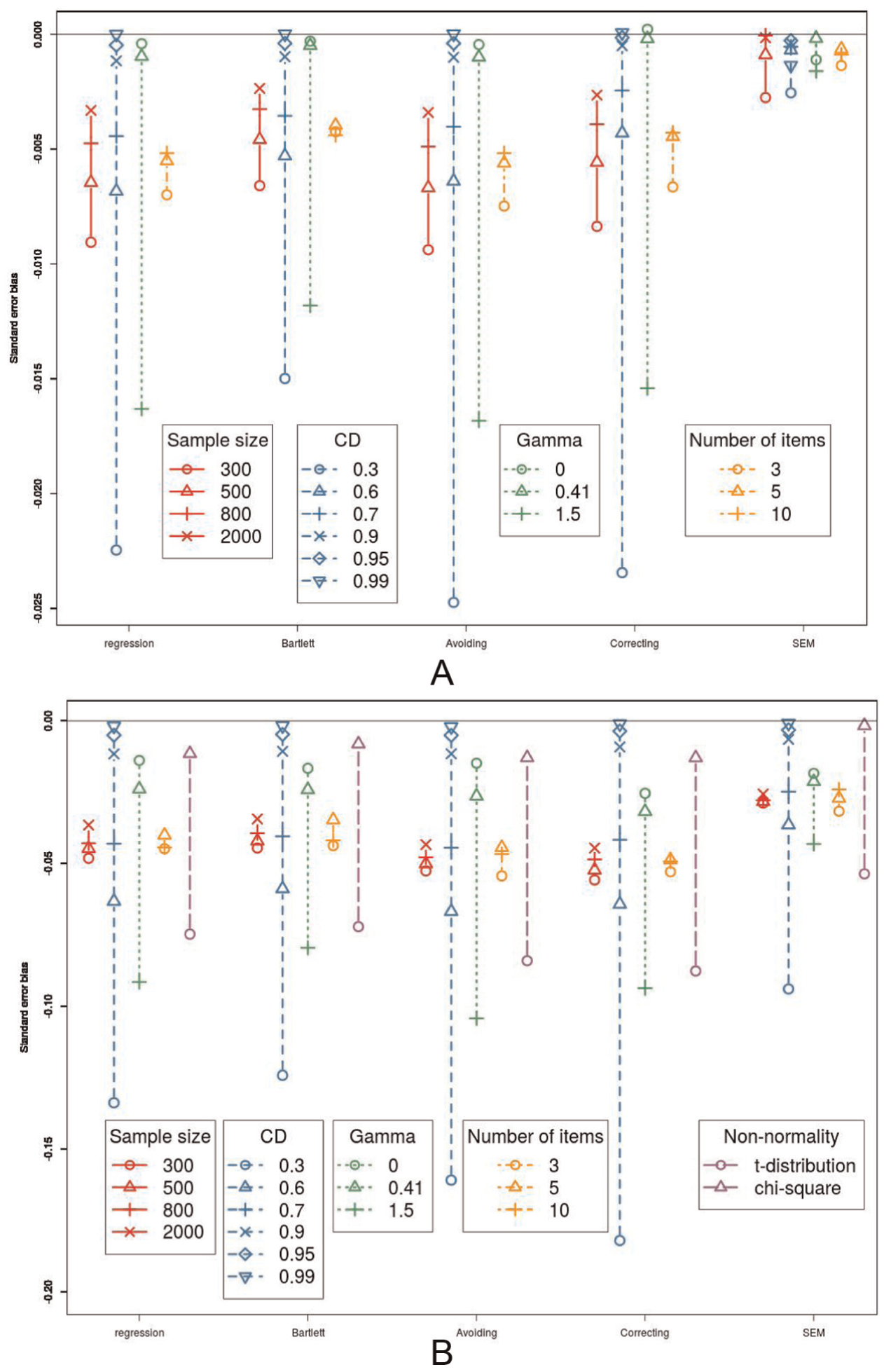
Standard error bias. (A) The influence of sample size, coefficients of determination, number of items, and the value of γ on the standard error bias, in interaction with the method. (B) The influence of sample size, coefficients of determination, number of items, and the value of γ on the standard error bias, in interaction with the method, in interaction with the method, when the data are not normally distributed. Note that the scale of the y-axis is not the same as in (A).

Over all methods, a higher sample size, a higher CD or more items, lowers the standard error bias, while a larger value of γ increases the standard error bias. When the CD approaches 1, all differences between the methods disappear and when the value of γ increases, the differences between the methods also increases. It is important to note that when there is no effect ( $γ = 0$ ), the standard error bias almost completely disappears for all five methods. This means the standard error bias will have little effect on the type I error rate.

Type I Error

The type I error rates for the regression FSR, Bartlett FSR and bias avoiding method are very similar, while SEM has a slightly higher type I error rate and the bias correcting method has a slightly lower type I error rate. While these differences are statistically significant, for all five methods the type I error rates are around the expected value of 0.05. In practice, this means these differences are not really relevant.

Power

All five methods have approximately the same power. There are only small differences when the coefficient of determination is very weak. In that case, SEM has the lowest power, followed by the bias correcting method. The other methods have the same power.

Results of Study 2

The results of the second study are described in relation to the first study. The impact of the kind of nonnormality is also discussed.

Proportion of Successful Replications

When the data are not normally distributed, the proportion of successful replications is a lot lower and the differences between the methods are larger. Especially the proportion of successful replications of SEM is very low as compared with the other four methods. This is mostly due to the conditions where the coefficient of determination is very low (CD = 0.3) or the number of items is low (I = 3). The proportion of the bias correcting method is the second lowest, followed by the bias avoiding method. The regression FSR method has the highest proportion of successful replications. All these effects are largely due to the conditions where a t-distribution was used to simulate the item responses. The χ² distribution seems to have less effect. This could be due to the fact that the kurtosis is larger when using the t-distribution than when using the χ² distribution.

Bias

With regard to the bias, there are two main shifts in the patterns (Figure 3B). First, now, there is a difference between SEM, the bias avoiding, and bias correcting methods. SEM still shows almost no bias, while the bias correcting and bias avoiding methods do show a little bias. The bias avoiding method is more biased than the bias correcting method. The regression FSR and Bartlett FSR still show a large amount of bias. Second, the sample size does have an influence for SEM, the bias avoiding, and bias correcting method. Because of the larger bias in these methods, it can now be seen that these methods are consistent. Again, these patterns are largely caused by the conditions using the t-distribution.

Bias Using Standardized Parameterization

The patterns with regard to the bias using standardized parameterization change in two ways (see Figure 4B). First, both SEM and the bias correcting method show a small bias in the standardized regression parameter, with SEM having the smallest bias. Second, the sample size does have an influence on the bias of the bias correcting and SEM method when the data are not normally distributed. When the sample size increases, the bias decreases.

Efficiency

The efficiency is a lot lower when the data are not normal, especially when the t-distribution was used to simulate the data.

Mean Square Error

While the MSE of SEM, bias correcting, and bias avoiding method were very similar to each other when the data were normally distributed, now there are small differences. SEM has the smallest MSE, closely followed by the bias correcting method. This is again due to the high kurtosis of the conditions simulated with the t-distribution. All other effects remain the same.

Standard Error Bias

When the data are not normally distributed, the standard error bias of the bias correcting method is the worst in some conditions (see Figure 5B), especially when the CD or the value of γ is very low.

Type I Error

When the data are not normally distributed, especially when there is a high kurtosis, the type I error rate is larger than the expected value of 0.05 for all methods. Especially the bias correcting method seems to have a large type I error rate, when the coefficient of determination is very low, namely CD = 0.30.

Power

As can be expected, the power seems to be lower when the data are not normally distributed. Table 6 shows that the method does not have a significant influence on the power, when the data are not normally distributed.

Table 6.

ANOVA Models, Using Nonnormal Data.

Effect	df	Successful replications	Bias	Standardized bias	Efficiency
I	2	124.49***	168.59***	270.76***	240.69***
γ	2	0.00	1215.43***	2449.80***	2974.83***
CD	5	1219.83***	686.33***	1266.31***	6770.51***
Method	4	183.97***	528.00***	525.92***	190.16***
n	3	79.03***	4.31*	4.24*	2657.27***
Nonnormality (NN)	1	2100.28***	299.53***	342.32***	8044.76***
Method *CD	20	121.49***	110.43***	122.62***	15.08***
Method *γ	8	0.00	262.68***	264.49***	3.55**
Method *I	8	28.19***	22.15***	25.99***	3.15*
Method *n	12	1.83⁺	0.55	0.20	0.49
Method * NN	4	153.36***	5.82**	7.09***	3.15*
CD*γ	10	0.00	340.41***	615.95***	644.05***
CD*I	10	36.24***	33.25***	45.76***	32.18***
CD*n	15	36.33***	2.64**	1.77	62.45***
CD* NN	5	1087.06***	111.44***	92.32***	1874.78***
γ*I	4	0.00	77.43***	126.66***	4.54*
γ*n	6	0.00	1.88	1.33	2.57⁺
γ* NN	2	0.00	152.23***	165.91***	1060.31***
I*n	6	3.39*	1.07	0.42	4.04**
I* NN	2	61.01***	22.12***	14.55***	8.72**
n* NN	3	54.25***	7.35***	2.89⁺	2.53
Effect	df	MSE	Standard error bias	Type I error rate	Power
I	2	96.50***	4.57⁺	3.83⁺	321.30***
γ	2	824.44***	2473.21***	/	3549.41***
CD	5	935.59***	2733.13***	378.18***	1307.85***
Method	4	48.17***	95.91***	35.50***	0.72
n	3	70.00***	4.67*	31.634***	810.00***
Nonnormality (NN)	1	657.45***	6300.45***	1804.36***	365.06***
Method *CD	20	20.40***	35.43***	31.72***	1.49
Method *γ	8	64.50***	70.14***	/	0.99
Method *I	8	3.88**	2.19⁺	1.27	0.57
Method *n	12	0.48	0.68	1.21	0.05
Method * NN	4	5.28**	22.85***	33.79***	2.11
CD*γ	10	408.33***	524.64***	/	926.40***
CD* I	10	38.39***	0.74	15.70***	111.62***
CD*n	15	16.93***	1.48	17.76***	114.89***
CD* NN	5	308.80***	1449.50***	340.35***	126.93
γ*I	4	55.55***	23.48***	/	198.07***
γ*n	6	4.79	9.81***	/	662.82***
γ* NN	2	265.38***	1037.45***	/	158.74***
I*n	6	1.13	0.64	1.36	22.92***
I* NN	2	3.88**	8.01**	0.31	26.26***
n* NN	3	11.56***	0.71	74.15***	13.08
Residuals	4,187			1,339	2,763

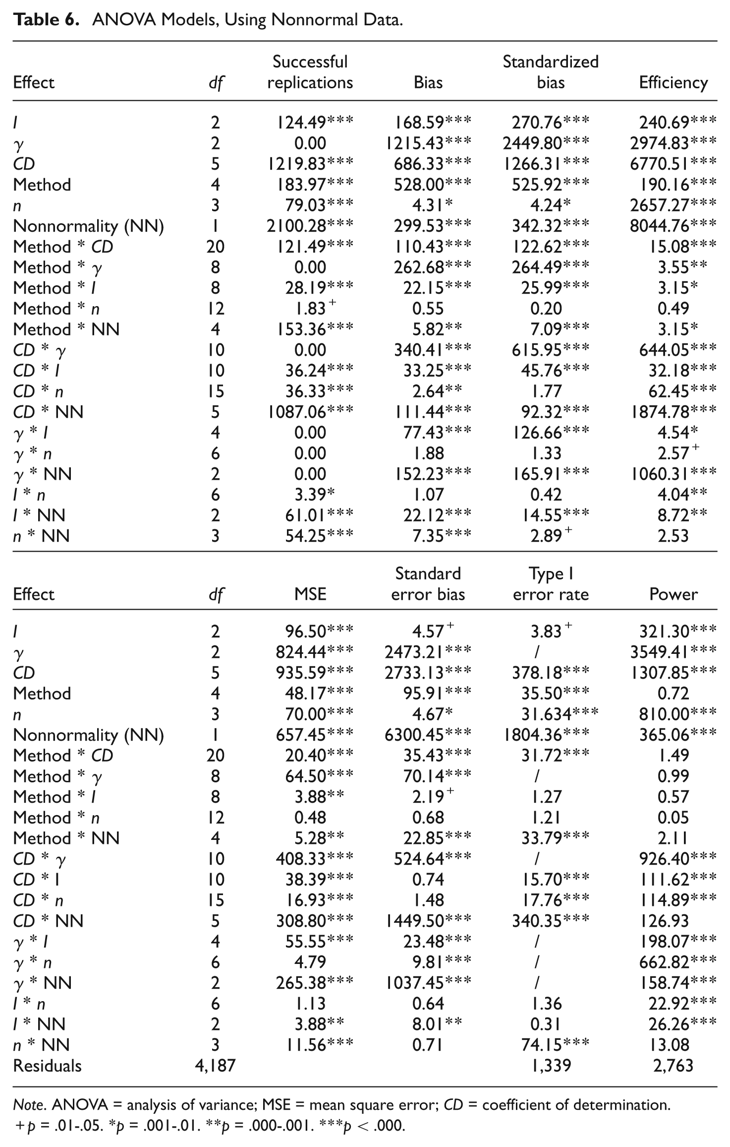
Note. ANOVA = analysis of variance; MSE = mean square error; CD = coefficient of determination.

p = .01-.05. *p = .001-.01. **p = .000-.001. ***p < .000.

Discussion

In this article, an overview was given of four methods for FSR, namely regression FSR, Bartlett FSR, the bias avoiding method (Skrondal & Laake, 2001), and the bias correcting method (Croon, 2002). The four methods were described and their statistical properties were discussed on the population level. Since there was no adequate standard error available for the bias correcting method, a new standard error was developed. To be able to determine the statistical properties of the methods in finite samples and to evaluate the performance of the newly developed standard error, two Monte Carlo simulation studies were performed.

The simulation studies showed that the regression FSR method does not perform well. This confirms the general expectations found in the literature (e.g., Bollen, 1989; Croon, 2002; Lastovicka & Thamodaran, 1991; Lewis & Linzer, 2005; Shevlin et al., 1997; Skrondal & Laake, 2001). It also complies with the results of Lu et al. (2011). The method is biased for both the standardized and unstandardized parameterization and is inconsistent. The method does have a high efficiency, but it also has a high MSE. This means that the high efficiency cannot compensate for the high bias. Moreover, the estimates of the standard error have the second highest bias observed.

The Bartlett FSR method performs even worse than the regression FSR method, with a comparable bias using the standardized parameterization, but a higher unstandardized bias and MSE. It does have a lower standard error bias. It is also the most efficient method, but at the same time it has the highest bias and MSE of all methods.

The first corrected method, namely the bias avoiding method of Skrondal and Laake (2001), only performs slightly better than the regression FSR and Bartlett FSR methods. It is unbiased when using the unstandardized parameterization, but it is still biased when using the standardized parameterization. This result highlights the fact that standardized and unstandardized regression coefficients do not always behave in the same way (Kim & Mueller, 1976). The standard error bias is the largest of all methods and it has the same power and type I error rate as regression FSR and Bartlett FSR. It can be concluded that this method only outperforms regression FSR and Bartlett FSR with regard to the unstandardized bias and is outperformed by SEM and the bias correcting method.

The second corrected method, the bias correcting method, performs better than the bias avoiding method. It is unbiased for both the standardized and unstandardized parameterization and has the highest power. When the observed item responses are not normally distributed, it does show a slightly larger bias than the SEM method, but its proportion of successful replications is also much higher. With regard to the standard error bias, only SEM and Bartlett FSR do better. This result shows that the newly developed standard error is reliable and even performs better than the regular standard error used in the bias avoiding method. However, it is important to note that when the data are not normally distributed and the factor loadings are very weak (CD = 0.3), the standard error bias goes up, resulting in a higher type I error rate. In all other conditions, the estimate of the standard error is reliable. The method not only has the lowest efficiency but also has the lowest MSE, meaning that the low efficiency does not have much influence.

The SEM method performs very similar to the bias correcting method. When the data are normally distributed, SEM has the same bias when using the unstandardized and standardized parameterization, efficiency, MSE, power, and type I error rate. When the data are not normally distributed, SEM not only has a lower bias and MSE but also has a very low proportion of successful replications. This means that, although SEM gives less biased regression coefficients, the chance that the model will not converge, is also much larger for SEM. On the other hand, there is almost no standard error bias when using the SEM method.

Overall, it can be concluded that only the bias correcting method is a suitable alternative for SEM. The method performs similar to the SEM method with regard to bias, efficiency, MSE, power, and type I error rate. It does have more standard error bias than SEM, but it has the second lowest standard error bias of the four FSR methods. It also has more successful replications than SEM when the data are not normally distributed. The method does have some drawbacks in comparison with SEM, because of its two-step nature. First, at this moment, there are no overall fit indices available. Second, the method cannot be used for all possible structural models. For example, the method cannot handle mediational relationships and is not applicable to nonrecursive methods. However, it is the intention of the authors to extend the method to be applicable to the full SEM model and to develop a set of fit indices for this method.

A second conclusion that can be made is that factor score indeterminacy plays a great role in deciding which method to use. The simulation study showed that if the factor score indeterminacy is low (i.e., a CD of 0.99) the differences between the methods disappear completely, on all performance criteria. As a result, there is no longer a problem with performing a conventional FSR. This implies that it is important to first determine the factor score indeterminacies by use of indeterminacy indices. If these indices suggest that the indeterminacies are very low, any of the methods can be used. If these indices suggest the indeterminacies are moderate or high, one should use SEM or the bias correcting method.

In this article it was shown that the bias correcting method of Croon (2002) is a reliable and unbiased method to perform a FSR. A new and reliable standard error was also developed, meaning that the bias correcting method can now be used by applied users to perform significance tests. However, performing the method is a rather complex and technical process. For this reason, software to perform the method will be developed and made available for the applied users in the near future.

Footnotes

Appendix A

Appendix B

Appendix C

Appendix D

Appendix E

Declaration of Conflicting Interests

The author(s) declared no potential conflicts of interest with respect to the research, authorship, and/or publication of this article.

Funding

The author(s) received no financial support for the research, authorship, and/or publication of this article.

References

Acito

Anderson

R. D.

(1986). A simulation study of factor score indeterminacy. Journal of Marketing Research, 23, 111-118. doi:10.2307/3151658

Bartlett

M. S.

(1937, July). The statistical conception of mental factors. British Journal of Psychology: General Section, 28, 97-104. doi:10.1111/j.2044-8295.1937.tb00863.x

Bentler

P. M.

Chou

C.-P.

(1987). Practical issues in structural modeling. Sociological Methods & Research, 16, 78-117. doi:10.1177/0049124187016001004

Bollen

(1989). Structural equations with latent variables. New York, NY: Wiley.

Bollen

Hoyle

R. H.

(2012). Latent variables in structural equation modeling. In Hoyle

R. H.

(Ed.), Handbook of structural equation modeling (pp. 59-67). New York, NY: Guilford Press.

Croon

(2002). Using predicted latent scores in general latent structure models. In Marcoulides

Moustaki

(Eds.), Latent variable and latent structure modeling (pp. 195-223). Mahwah, NJ: Lawrence Erlbaum.

Grice

J. W.

(2001). Computing and evaluating factor scores. Psychological Methods, 6, 430-450. doi:10.1037//1082-989X.6.4.430

Jöreskog

K. G.

(1973). A general method for estimating a linear structural equation system. In Goldberger

Duncan

(Eds.), Structural equation models in the social sciences (pp. 85-112). New York, NY: Seminar Press. doi:10.1002/j.2333-8504.1970.tb00783.x

Kim

J.-O.

Mueller

C. W.

(1976). Standardized and unstandardized coefficients in causal analysis: An expository note. Sociological Methods & Research, 4, 423-438. doi:10.1177/004912417600400402

10.

Lastovicka

J. L.

Thamodaran

(1991). Common factor score estimates in multiple regression problems. Journal of Marketing Research, 28, 105-112. doi:10.2307/3172730

11.

Lewis

J. B.

Linzer

D. A.

(2005). Estimating regression models in which the dependent variable is based on estimates. Political Analysis, 13, 345-364. doi:10.1093/pan/mpi026

12.

I. R.

Kwan

Thomas

D. R.

Cedzynski

(2011). Two new methods for estimating structural equation models: An illustration and a comparison with two established methods. International Journal of Research in Marketing, 28, 258-268. doi:10.1016/j.ijresmar.2011.03.006

13.

I. R.

Thomas

D. R.

(2008). Avoiding and correcting bias in score-based latent variable regression with discrete manifest items. Structural Equation Modeling, 15, 462-490. doi:10.1080/10705510802154323

14.

I. R.

Thomas

D. R.

Zumbo

B. D.

(2005). Embedding IRT in structural equation models: A comparison with regression based on IRT scores. Structural Equation Modeling, 12, 263-277. doi:10.1207/s15328007sem1202

15.

Maraun

M. D.

(1996). Metaphor taken as math: Indeterminancy in the factor analysis model. Multivariate Behavioral Research, 31, 517-538. doi:10.1207/s15327906mbr3104_6

16.

Mulaik

S. A.

(1972). Factor scores and factor indeterminacy. In Mulaik

S. A.

(Ed.), Foundations of factor analysis. New York, NY: McGraw-Hill.

17.

R Development Core Team. (2008). R: A language and environment for statistical computing. Vienna, Austria: R Foundation for Statistical Computing.

18.

Shevlin

Miles

Bunting

(1997). Summated rating scales. A Monte Carlo investigation of the effects of reliability and collinearity in regression models. Personality and Individual Differences, 23, 665-676. doi:10.1016/S0191-8869(97)00088-3

19.

Skrondal

Laake

(2001). Regression among factor scores. Psychometrika, 66, 563-575. doi:10.1007/BF02296196

20.

Skrondal

Rabe-Hesketh

(2004). Generalized latent variable modeling: Multilevel, longitudinal and structural equation models. Boca Raton, FL: Chapman & Hall/CRC Press.

21.

Steiger

J. H.

(1979). Factor indeterminacy in the 1930’s and the 1970’s some interesting parallels. Psychometrika, 44, 157-167. doi:10.1007/BF02293967

22.

Thomson

G. H.

(1934). The meaning of “i” in the estimate of “g”. British Journal of Psychology, 25, 92-99. doi:10.1111/j.2044-8295.1934.tb00728.x

23.

Thomson

G. H.

(1938). Methods of estimating mental factors. Nature, 141, 246-246. doi:10.1038/141246a0

24.

Thurstone

(1935). The vectors of mind. Chicago, IL: University of Chicago Press.