On the Fallibility of Principal Components in Research

Abstract

The measurement error in principal components extracted from a set of fallible measures is discussed and evaluated. It is shown that as long as one or more measures in a given set of observed variables contains error of measurement, so also does any principal component obtained from the set. The error variance in any principal component is shown to be (a) bounded from below by the smallest error variance in a variable from the analyzed set and (b) bounded from above by the largest error variance in a variable from that set. In the case of a unidimensional set of analyzed measures, it is pointed out that the reliability and criterion validity of any principal component are bounded from above by these respective coefficients of the optimal linear combination with maximal reliability and criterion validity (for a criterion unrelated to the error terms in the individual measures). The discussed psychometric features of principal components are illustrated on a numerical data set.

Keywords

criterion validity error variance measurement error principal component principal component analysis reliability validity

Principal component analysis (PCA) is a widely used multivariate statistical technique for data reduction in the behavioral, biological, business, educational, engineering, medical, social, and natural sciences (e.g., Raykov & Marcoulides, 2008). The PCA feature that is particularly appealing to empirical scientists is its variance optimization property. This feature is associated with the individual principal components (PCs), which are typically extracted from a given set of observed measures following traditionally used selection criteria (e.g., Johnson & Wichern, 2002) and possibly some associated interval estimation procedures (e.g., Raykov & Marcoulides, 2014; see also Härdle & Hlavka, 2007). A consequential misinterpretation of this optimality property that is frequently encountered in the extant literature, however, in particular with respect to the first PC, is that this feature somehow deals away with any potential error variance inherent in the observed variables, or at least reduces it to an effectively negligible extent. A related misleading interpretation can be similarly found for instance in some missing data analysis literature, which could be taken to imply that the PCs extract entirely reliable variance from the analyzed measure set and that especially the first PC is completely reliable (i.e., error-free). Given the widespread utilizations of PCA, particularly for purposes of addressing measurement related problems, it is essential that such myths are dispelled. The aim of this note is to contribute to this process by providing a discussion highlighting the error-prone nature of PCs and evaluating the impact that measurement error has on any PC extracted from a set of observed measures containing at least one error-prone variable.

The plan of the article is as follows. We first review briefly the basic features of PCA, focusing on those of the PCs. In the next section, we show that the error variance in any PC (a) cannot be smaller than the minimal error variance for a measure in an analyzed set of observed variables and (b) cannot be larger than the maximal error variance for a measure in that set. From these features it follows that any PC, in particular the first extracted PC, cannot have perfect reliability (in case of at least one fallible observed variable). We next point out that if the analyzed set of manifest variables is unidimensional (homogeneous), then any PC cannot have reliability that is larger than that associated with the optimal linear combination of these measures, which is the maximal reliability coefficient. Similarly, we point out that the criterion validity then of any PC cannot be higher than the criterion validity of the same optimal linear combination for any criterion uncorrelated with the error terms in the measures. We illustrate subsequently these developments on numerical data, and we conclude by highlighting the demonstrated limitations of principal components in relation to their psychometric features.

Background, Notation, and Assumptions

In the remainder of this note, we assume that a set of observed measures is given, whereby at least one of these manifest variables contains measurement error as will often be the case in most empirical settings in educational and psychological research. Let these measures be denoted X₁, . . . , X_k (k > 1) and their set by Ξ, that is, Ξ = {X₁, . . . , X_k}. For each of these measures, their classical test theory decomposition exists (in empirical research)—that is, X_j = T_j+e_j holds, where T_j and e_j are its true and error score, respectively (e.g., Raykov & Marcoulides, 2011). We assume that the error terms associated with different observed measures are uncorrelated. (Implications of this assumption are testable; e.g., Raykov, Marcoulides, & Li, 2016.) Whenever a measure is error-free, e_j = 0 holds, while otherwise its error variance is positive (j = 1, . . . , p).¹ In the rest of this discussion, we assume that the latter is true for at least one measure in Ξ—that is, there is at least one error-prone observed variable in a given set of manifest measures that are subjected to a PCA. (Without loss of generality, we can assume that X₁ is fallible; i.e., denoting by ${σ^{2}}_{e_{1}}$ its error variance, ${σ^{2}}_{e_{1}} > 0$ is assumed to hold.)

In PCA, linear combinations Y₁, . . . , Y_k of the original measures in Ξ are sought with the property that the first one, that is, Y₁, maximizes observed variance, that is, has highest variance among all linear combinations of X₁, . . . , X_k. In addition, the PCs Y₂, . . . , Y_k have the property that they minimize the remaining variance in the set of X₁, . . . , X_k under the condition that each PC is uncorrelated with all preceding PCs extracted before it, that is, Y_j is uncorrelated with Y₁, . . . , Y_j_{− 1} (2 ≤j≤k; e.g., Timm, 2002). We assume in the remainder that the covariance matrix of X₁, . . . , X_k, denoted ∑, is positive definite and is subjected to a PCA. (Conducting a PCA on the correlation matrix does not alter the developments, findings, and interpretations in the rest of this discussion; e.g., Joliffe, 2002.) Last but not least, we note that unless stated otherwise, the rest of this article evolves at the population level, that is, any quantity appearing below will be taken to be a population quantity, unless indicated otherwise (in particular, in the Illustration section).

As is well known, the weights in the linear combinations of X₁, . . . , X_k that render each of the PCs are the consecutive elements of the normalized eigenvectors pertaining to the successive eigenvalues (e.g., Raykov & Marcoulides, 2008). Placing these eigenvectors correspondingly as columns in the matrix P = [p_ij], and their pertinent eigenvalues as successive main diagonal elements of the diagonal Matrix Λ, the following decomposition holds thereby (e.g., Timm, 2002):

Σ = P Λ P',

with the matrix P being orthogonal, that is, P P′ = P′ P = I_k, where I_k is the k×k identity matrix (priming denotes transposition in this article). The orthogonality feature of P will play an important role in the remainder.

Error Variance in a Principal Component

Suppose one selected the jth PC, Y_j, for further consideration (1 ≤j≤k). From the earlier discussion in this article, this component is the following linear combination of the initial set Ξ of observed measures:

Y_{j} = p_{1 j} X_{1} + p_{2 j} X_{2 j} + \dots + p_{kj} X_{kj},

where the abovementioned orthogonality property of P entails the following equality (specifically following from P′ P = I_k):

{p_{1 j}}^{2} + {p_{2 j}}^{2} + \dots + {p_{kj}}^{2} = 1,

which will prove instrumental in the rest of this section.

To address the potential error-proneness of PCs, let ${σ^{2}}_{e, min}$ and ${σ^{2}}_{e, max}$ be the smallest and largest error variance, respectively, associated with an observed measure in the set Ξ. (If only one of the observed measures is fallible while all remaining k− 1 are error-free, then ${σ^{2}}_{e, min}$ and ${σ^{2}}_{e, max}$ equal each the error variance in that manifest variable.) Evidently, ${σ^{2}}_{e, min}$ and ${σ^{2}}_{e, max}$ are both positive, due to the earlier made assumption of at least one measure in Ξ being fallible.

With the preceding in mind, from the last section it obviously follows that (cf., e.g., Raykov & Marcoulides, 2011)

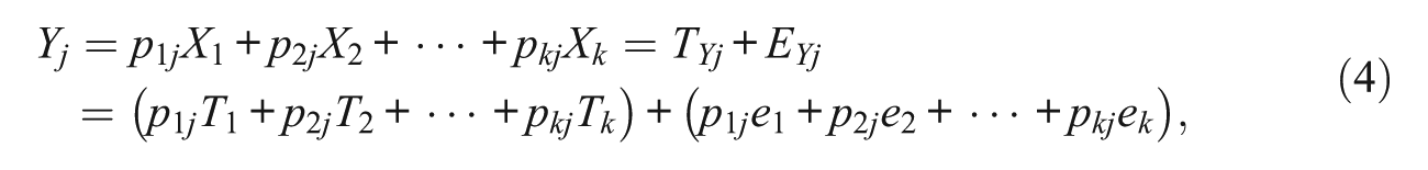
\begin{matrix} Y_{j} = p_{1 j} X_{1} + p_{2 j} X_{2} + \dots + p_{kj} X_{k} = T_{Yj} + E_{Yj} \\ = (p_{1 j} T_{1} + p_{2 j} T_{2} + \dots + p_{kj} T_{k}) + (p_{1 j} e_{1} + p_{2 j} e_{2} + \dots + p_{kj} e_{k}), \end{matrix}

that is, the first and second terms in brackets in the right-hand side of Equation (4) represent the true and error scores, respectively, of the jth PC, which are correspondingly denoted T_Yj and E_Yj (j = 1, . . . , k).

From Equation (4) it is readily seen that Y_j will be error-free if and only if the second term in parentheses in its (last) right-hand side vanishes (j = 1, . . . , k). In particular, Y_j will possess “perfectly reliable” variance (i.e., will contain no error variance), if and only if the variance of its error term E_Yj is 0, that is, if and only if the variance of p₁ _je₁+p₂ _je₂+···+p_kje_k is 0. It can also be noted from Equation (4) that the amount of error variance in the jth PC depends to a considerable degree on that in the variables that receive the largest weights in the linear combination rendering that PC (the right-hand side of (4); j = 1, . . . , k). This relation will obviously be more pronounced if larger weights go with observed variables having more measurement error (i.e., contain larger error variances).

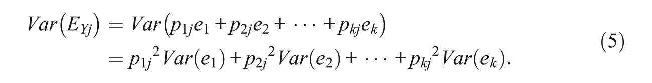
With Equation (4) in mind, simple algebra shows that for the error variance in Y_j evidently the following equation holds (where Var(.) denotes variance; recall also the assumption of uncorrelated error scores in the observed measures):

\begin{array}{l} V a r (E_{Y j}) = V a r (p_{1 j} e_{1} + p_{2 j} e_{2} + \dots + p_{k j} e_{k}) \\ = {p_{1 j}}^{2} V a r (e_{1}) + {p_{2 j}}^{2} V a r (e_{2}) + \dots + {p_{k j}}^{2} V a r (e_{k}) . \end{array}

Since $Var (e_{j}) \geq {σ^{2}}_{e, min}$ , Equations (3) and (5) entail for each j = 1, . . . , k, that is, for each PC,

\begin{matrix} Var (E_{Yj}) = {p_{1 j}}^{2} Var (e_{1}) + {p_{2 j}}^{2} Var (e_{2}) + \dots + {p_{kj}}^{2} Var (e_{k}) \\ \geq {σ^{2}}_{e, min} ({p_{1 j}}^{2} + {p_{2 j}}^{2} + \dots + {p_{kj}}^{2}) \\ = {σ^{2}}_{e, min} . \end{matrix}

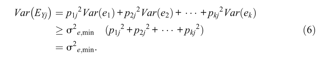
Therefore, if at least one in an analyzed set of observed measures contains measurement error, as assumed in this note, so does also any extracted principal component, and in particular the first principal component. Thereby, the error variance in any PC is at least as large as the smallest error variance associated with an observed measure in that variable set. In other words, PCA does not ‘deal away’ with error variance, as sometimes claimed, implied, or interpreted incorrectly. Specifically, each PC—including in particular the first PC—is error-prone, in fact at least as much as the least error-prone of the analyzed variables. For this reason, as soon as there is a fallible measure in a set of analyzed manifest variables, any PC—and in particular the 1st PC—has reliability that is lower than 1, despite some incorrect statements or interpretations to be found in the literature. Furthermore, and somewhat less formally, no PC—and in particular not the first PC—can “reduce” the error variance beyond the smallest error variance in an error-prone measure from an analyzed data set (see the right-hand side of Inequality 6).

In analogy to the preceding developments it is readily seen that

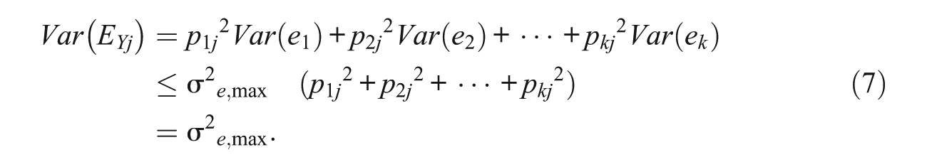
\begin{matrix} Var (E_{Yj}) = {p_{1 j}}^{2} Var (e_{1}) + {p_{2 j}}^{2} Var (e_{2}) + \dots + {p_{kj}}^{2} Var (e_{k}) \\ \leq {σ^{2}}_{e, max} ({p_{1 j}}^{2} + {p_{2 j}}^{2} + \dots + {p_{kj}}^{2}) \\ = {σ^{2}}_{e, max} . \end{matrix}

That is, as long as at least one in an analyzed set of observed measures contains measurement error, the error variance of any PC and in particular of the first PC cannot exceed the largest error variance associated with an observed measure in the set. Put another way, and somewhat less formally, the effect of PCA is the “limitation” of the error variance by that of the measure with maximal error variance in an analyzed set of variables.

From this discussion it follows that any PC is perfectly reliable if and only if all measures in the set are perfectly reliable. In fact, the preceding in this subsection shows that a PC—and in particular the first PC—is perfectly reliable if and only if all measures in the analyzed set are error-free (assuming the measurement error terms, for those that are error-prone, are uncorrelated as mentioned above). In other words, each analyzed measure being perfectly reliable, is a necessary and sufficient condition then for any PC—including in particular the 1st PC—to be perfectly reliable, for a given set of manifest variables involved in a PCA session.

The reason underlying this finding is the fact that by the PCs definition the optimal variance feature of any PC, and in particular of the first PC, is concerned only with observed variance and its “redistribution” from the manifest measures across the PCs. This observed variance optimality feature has no implications, however, in terms of elimination of the error variance contained in one or more of the measures analyzed. Conversely, the perfect reliability feature of a PC, and in particular of the first PC, holds only for analyzed variable sets that consist entirely of error-free measures.

By way of summary, this subsection shows that (as long as measurement errors are uncorrelated) the popular statistical technique of PCA (a) does not remove error variance relative to the smallest error variance in the analyzed data set, and also (b) does not enhance error variance as compared with the largest error variance in the analyzed variables. In simple terms, the error variance in any PC, and in particular in the first PC, cannot be lower than the smallest error variance, and at the same time cannot be higher than the largest error variance of a variable in an analyzed set of observed measures.

Principal Components of Unidimensional Sets of Measures

In some empirical settings, for instance when dealing with auxiliary variables in connection with analysis and modeling of incomplete data sets (e.g., Enders, 2010), a researcher may be concerned with a given unidimensional set, denoted Ω, of observed measures that he or she may be willing to consider first conducting a PCA on (cf. Howard, Rhemtulla, & Little, 2015). The measures in Ω could be for example fallible components of a homogeneous scale that evaluates a construct related to one or more dependent variables with missing data. In such situations, a scholar might become interested in reducing the complexity associated with the multitude of manifest variables in Ω to one or more (but fewer) principal components, and then possibly using the latter as auxiliary variables themselves in the ensuing incomplete data analyses in lieu of that initial set Ω of variables (cf. Howard, 2012). The “temptation” then might be great to consider or even treat these PCs, in particular the first PC, as “perfectly reliable” derived measures resulting from the given set Ω of manifest variables. Such a consideration, treatment, or interpretation however—as pointed out earlier in this section—is incorrect any time at least one component is measured with error and the error terms of the (fallible) scale components are uncorrelated.

In this connection, instead of or in addition to the incorrect interpretation just pointed out, a scholar may be “tempted” to consider or even treat these PCs, in particular the first PC, as possessing another property of special relevance in empirical research. Specifically, based on the above optimality feature of PCs, he or she might incorrectly imply that any PC—in particular the 1st PC—incorporates information from the analyzed scale components rendering it possessing higher validity than what could be achieved with the scale containing the initial set Ω of observed variables. Also this conjecture will be incorrect, as indicated later in the present section.

Reliability of a Principal Component From a Homogeneous Scale

We assume in the remainder of this section that in a given set of unidimensional observed measures none of their loadings on the common factor is 0, none of their error variances are 0 and that these errors are uncorrelated, which represents a setup of relevance in many empirical educational and psychological research settings (e.g., Raykov & Marcoulides, 2011). When the reliability of a PC is then of interest, after a PCA is conducted on this set of measures, we should first remind ourselves that by definition any PC is a linear combination of the observed variables involved. As is well known from the psychometric literature (e.g., Bartholomew, 1996), however, in the setting of concern the so-called optimal linear combination (OLC)

Z = w_{1} X_{1} + w_{2} X_{2} + \dots + w_{k} X_{k},

will be associated with maximal possible reliability across all linear combinations of the involved measures X₁, . . . , X_k. Thereby, these optimal weights (rendering the OLC) are determined as follows:

w_{j} = b_{j} / v_{j},

with b_j being the loading of the jth observed measure on the underlying construct and v_j its error variance (j = 1, . . . , k; e.g., Raykov, 2012). Thereby, the maximal reliability coefficient, that is, the reliability coefficient of the OLC denoted Z in Equation (8), is

ρ^{*} = ({b_{1}}^{2} / v_{1} + \dots + {b_{p}}^{2} / v_{p}) / [1 + ({b_{1}}^{2} / v_{1} + \dots + {b_{p}}^{2} / v_{p})]

(e.g., Bartholomew, 1996). From the right-hand side of (10) it obviously follows then that

ρ^{*} < 1 .

In other words, the maximal reliability of the scale cannot be perfect in the setting under consideration.

With this in mind, since any PC is by definition just a particular linear combination of the elements of the set of analyzed observed variables, X₁, . . . , X_k, it follows that its reliability cannot be higher than the maximal reliability achievable with a linear combination of this set. Therefore, any PC Y_j—and in particular the first PC—has a reliability coefficient, denoted ρ_j, which is no higher than ρ*:

ρ_{j} \leq ρ^{*} (j = 1, \dots, k) .

Inequality (12) shows that the process of PCA cannot render a PC with very (arbitrarily) high reliability, and in particular a PCA will never produce a PC with reliability that is higher than ρ* (in the setting of concern in this section). In other words, PCA cannot purge the error variance from a set of analyzed homogeneous observed measures to an extent that would render any PC—in particular the first PC—having reliability higher than ρ*. Put another way, PCA does not have “unlimited” capability to remove error variance in order to render any PC (and in particular the first PC) as a “purified” measure—for example, of the underlying construct—that would be associated with a reliability higher than the maximal reliability ρ*. (Recall also that as shown earlier in this article, regardless of the relationships among the set of measures analyzed, no PC extracted will have perfect reliability if at least one of the measures is fallible.)

Validity of a Principal Component From a Homogeneous Scale

The limits of PCA with respect to error variance that were highlighted above also extend to validity, in particular to the criterion validity coefficient of a given homogeneous scale with uncorrelated errors. To realize this, we utilize an earlier finding with respect to maximal criterion validity. Specifically, as shown in Penev and Raykov (2006), the criterion validity of the OLC of the homogeneous measures in the above Equation (8) (see also Equations 9) is the maximal among the criterion validity coefficients of all possible linear combinations of the given scale components for any criterion that is uncorrelated with their error terms.

Since any PC is by definition a particular linear combination of the analyzed set of measures, here a set of homogeneous scale components, it follows that its criterion validity cannot be higher than that of the OLC in Equation (8). That is, the process of PCA cannot create a new derived measure in the form of a PC, which would have higher criterion validity than what is achievable with the given set of measures. In other words, any PC—and in particular the first PC—cannot have higher validity than the optimal way in which Equations (8) and (9) utilize the analyzed scale components (at least as far as the predictability of a given criterion is concerned that is uncorrelated with the error terms of the individual components).

It is important to emphasize that the last point is another effective limit that will be beneficial to keep in mind in empirical research when considering applications of PCA.

Illustration on Data

To demonstrate the discussed psychometric limitations of principal components, we utilize a simulated multi-normal data set of n = 1,000 cases for a scale consisting of p = 5 observed variables (components) generated according to the following unidimensional model (congeneric test model; e.g., Jöreskog, 1971):

X_{1} = T + e_{1},

X_{2} = 1.7 T + e_{2},

X_{3} = 1.9 T + e_{3},

X_{4} = 2.2 T + e_{4},

X_{5} = 2.4 T + e_{5},

where T was standard normal and the error terms E₁, . . . , E₅ were zero-mean independent normal variates with variances 1.5, 1.7, 1.4, 1.6, and 1.9, respectively. (Further details on the simulation procedure can be obtained from the authors on request.)

The population covariance matrix associated with this data simulation is readily found to be as follows:

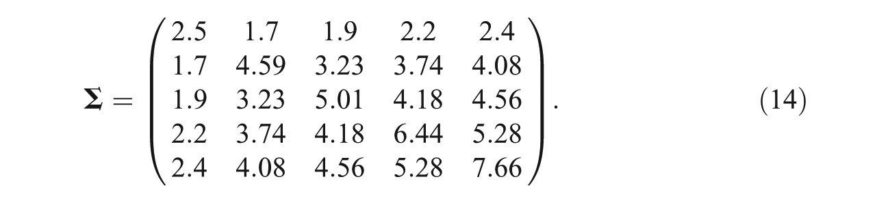
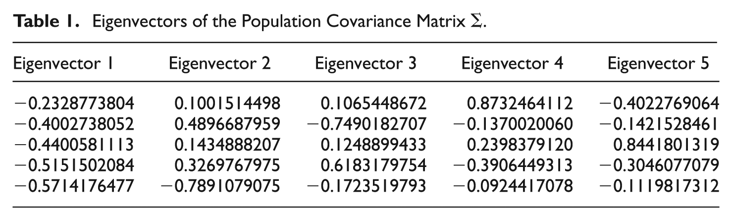
\sum = (\begin{matrix} 2.5 & 1.7 & 1.9 & 2.2 & 2.4 \\ 1.7 & 4.59 & 3.23 & 3.74 & 4.08 \\ 1.9 & 3.23 & 5.01 & 4.18 & 4.56 \\ 2.2 & 3.74 & 4.18 & 6.44 & 5.28 \\ 2.4 & 4.08 & 4.56 & 5.28 & 7.66 \end{matrix}) .

We note that our illustration aims will evidently be achieved when demonstrating the error-proneness of the first PC. (In the same way, however, one can readily proceed with any of the remaining 4 PCs.) With this in mind, a PCA conducted on the covariance matrix in Equation (14) yields the true (population) first PC as follows (weights below are rounded to two decimal places; for full precision, as provided by the used software, see Table 1 and the appendix; SPSS, Inc., 2015):

Y_{1} = - . 23 X_{1} - . 40 X_{2} - . 44 X_{3} - . 52 X_{4} - . 57 X_{5} .

Table 1.

Eigenvectors of the Population Covariance Matrix ∑.

Eigenvector 1	Eigenvector 2	Eigenvector 3	Eigenvector 4	Eigenvector 5
−0.2328773804	0.1001514498	0.1065448672	0.8732464112	−0.4022769064
−0.4002738052	0.4896687959	−0.7490182707	−0.1370020060	−0.1421528461
−0.4400581113	0.1434888207	0.1248899433	0.2398379120	0.8441801319
−0.5151502084	0.3269767975	0.6183179754	−0.3906449313	−0.3046077079
−0.5714176477	−0.7891079075	−0.1723519793	−0.0924417078	−0.1119817312

The error variance in this PC, denoted $Var (E_{Y_{1}}),$ is therefore (see first section of article and above data generating model, specifically with respect to the error variances used in it; asterisk is used in the rest of this section to denote multiplication):

Var (E_{Y_{1}}) = {(- . 23)}^{2}^{*} 1.5 + {(- . 40)}^{2}^{*} 1.7 + {(- . 44)}^{2}^{*} 1.4 + {(- . 52)}^{2}^{*} 1.6 + {(- . 57)}^{2}^{*} 1.9 = 1.67,

which is clearly positive and, no less importantly, of the same (approximate) magnitude as the variances of the original measures X₁ through X₅. Hence, as shown earlier in the article for the general case, the first PC indeed contains positive error variance and is not “perfectly reliable,” that is, the first PC is not error-free. Note that this finding of error-proneness of the first PC is valid already at the population level, that is, when a PCA on the data (covariance matrix) is not at all affected by sampling error.

The covariance matrix of the simulated data set, obtained as described above, is as follows (for simplicity, only its nonredundant elements are presented next):

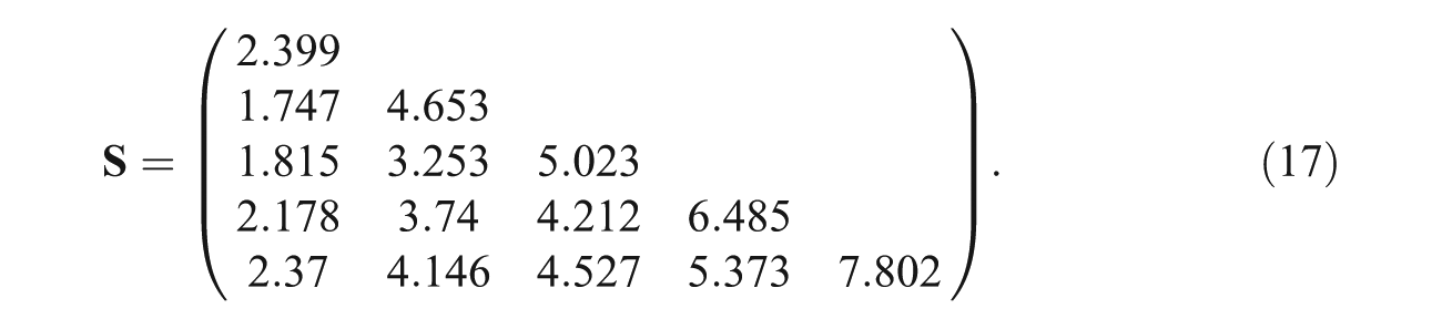
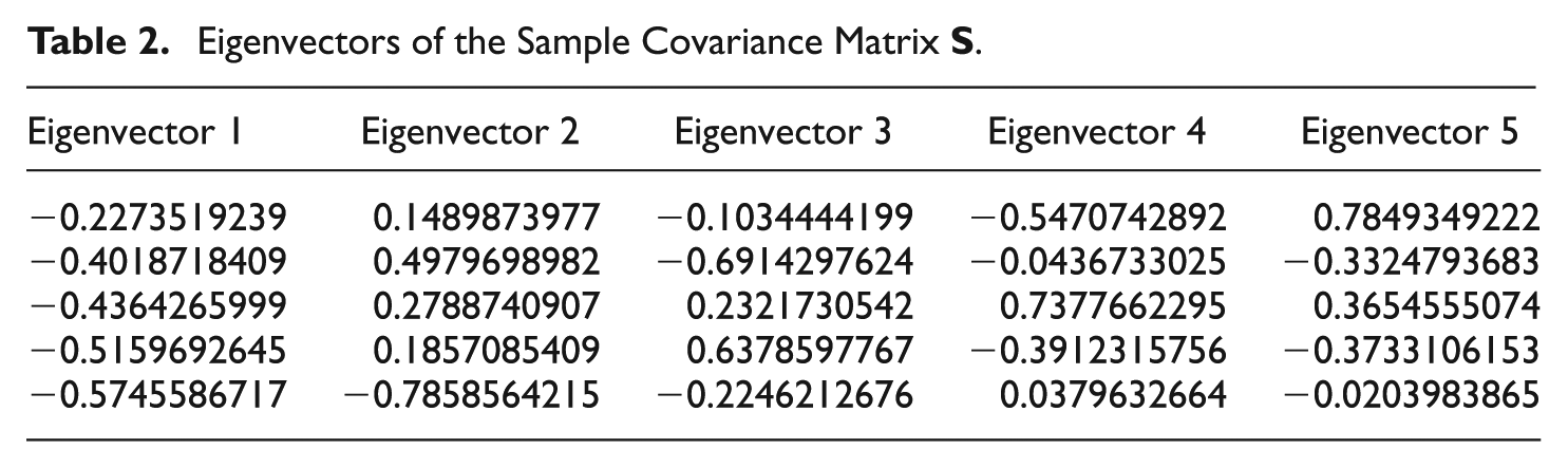
S = (\begin{matrix} 2.399 \\ 1.747 & 4.653 \\ 1.815 & 3.253 & 5.023 \\ 2.178 & 3.74 & 4.212 & 6.485 \\ 2.37 & 4.146 & 4.527 & 5.373 & 7.802 \end{matrix}) .

Conducting a PCA on the empirical covariance Matrix (17) yields the estimated first PC given next (rounded to two decimal places; for full precision, as provided by the used software, see Table 2 and the appendix; hat is used to denote an estimate in the remainder of the article):

{\hat{Y}}_{1} = (- . 23)^{*} X_{1} + (- . 40)^{*} X_{2} + (- . 44)^{*} X_{3} + (- . 52)^{*} X_{4} + (- . 57)^{*} X_{5} .

Table 2.

Eigenvectors of the Sample Covariance Matrix S.

Eigenvector 1	Eigenvector 2	Eigenvector 3	Eigenvector 4	Eigenvector 5
−0.2273519239	0.1489873977	−0.1034444199	−0.5470742892	0.7849349222
−0.4018718409	0.4979698982	−0.6914297624	−0.0436733025	−0.3324793683
−0.4364265999	0.2788740907	0.2321730542	0.7377662295	0.3654555074
−0.5159692645	0.1857085409	0.6378597767	−0.3912315756	−0.3733106153
−0.5745586717	−0.7858564215	−0.2246212676	0.0379632664	−0.0203983865

To estimate the error variances associated with each of the five observed variables, X₁, . . . , X₅, one can fit a single-factor model to the simulated data set. (Note that estimation of these variances can only proceed by fitting a model since otherwise, i.e., under the assumption of an unstructured covariance matrix, the error variances in X₁ through X₅ are not identified; e.g., Raykov & Marcoulides, 2006.) This model is found to be associated with the following tenable overall fit indices: χ² = 4.620, degrees of freedom = 5, p value = .464, and root mean square error of approximation = 0, with a 90% confidence interval (.0, .042). The error variance estimates are provided in Table 3, along with their standard errors and associated statistics, as estimated by the used software (Muthén & Muthén, 1998-2015).

Table 3.

Error Variance Estimates of the Fitted Single Factor Model.

	Estimates
Measures	Error variance estimates	Standard error	t value	p value
X ₁	1.431	0.068	20.955	.000
X ₂	1.718	0.092	18.724	.000
X ₃	1.463	0.085	17.171	.000
X ₄	1.568	0.100	15.654	.000
X ₅	1.974	0.123	16.035	.000

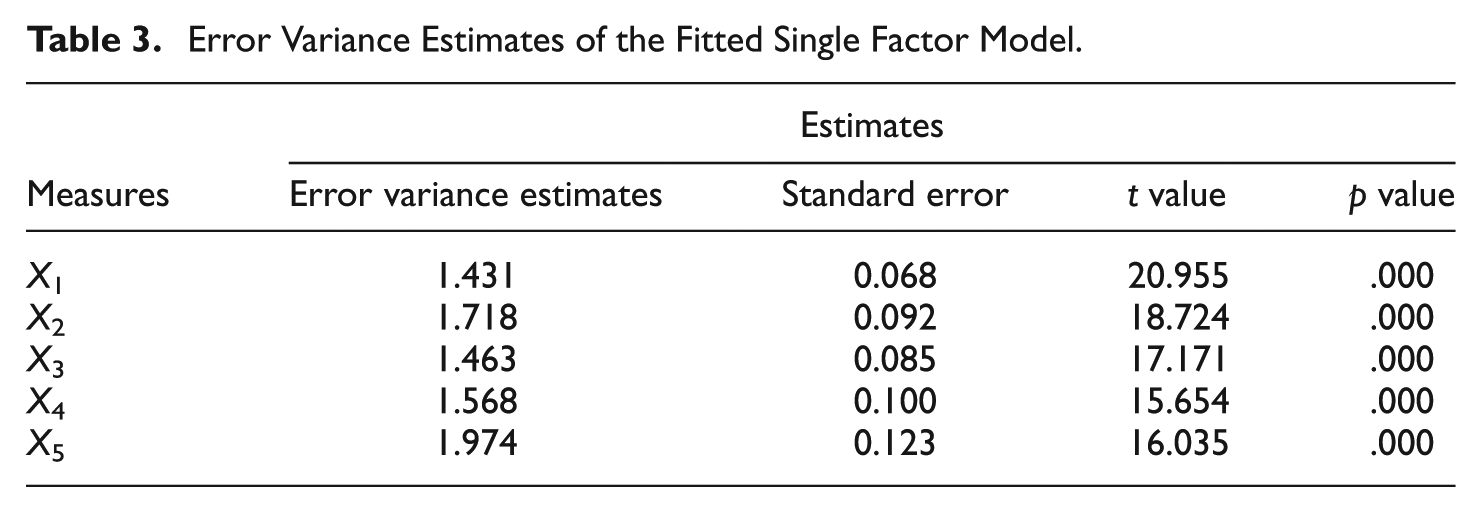
Employing the results in Table 3, we can now estimate the error variance in the first PC, which can be also conducted with the Mplus command file provided in the appendix. This leads to the following first PC error variance estimate (standard error in parentheses):

V \hat{a} r (E_{Y_{1}}) = 1.699 (. 047),

which is rather close to its population value calculated (determined) earlier in this section.

Utilizing next the bootstrap method (e.g., Efron & Tibshiriani, 1993), a 95% confidence interval is obtained for this error variance as

(1.613, 1.798),

which obviously covers that population value and has a left limit that is markedly above 0 (see the Mplus command file in the appendix for the needed source code, as well as the error variances in the model used for data generation).

Conclusion

Principal component analysis has served rather well the behavioral, biological, business, educational, engineering, medical, social, and natural sciences for the past more than 80 years since the landmark paper by Hotelling (1933). A particularly attractive feature of PCA is the (observed) variance maximization property, which allows for substantial reduction of complexity in many empirical data sets in these and related disciplines. While this is undoubtedly a very important and beneficial feature of PCA, whenever used for these aims, this article points out that it would be inappropriate to extend these optimality considerations to particular psychometric characteristics of individual principal components (PCs) and especially to the first PC. Specifically, the optimality feature of PCA pertains to observed variance, not error variance, and cannot be extended to imply or interpret PCA as (a) dealing away with error variance, or (b) producing perfectly reliable principal components, or (c) yielding principal components with reliability and criterion validity higher than the maximal reliability and criterion validity, respectively, which are possible to achieve with linear combinations of a given set of (homogeneous) fallible observed measures (with uncorrelated errors and for criteria uncorrelated with them).

The discussion in this note should not be seen as attempting to cast any shadow on the optimality properties of PCA, as these have long been rigorously demonstrated and well-known (e.g., Joliffe, 2002). Instead, the article merely aimed to examine properties of the PCs that are often of particular relevance in empirical educational and psychological research, especially when scholars are concerned with measurement related problems. In such settings, scientists are frequently confronted with observed measures that are not error-free but contain sizeable error of measurement that cannot be considered negligible. In those and related circumstances, of special importance can be the psychometric features of the PCs, in particular their error-proneness as well as bounded reliability and validity (criterion validity, for the setting used) as shown in this note.

We stress that this note assumed at least one error variance being positive, with all errors being uncorrelated, and hence the article did not intend to shed light on the psychometric features of principal components extracted from sets of observed fallible measures with at least two correlated errors. Similarly, the maximal reliability and validity related conclusions drawn in the article need not extend to cases where observed measures are not unidimensional (with uncorrelated errors) or used criteria variables are not uncorrelated with the error scores in those measures.

We finalize this article by pointing out that the psychometric properties of the principal components discussed here are not in any way inconsistent with their well-known optimality features, since the latter are such only with regard to observed variance. When part of it is error variance, however, rather than all of it being error-free variance, the findings presented in this note will be applicable, thus showing that any PC is error prone. Specifically, for a given set of measures where at least one is fallible (and their error terms are uncorrelated), any PC contains error and its error variance is bounded from above by the maximal error variance in the set. In addition, no PC can have then higher reliability or criterion validity than the maximally possible ones for a linear combination of the analyzed observed measures, when the latter adhere to a unidimensional model with uncorrelated errors (that are uncorrelated with the considered criterion as well). In conclusion, this note contributes to dispelling some myths about “perfect” reliability and extraction of “perfectly reliable” variance (or information) by PCs, which can be still found among or implied from some writings in the extant literature.

Footnotes

Appendix

Acknowledgements

We thank T. D. Little for a discussion on principal components and some of their psychometric features.

Declaration of Conflicting Interests

The author(s) declared no potential conflicts of interest with respect to the research, authorship, and/or publication of this article.

Funding

The author(s) received no financial support for the research, authorship, and/or publication of this article.

Notes

References

Bartholomew

D. J.

(1996). The statistical approach to social measurement. New York, NY: Academic Press.

Efron

Tibshiriani

(1993). An introduction to the bootstrap. Boca Raton, FL: Chapman & Hall.

Enders

C. K.

(2010). Applied missing data analysis. New York, NY: Guilford Press.

Härdle

Hlavka

(2007). Multivariate statistics. Heidelberg, Germany: Springer.

Hotelling

(1933). Analysis of a complex of statistical variables into principal components. Journal of Educational Psychology, 24, 417-441.

Howard

W. J.

(2012). Using principal component analysis to obtain auxiliary variables for missing data in large data sets (Doctoral dissertation). Retrieved from ProQuest Dissertations & Theses database. (UMI No. 3549761)

Howard

W. J.

Rhemtulla

Little

T. D.

(2015). Using principal components as auxiliary variables in missing data estimation. Multivariate Behavioral Research, 50, 285-299.

Johnson

R. A.

Wichern

D. W.

(2002). Applied multivariate statistical analysis. Upper Saddle River, NJ: Prentice Hall.

Joliffe

I. T.

(2002). Principal component analysis. New York, NY: Springer.

10.

Jöreskog

K. G.

(1971). Statistical analysis of sets of congeneric tests. Psychometrika, 36, 109-133.

11.

Muthén

L. K.

Muthén

B. O.

(1998-2015). Mplus user’s guide (7th ed.). Los Angeles, CA: Muthén & Muthén.

12.

Penev

Raykov

(2006). On the relationship between maximal reliability and maximal validity for linear composites. Multivariate Behavioral Research, 41, 105-126.

13.

Raykov

(2012). Scale development using structural equation modeling. In Hoyle

(Ed.), Handbook of structural equation modeling (pp. 472-492). New York, NY: Guilford Press.

14.

Raykov

Marcoulides

G. A.

(2006). A first course in structural equation modeling (2nd ed.). Mahwah, NJ: Lawrence Erlbaum and Associates.

15.

Raykov

Marcoulides

G. A.

(2008). An introduction to applied multivariate analysis. New York, NY: Taylor & Francis.

16.

Raykov

Marcoulides

G. A.

(2011). Introduction to psychometric theory. New York, NY: Taylor & Francis.

17.

Raykov

Marcoulides

G. A.

(2012). Basic statistics: An introduction with R. New York, NY: Rowman & Littlefield.

18.

Raykov

Marcoulides

G. A.

(2014). Population proportion explained variance in principal component analysis: A note on its evaluation via a large-sample approach. Structural Equation Modeling, 21, 588-595.

19.

Raykov

Marcoulides

G. A.

(2016). Evaluation of measurement instrument criterion validity in finite mixture settings. Educational and Psychological Measurement. Advance online publication. doi:https://doi.org/10.1177/0013164415613542

20.

SPSS, Inc. (2015). SPSS 22.0 Command Syntax Reference [Computer software]. Chicago, IL: Author.

21.

Timm

N. H.

(2002). Applied multivariate analysis. New York, NY: Springer.