Comparing Between- and Within-Group Variances in a Two-Level Study

Abstract

This note is concerned with examining the relationship between within-group and between-group variances in two-level nested designs. A latent variable modeling approach is outlined that permits point and interval estimation of their ratio and allows their comparison in a multilevel study. The procedure can also be used to test various hypotheses about the discrepancy between these two variances and assist with their relationship interpretability in empirical investigations. The method can also be utilized as an addendum to point and interval estimation of the popular intraclass correlation coefficient in hierarchical designs. The discussed approach is illustrated with a numerical example.

Keywords

between-group variance confidence interval hierarchical design latent variable modeling multilevel study variance ratio within-group variance

Multilevel studies have become very popular in the educational and psychological sciences over the past two decades (e.g., Goldstein, 2011). A main reason for this pronounced trend is the widespread realization that data collected in behavioral and social research are far more often of a hierarchical nature than previously assumed. In such investigations, however, the traditional assumption of independence of the units of analysis—an essential premise of conventional single-level statistical methods—cannot be considered fulfilled in general, because the characteristic feature of such studies is that subjects are clustered or nested within higher order units. As a result, these studied persons may not provide independent scores on response variables of interest. If the independence assumption is violated to a considerable degree then, standard methods based on it may yield seriously misleading results (e.g., Rabe-Hesketh & Skrondal, 2012; Raudenbush & Bryk, 2002).

In two-level models, which represent the majority of models currently used in the educational and behavioral disciplines with hierarchical data, the degree of this lack of independence of subjects’ outcome scores can be evaluated with the popular intraclass correlation coefficient (ICC). The ICC can be readily point and interval estimated, for instance, using a latent variable modeling approach (e.g., Raykov, 2011; see also, e.g., Raykov & Marcoulides, 2015, for the discrete response case), and three-level counterparts of the ICC can be similarly evaluated with suitable modifications of that approach (e.g., Raykov, 2010; Raykov, Patelis, Marcoulides, & Lee, 2016). While the ICC provides rather important information about the relationship of between-cluster to total variance in a two-level study, its empirical value is in general not easily interpretable by a practitioner. In particular, being a proportion between 0 and 1, or alternatively expressed as a percentage of total variance due to between group differences, the ICC is not always easy to interpret in substantive terms, especially when specific questions about the relationship of between-cluster to within-cluster variance rather than total variance are also of concern or even of more interest and importance to answer.

The present note provides a widely applicable method for enhancing the practical interpretability of the well-known variance decomposition strategy in hierarchical data sets. A latent variable modeling (LVM; e.g., B. O. Muthén, 2002) procedure is first outlined that permits routine point and interval estimation of the ratio of between- to within-group variance and complements the ICC evaluation in two-level settings. With this method, an empirical scientist can assess in arguably more pragmatically oriented terms the extent to which between-cluster variance is larger, or conversely is smaller, than within-cluster variance. In this way, he or she can utilize an alternative to relating the between-cluster variance to its sum with the within-cluster variance in the ICC, which could therefore be seen as confounding the two variances in its denominator. When one is interested in the extent to which between variance outperforms within variance, or vice versa, a researcher can thus evaluate directly their relationship and interpret straightforwardly in terms of relative size these two essential variances in a two-level study. We illustrate subsequently the proposed procedure with a numerical example, and conclude with a discussion of its limitations in empirical research.

Background, Notation, and Assumptions

In the remainder of this article, we denote by Y_ij the score on a response variable under consideration for the ith subject (level-1 unit) in the jth group (level-2 unit; i = 1, . . ., n_j, j = 1, . . ., J; cf., e.g., Raudenbush & Bryk, 2002). In educational and behavioral research, level-1 units are frequently students, patients, employees or repeated measurements, which are nested (clustered) within level-2 units such as schools, treatment centers, companies, departments, or persons longitudinally followed across several measurement occasions. We assume in the sequel that Y_ij is an (approximately) continuous outcome measure (see also Conclusion section).

At the outset of a multilevel modeling process, the (fully) unconditional two-level model is defined by the next two equations that represent its within-group and between-group parts (models), respectively:

Y_{ij} = β_{0 j} + r_{ij},

and

β_{0 j} = γ_{00} + u_{0 j} .

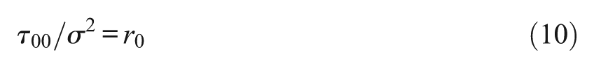
In this unconditional model, r_ij is the deviation of Y_ij from the mean β_0j of the jth group, with this difference assumed to be normally distributed with mean 0 and variance σ² (i = 1, . . ., n_j, j = 1, . . ., J). The variance σ² is typically referred to as within-group (within-cluster) variance and is assumed to be positive in this article. In the second equation of the model, u_0j is the jth group’s mean deviation from the grand mean γ₀₀, which discrepancy is also assumed normal, with zero mean and variance τ₀₀ (j = 1, . . ., J). The variance τ₀₀ is usually referred to as between-group (between-cluster) variance.

By substitution, the associated combined or mixed model is

Y_{ij} = γ_{00} + u_{0 j} + r_{ij}

(i = 1, . . ., n_j, j = 1, . . ., J). Equation (3) presents the basic decomposition used to obtain the popular ICC, which is defined as the ratio of between-group variance to its sum with within-group variance:

ρ = τ_{00} / (τ_{00} + σ^{2}) .

As seen by its definition, the ICC represents the proportion (percentage after multiplying by 100) of observed variance that is due to between-cluster differences, and contains rather useful information in many empirical circumstances. Given that the sum or between and within group variance features in the denominator of the ICC, one may argue that (the denominator of) the ICC “confounds” between- and within-cluster differences. This property of the ICC may thus be seen by a practitioner as somewhat distracting, who may actually be more interested in the extent to which between-group differences say surpass or are larger than within-group differences, or vice versa. For example, an educational policy analyst may be concerned with evaluating the extent to which school differences may be overwhelming student differences within each school, or alternatively may be interested in evaluating the degree to which within-cluster differences surpass between-cluster variability, with important policy related implications in either situation. In that case, the ratio of these two variances, defined as

r = τ_{00} / σ^{2},

can be seen as being of additional or possibly even greater relevance to him or her than the ICC.

While the between-to-within variance ratio r can be obtained from the ICC via corresponding algebraic rearrangements, the availability of a procedure to automate the calculation and provide point and interval estimation of this ratio would be quite helpful to empirical researchers. In addition, there do not seem to be widely available rules-of-thumb that could be used to evaluate in substantive terms an arbitrary ICC estimate in a given study; with this in mind, one might argue that a sample ICC estimate is in general not readily interpretable. By way of contrast, an estimate of the ratio (Equation 5) directly represents the number of times between-group variance is larger, or conversely smaller, than within-group variance. With this feature, the quantity r may be viewed by some applied researchers of additional if not greater value in certain circumstances than the ICC. We describe next a widely applicable procedure that readily accomplishes point and interval estimation of the ratio r in Equation (5).

A Latent Variable Modeling Procedure for Evaluation of the Ratio of Between-Group to Within-Group Variance in Two-Level Models

Point and Interval Estimation

Revisiting the unconditional model in Equations (1) and (2), or its mixed model version in Equation (3), we notice that it involves two latent variables (cf. Raykov, 2011). Indeed, none of the variables u_0j or r_ij appearing in the right-hand side of Equation (3) is measured or observed, unlike the recorded scores Y_ij (i = 1, . . ., n_j, j = 1, . . ., J). In addition, each corresponding level-2 or level-1 unit is associated with an individual realization of the random variable u_0j or r_ij (i = 1, . . ., n_j, j = 1, . . ., J). Hence, one can view Equations (1) and (2) as defining a latent variable model. This model can be readily fitted to a given empirical data set using popular LVM software, such as Mplus (L. K. Muthén & Muthén, 2015).

This LVM application will yield estimates of the between and within group variances as well as associated standard errors and covariances, and hence a point estimate of the ratio (Equation 5) of interest in this article. Subsequently using the delta method (e.g., Raykov & Marcoulides, 2004), a confidence interval (CI) for this ratio r, for any prespecified confidence level can be obtained. More specifically, because Equation (5) involves two variances, r can never be negative, that is, the variance ratio r is a population parameter that is bounded from below (i.e., 0 is its lower bound).¹

Therefore, to obtain a CI for r at a given confidence level, say (1 − α)100% (0 < α < 1), we can utilize a monotone transformation approach (e.g., Browne, 1982). Accordingly, one needs to take first the (natural) logarithm of the estimator of r, log(r), and then using its standard error (obtained with the delta method) furnish a symmetric (1 −α)100% CI by subtracting and adding z_α/2 times that standard error to log(r), with z_α/2 being the (1 −α/2)th standard normal quantile. Finally, via exponentiation of the last CI’s limits, we obtain the same confidence level CI limits of the critical ratio r of initial interest. (Further discussion and details on this approach to CI construction are provided in Raykov & Marcoulides, 2014, in an analysis of incomplete data context, and we refer to that source.) All these activities leading to a CI for the variance ratio r, are implemented in the R-function “ci.r” provided in the appendixes to this note along with the Mplus source code needed to fit the two-level model (1) and (2) (cf. Raykov, 2011).

We illustrate in a subsequent section this point and interval estimation procedure using an empirical example.

Testing Simple and Composite Hypotheses About the Ratio of Between to Within Variance

While the ratio (Equation 5) is nonnegative and in practical terms could be seen as always positive (see Note 1), it may be of relevance in some settings to test the null hypothesis of it being 0, that is,

H_{0} : r = 0

In those cases, we mention in passing that the test of this hypothesis is in fact implemented in popular software, for instance Mplus, since null hypothesis (6) is equivalent to the hypothesis of vanishing between-group variance, that is, $H_{0}^{*} : τ_{00} = 0$ . The two-tailed p-value for the latter hypothesis is routinely provided by the software used, and dividing it by 2 renders the sought p-value for the null hypothesis (6), owing to the fact that formally the alternative hypothesis, $H_{1}^{*} : τ_{00} > 0$ , is one-tailed (e.g., Rabe-Hesketh & Skrondal, 2012).²

Further, for any given number r₀ > 0, which is of substantive interest to a researcher, a test of the hypothesis

H_{0} : r = r_{0}

at a prefixed significance level α against the bidirectional alternative of r not being equal to r₀, is directly carried out by checking if r₀ is contained in the corresponding CI obtained as above, with no rejection of hypothesis (7) in that case and rejection otherwise (e.g., Raykov & Marcoulides, 2008).

If the hypothesis

H_{0} : r \geq r_{0}

is to be tested against the alternative

H_{0} : r < r_{0},

at the significance level α, one can proceed in a similar way. Specifically, if the corresponding CI is entirely above r₀, then H₀ can be considered not rejected; if that CI is entirely below r₀, H₀ can be rejected. If the CI covers r₀, however, one may (a) conclude that the analyzed data set does not provide sufficient evidence to make a decision of rejection or no rejection of the tested null hypothesis and (b) recommend a replication study with a larger sample, in the hope that due to higher power then the CI will be sufficiently narrow to enable a decision as indicated above in this paragraph. When the null and alternative hypotheses have respectively the reverse directions to those in hypotheses (8) and (9), one proceeds conversely by complete analogy, using the same confidence level CI.

Last but not least, if the simple hypothesis (7) is to be tested against a one-tailed alternative, i.e., r > r₀ or r < r₀, which is of substantive relevance, then one can proceed as follows. First, impose in the fitted model (1) and (2) the nonlinear constraint

τ_{00} / σ^{2} = r_{0}

and halve the resulting p-value associated with the pertinent likelihood ratio test (chi-square goodness of fit value) in this nested model (cf. Rabe-Hesketh & Skrondal, 2012). If the sample estimate of r is in the direction of the alternative and this halved p-value is lower than a preset significance level, for example, α, rejection of the H₀ in (7) is warranted; otherwise that null hypothesis H₀ is not rejected.

We demonstrate next on empirical data the preceding discussion in this note.

Illustration on Data

We employ for our aims in this section data from a study conducted by Mortimore, Sammons, Stoll, Lewis, and Ecob (1988; see du Toit & du Toit, 2001, also for the original data). To this end, we use scores on a Mathematics test that stem from N = 1192 students attending G = 49 schools randomly sampled from the London area. We begin by fitting the unconditional latent variable model (1) and (2) (cf. Raykov, 2011), whose fit is perfect since it is saturated: chi-square value (χ²) = 0, degrees of freedom (df) = 0. (The needed Mplus source code is provided in Appendix A, with annotating comments following an exclamation mark within pertinent row.) The obtained estimates thereby of the within-group and between-group variances as well as their ratio r are correspondingly as follows (standard errors are presented in parentheses, and hat denotes estimate):

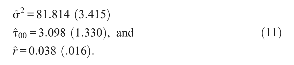
\begin{matrix} {\hat{σ}}^{2} = 81.814 (3.415) \\ {\hat{τ}}_{00} = 3.098 (1.330), and \\ \hat{r} = 0.038 (. 016) . \end{matrix}

Using next the R-function “ci.r” in Appendix B with these results for the variance ratio, r, its 95% CI is furnished as (.017, .087). This CI could be interpreted as a range of plausible values, at the 95% confidence level, for the number of times the between-school variance on this test is smaller than the within-school variance on it, with this range stretching from 2% to 9% (rounded off). That is, one could consider plausible (at this confidence level) that the between-school variance on the used test is approximately between 11 and 50 times smaller than the within-school variance. This result may be interpreted as suggesting that the between-school differences on the mathematics test under consideration represent a small fraction of the within-school differences in the student scores on it, and that schools are rather homogeneous on this test relative to student differences within school. Further substantive interpretation of this funding (confidence interval) would be left to the expert in the pertinent subject-matter field.

Conclusion

This article was concerned with a procedure for examining the degree to which between-cluster differences surpass or alternatively are dominated by within-cluster differences in two-level studies. A latent variable modeling method for point and interval estimation of the ratio of between to within group variance on a response variable was outlined. The discussed approach is useful in multilevel studies as a complement to the popular ICC and contributes to a more pragmatically oriented interpretation of the relationship between within- and between-cluster variances. As a possible addendum to point and interval estimates of the ICC (e.g., Raykov, 2011), the present procedure permits empirical researchers to reach also more informed conclusions about the extent to which the classical assumption of independence of units of analysis may be violated (see also Rabe-Hesketh & Skrondal, 2012).

The described method possesses several limitations that need to be pointed out. While it can be readily extended to three-level studies, for example, following the developments in Raykov et al. (2016), the procedure is presently available for (approximately) continuous normal response variables (see Raykov & Marcoulides, 2015, for a possible extension approach to the discrete case). While it could be argued that up to mild violations of normality could be handled via robust maximum likelihood (ML) estimation unless with piling of cases at a scale end (e.g., L. K. Muthén & Muthén, 2015), which may be potentially also applicable with items having at least five to seven response options, additional research is needed to address this conjectured robustness. Furthermore, the underlying estimation procedure is best used with large samples both with respect to the number of clusters and observations within them (e.g., Raudenbush & Bryk, 2002; Raudenbush & Xiao-Feng, 2001). This stems from the fact that the method rests on ML estimation that itself is grounded in an asymptotic statistical theory. Future research is thus also encouraged that should be concerned with the development of possible guidelines that could be followed in evaluating sample size requirements of level-2 and level-1 units, at which one could rely in practice on the ML asymptotic theory.

In conclusion, this article provides educational and behavioral researchers with a readily applicable means of interval estimation for the ratio of between-group to within-group variance, which allows more pragmatically oriented interpretation of the fundamental variance decomposition in hierarchical designs and aids more informed decisions about the degree of interdependence of outcome scores on studied response variables. The outlined procedure may also be particularly beneficial as a complement to the popular ICC, in that it permits examining more thoroughly the clustering effect in multilevel data and could help in choosing if needed between traditional, single-level models and more complex, multilevel models for use in ensuing analyses.

Footnotes

Appendix A

Appendix B

Acknowledgements

We thank G. Mels for a valuable discussion on bounded parameter estimation.

Declaration of Conflicting Interests

The author(s) declared no potential conflicts of interest with respect to the research, authorship, and/or publication of this article.

Funding

The author(s) received no financial support for the research, authorship, and/or publication of this article.

Notes

References

Apostol

T. G.

(2013). Calculus. New York, NY: Wiley.

Browne

M. W.

(1982). Covariance structures. In Hawkins

D. M.

(Ed.), Topics in applied multivariate analysis (pp. 72-141). Cambridge, England: Cambridge University Press.

du Toit

S. H. C.

du Toit

(2001). Interactive LISREL 8: User’s guide. Lincolnwood, IL: Scientific Software International.

Goldstein

(2011). Multilevel statistical models. London, UK: Arnold.

Mortimore

Sammons

Stoll

Lewis

Ecob

(1988). School matters, the junior years. Wells, England: Open Books.

Muthén

B. O.

(2002). Beyond SEM: General latent variable modeling. Behaviormetrika, 29, 87-117.

Muthén

L. K.

Muthén

B. O.

(2015). Mplus user’s guide. Los Angeles, CA: Muthén & Muthén.

Rabe-Hesketh

Skrondal

(2012). Multilevel and longitudinal modeling with Stata. College Station, TX: Stata Press.

Raudenbush

S. W.

Bryk

A. S.

(2002). Hierarchical linear models. Applications and data analysis methods (2nd ed.). Thousand Oaks, CA: Sage.

10.

Raudenbush

S. W.

Xiao-Feng

(2001). Effects of study duration, frequency of observation, and sample size on power in studies of group differences in polynomial change. Psychological Methods, 6, 387-401.

11.

Raykov

(2010). Proportion of third-level variance in multilevel studies: A note on an interval estimation procedure. British Journal of Mathematical and Statistical Psychology, 63, 417-426.

12.

Raykov

(2011). Intra-class correlation coefficients in hierarchical designs: Evaluation using latent variable modeling. Structural Equation Modeling, 18, 73-90.

13.

Raykov

Marcoulides

G. A.

(2004). Using the delta method for approximate interval estimation of parametric functions in covariance structure models. Structural Equation Modeling, 11, 659-675.

14.

Raykov

Marcoulides

G. A.

(2008). An introduction to applied multivariate analysis. New York, NY: Taylor & Francis.

15.

Raykov

Marcoulides

G. A.

(2014). Identifying useful auxiliary variables for incomplete data analyses: A note on a group difference examination approach. Educational and Psychological Measurement, 74, 537-550.

16.

Raykov

Marcoulides

G. A.

(2015). Intraclass correlation coefficients in hierarchical design studies with discrete response variables: A note on a direct interval estimation procedure. Educational and Psychological Measurement, 75, 1063-1070.

17.

Raykov

Patelis

Marcoulides

G. A.

Lee

C.-L.

(2016). Examining intermediate omitted levels in hierarchical designs via latent variable modeling. Structural Equation Modeling, 23, 111-115. doi:10.1080/10705511.2014.938186