Bayesian and classical statistical approaches are based on different types of logical principles. In order to avoid mistaken inferences and misguided interpretations, the practitioner must respect the inference rules embedded into each statistical method. Ignoring these principles leads to the paradoxical conclusions that the hypothesis could be less supported by the data than a more restrictive hypothesis such as , where and are two population means. This article intends to discuss and explicit some important assumptions inherent to classical statistical models and null statistical hypotheses. Furthermore, the definition of the p-value and its limitations are analyzed. An alternative measure of evidence, the s-value, is discussed. This article presents the steps to compute s-values and, in order to illustrate the methods, some standard examples are analyzed and compared with p-values. The examples denunciate that p-values, as opposed to s-values, fail to hold some logical relations.
In social sciences, the majority of the events are contingent, full of uncertainties and permeated by nuisance variables. For instance, cognitive skills are affected by a number of factors such as education, culture, age, tiredness, genetics, and so on. It is impractical to contemplate all factors that influence a specific cognitive skill. Probability and statistical models are mathematical tools used to handle contingent and uncertain events (Fisher, 1955; Kadane, 2011; McCullagh, 2002). These tools are defined in terms of sets and functions, which are fully consistent with the modern formulation of mathematics.1
Statistical models are employed to make inferences about unknown quantities and to test the consistency of scientific statements with the observed data (Fisher, 1955). However, statistical models have domains of applicability, internal rules, principles, limitations, and so on (Fisher, 1922; Dempster, 1968; Hájek, 2008). It is important to understand those internal features in order to avoid inadequate interpretations obtained from prohibited inferential rules (Berger & Sellke, 1987; Fisher, 1955; Kempthorne, 1976; Lavine & Schervish, 1999).
The main goal of this article is to discuss some hidden assumptions underlying the classical statistical models2 and null hypotheses, see sections “Statistical Models” and “Scientific and Statistical Hypotheses.” The section “Definition of p-Values” discusses the formal definition of a p-value. The section “Problems of p-Values and an Alternative Measure of Evidence” presents its limitations and reviews a new classical measure of evidence, called s-value, that overcomes some limitations of the p-value. The penultimate section “Numerical Examples” provides some standard examples on testing population averages that illustrate the following feature of p-values: They do not respect the reasoning of the logical consequence. The reasoning of logical consequence is as follows: If one hypothesis implies another one , then, by the logical consequence, we would expect more evidence against than that against . For example, let and be two population means. From p-values, it is possible to obtain the following striking result: with the same observed data, one can find more evidence against than against , even though the latter necessarily implies the former. The final section concludes the article recapitulating the main points discussed in the article.
Statistical Models
It is difficult to introduce probability and statistical models by adopting an easy language without ambiguity. This article avoids the set-theoretic notation and will not introduce the primary probability space where all quantities are well defined (e.g., random variables, statistics, estimators, induced spaces, etc.). The reader should be aware that the language used here is informal, and to avoid ambiguities it will be required to make many textual caveats. The reader is referred to Cox and Hinkley (1974), Schervish (1995), Lehmann and Casella (1998), and McCullagh (2002) for a detailed discussion on statistical models.
Roughly speaking, the steps before choosing a statistical model are (not necessarily in this particular order) the following:
Define the objectives of the study
Define the population of interest
Define the quantities of interest
Define an adequate experiment to collect the sample
The practitioner must have prior knowledge to construct an appropriate experiment to access the quantities of interest, for each field has its idiosyncrasies that must be taken into account. The experiment may be randomized in specific strata or layers or clusters (different treatments, genders, groups of risk, and so on), and these considerations should guide the researcher to choose the class of probability distributions that will be considered in the statistical model. Typically, in scientific experiments, there are direct observable quantities (age, gender, measured height and weight, etc.) and unobservable quantities (intelligence, “feelings of morale,”“sense of belonging,” etc.). These quantities might be either random or nonrandom and are ingredients of a statistical model. All random quantities must be well-defined in a probability space.
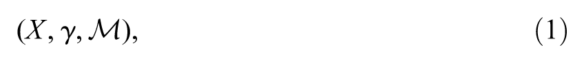
In this article, random observable quantities are denoted by uppercase Latin letters, say or , and their observed counterparts are denoted by lowercase Latin letters, say or . Random and nonrandom unobservable quantities are denoted by the Greek letters and , respectively. The unobservable random quantities are called latent random variables (Bollen, 2002). Let us informally represent a statistical model by the triplet
where represents the observable random variables, represents the latent random variables and is a family containing joint probability (density) functions of the random variables, that is, , where is a possible joint probability (density) function of , for each . It should be clear that is an indexer of possible probability distributions, it is not a random variable. Through residual analyses, one can verify empirically if the family is adequate or inadequate to model the observable data. It is not possible to assure that the family contains the generator mechanism of the data, that is, the mechanism that effectively generates the data. Furthermore, the data’s generator mechanism might not even be translatable in terms of probability distributions.
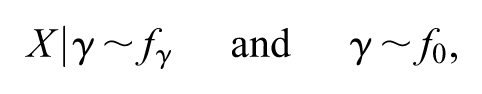
When the probability distribution that governs the random quantities is known, then contains only one element, namely , where is the joint probability (density) function of the observable and unobservable random variables, with
where is the probability (density) function of the random variable given and is the probability (density) function of the random variable . Recall that in this latter case, it is assumed that the joint probability distribution that governs the random quantities is known. In this context, it is possible to provide full probabilistic descriptions of the random quantities (mean, variance, quantiles, marginal probabilities, joint probabilities, conditional probabilities, etc.). As aforementioned, in practice it is difficult (or even impossible) to known the generator of the random quantities and the family typically has more than one element.
The formal statistical model is defined with sigma-fields and a family of probability measures (see, for instance, Lehmann & Casella, 1998; Lehmann & Romano, 2005; McCullagh, 2002; Patriota, 2013). The reader must keep in mind that Model (1) is a simplified version that shall help us understand some important features of the classical statistical model and the null hypothesis statistical testing.
Scientific and Statistical Hypotheses
In science, it is common to formulate statistical hypotheses to test scientific statements. A nontrivial step is to translate a scientific statement into statistical language. In the classical paradigm, a statistical hypothesis is a statement about probability distributions that potentially govern the experimental data. That is, in order to create a statistical hypothesis, one must be able to transform a scientific statement in terms of probability distributions. For instance, the statement “this coin is not biased” is typically transformed into “,” that is, the following is taken as a hidden principle:
“This coin is not biased” AND “”
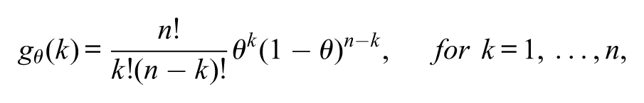
The theoretical assumptions are made from the specific features of the chosen experiment. One experiment may be performed by independently throwing times the coin over a smooth surface. The observable random variable is the number of times the coin turned up heads. In this simplified version, no latent variables are considered. Assuming that the coin cannot land on its edge, one statistical model that can represent this experiment is the binomial model , where with
where is the usual factorial notation, is the probability that the studied coin turns up head and is the probability that the coin turns up heads exactly times in the performed experiment. The scientific statement and its statistical counterpart are related by
“This coin is not biased” AND “”
The null hypothesis is then represented by , that is is a statement about probabilities: “if the coin is not biased, then [by the above principle and model assumptions] the probability that the coin turns up head is 0.5.” Notice that, unless the practitioner is totally certain of the theoretical assumptions, evidence to reject does not mean evidence to reject the scientific statement. Indeed, we have that implies that either “This coin is biased” or “at least one of the theoretical assumptions is not adequate.”
Under the null hypothesis , the statistical model reduces to , where . In general, the alternative hypothesis is defined to be and under this alternative hypothesis the statistical model is , where . Notice that the union of both restricted families under and must be the original family, that is, . This means that the original statistical model can be partitioned into two separated statistical models, namely the one generated under and the other generated under .
In the binomial model, it is implicitly assumed in the “Theoretical assumptions” that “ (this coin turns up head)” does not change over all throws. Of course, this assumption is oversimplified for actual processes, since in each throwing the coin is submitted to impacts causing microscopic cracks, warps and, consequently, modifications in “ (this coin turns up head)” over time. Other statistical models can be implemented by relaxing some of the imposed suppositions: (1) latent random variables can be incorporated to model dependence among the coin flips and (2) covariates may be inserted to model variations in . That is, by changing some “Theoretical assumptions,” many statistical models could be used to model the outcomes of the very same experiment.
The concept of coin bias can be further elaborated. One may prefer to relate the statement “this coin is not biased” with the structural topology of the coin, for example, types of symmetries around the mass center of the coin, and so on. Under this latter definition, it is possible to define degrees of bias based on a measure of symmetry and another completely different statistical model will emerge. This simple example illustrates the complexity of statistical models and the problem of translating a simple scientific hypothesis into a statistical language. This example is applied in problems with binary outcomes; for instance, the random variable may be defined to be the number of allergic patients, out of , who react positively to a specific treatment.
Logical Relations Between the Null and Alternative Statistical Hypotheses
In general, a full statistical model is initially specified . After establishing the null and alternative hypotheses and , reduced statistical models emerge and under these hypotheses, respectively, where . The null hypothesis states “at least one marginal probability distribution listed in generates the observable random variable”. Notice that, the alternative hypothesis is not the negation of . Moreover, the negation of the null hypothesis cannot be written in statistical terms, since includes all possible mechanisms, not necessarily probabilistic ones, that could generate the observable variables . The negation of is
“It is not the case that ‘at least one marginal probability distribution listed in generates the observable random variable ’.”
Therefore, does imply , but does not imply . Therefore, the practitioner should be aware that a decision between and is very limited, since there is an option beyond the disjunction “.” As does not imply , “” is a valid third option. These logical relations lie at the core of many controversies about null hypothesis statistical testing. For instance, Bayesian procedures typically use a prior probability such that . The problem with this latter procedure is that it gives the impression that the alternative hypothesis is the negation of the null hypothesis, since by the probability properties the following is a consequence: , which implies probability zero to the logically valid third option ; which means, in some sense, that the practitioner is sure that this third option is not relevant for the statistical analysis. This is exactly what is considered in the analysis derived by Trafimow (2003), which will be discussed in this section.
The statistical hypotheses and are not necessarily exhaustive, because, as said previously, the family might not contain the data’s generator mechanism. Even after making post-data analyses to verify whether the model assumptions are adequate (through residual analyses, simulated envelopes and so on; see Atkinson, 1985; Cook, 1977, 1986, for more details), one cannot guarantee that “” is not a relevant option. For the sake of analysis, let us assume that and are exhaustive and mutually exclusive hypotheses, then the following inference rules are valid:
Empirical evidence to reject is empirical evidence to accept : .
Empirical evidence to reject is empirical evidence to accept : .
However, if the disjunction “” is not exhaustive, then the preceding inference rules are not valid anymore, rather we have the following
Empirical evidence to reject is not necessarily empirical evidence to accept : .
Empirical evidence to reject is not necessarily empirical evidence to accept : .
Recall that, as discussed previously, to accept (or reject) is not the same as to accept (or reject) the scientific hypothesis, unless the practitioner is certain of the theoretical assumptions, which is scarcely the case. The above analysis explicits the main difference between uncertain inference and decision theory as professor Sir Ronald Fisher argued in some of his articles (Fisher, 1935, 1955). On one hand, if the disjunction “” is not exhaustive, we have uncertain inference and more difficulties arise, for the universe of possibilities is not closed (we have to deal with the third option). Under this context, the practitioner must not use the inferential rules “” and “.” On the other hand, if the disjunction “” is (assumed to be) exhaustive, we have decision theory and the space of decisions becomes well defined, for the inferential rules “” and “” are valid. It is important to note that the classical statistical model is sufficiently general to allow these two situations discussed above:
The Fisherian procedure considers that “” is not necessarily exhaustive. P-values were initially defined to be used in this situation, they were designed to detect discrepancies between the null hypothesis and the observed data. It is not required to define an alternative hypothesis; in this context, as aforementioned, some inference rules should not be employed. A very small p-value indicates a large discordance between the postulated null hypothesis and the observed data, however, a non-significant p-value does not indicate evidence in favor of the null hypothesis. Fisher (1955) says, “The attempt to reinterpret the common tests of significance used in scientific research as though they constituted some kind of acceptance procedure and led to ‘decisions’ in Wald’s sense, originated in several misapprehensions and has led, apparently, to several more” (p. 69).
The Neyman–Personian procedure considers that “” is exhaustive. This is the case for the statistical tests developed by Neyman and Pearson. They developed the most powerful test for a fixed significance level (the probability of rejecting the null when it is false). A rejection region is built based on this procedure and a decision is taken by verifying whether the observed sample lies or not in the rejection region. The Bayesian procedure is more aligned with the Neyman–Personian procedure than with the Fisherian, for at least some logical principles are shared between them. Naturally, regarding “” as exhaustive is only an artificial assumption to resolve a statistical problem; the statistician may not consider this as True in an ontological sense.
The above two perspectives lead to different types of statistical inferences. Moreover one cannot be used to invalidate the other, since they use different principles (one considers that “ OR ” is exhaustive and the other does not) which lead to different rules of inferences. Many papers in the scientific literature confound these two intrinsically different perspectives (see Hubbard, Bayarri, Berk, & Carlton, 2003, and references therein).
Recently, Trafimow (2003), by explicitly assuming that “” is exhaustive, defined p-values by conditional probabilities and employed the rules of conditional probabilities to show that p-values are internally flawed. He wrote “the Bayesian analyses presented earlier not only suggest possible problems with null hypothesis significance testing procedure (NHSTP) but also demonstrate when these potential problems become actual problems and when they do not.”Trafimow (2003) deliberately applied the Bayesian reasoning to analyze the p-values’ behavior and to conclude that they are flawed. In a recent editorial note published in the Basic and Applied Social Psychology (BASP), Trafimow and Marks (2015) communicated that the NHSTP was banned from BASP. The editorial note said that
prior to publication, authors will have to remove all vestiges of the NHSTP (p-values, t-values, F-values, statements about significant differences or lack thereof, and so on). (Trafimow & Marks, 2015, p. 1, in Answer to Question 1)
The attempts of writing classical statistics with Bayesian notation is a strong source of misinterpretations and controversies. One reason, as discussed previously, is because their logical reasoning are different. Another reason is that some conditional statements in the classical statistics are not probabilistic statements. The p-value is formally defined in the next section; as the reader shall see, it has nothing to do with the formal definition of conditional probabilities and it is not connected directly with the Bayesian interpretation. In my view, the main problem with the subjective Bayesian approach is that it excludes all possible probability measures outside from the very beginning of the statistical analysis.3
Definition of p-Values
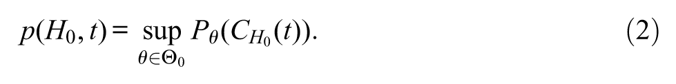
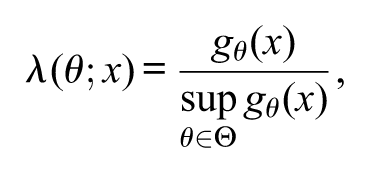
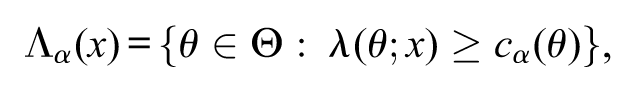
A p-value is built with the purpose of capturing a disagreement between the observed data and the postulated null hypothesis. In this context, a first step is to define a positive real statistic , it is a function of the random sample which depends on the null hypothesis , such that: the larger its observed value , the stronger is the disagreement between the observed data and the null hypothesis (Cox, 1977; Mayo & Cox, 2006; Patriota, 2013). The set describes all sample values that have stronger disagreements with the postulated null hypothesis than the observed one. This set has three important elements, namely, the null hypothesis of interest , the random statistic and the observed statistic . Note that strongly depends on .
If is small compared to the total set , then the observed experiment provides strong evidence against ; this happens when the observed is large enough to lie in the extreme right tail of the statistic ’s distribution. One way to measure the size of is through probabilities. As the null hypothesis states probability distributions that represent the scientific statement of interest, the p-value is computed for the case with the highest probability in . Let us consider the model without latent variables , where is the set of probability (density) functions restricted under the specifications of . Let be the probability measure associated with , that is, if is a probability function, then and if is a probability density function then , where is a measurable set. The p-value is formally defined by
Therefore, as is (greater than or equal to) the case with the highest probability in , the smaller the value of , the larger is the evidence against . Formula (2) explicitly says that the classical p-value is not a conditional measure in the probabilistic sense, it is instead a conditional measure in the possibilistic sense. The reader should notice that the usual representation p-value is inadequate, since (a) the probability is meaningless in the context of classical statistical models and (b) the conditional probability is being misused, since its formal definition is being ignored. The conditional probability is defined by , where and and are events of the same type (they must be listed in the same sigma-field). As for random variables, the conditional probability is defined analogously for the probability (density) function . In classical statistics, the events and are not of the same type, for they are not listed in the same sigma-field; otherwise it is a Bayesian-like analysis.4 In classical statistics, there is not a probability distribution defined over the subsets of and as cannot (even ideally) list all possible measures, a probability measure over the subsets of would be conceptually ill-defined.5
Technical Remark: For each observed statistic , the quantity is fixed while is random for each . If, for each fixed , for all , then the statistic will be (informally) said to be ancillary to , and then the “sup” operation in (2) vanishes. This happens in many problems under normal distributions when the interest is centered in testing population means and/or variances. In this context, if is a continuous random variable and it is ancillary to , the distribution of is uniform between 0 and 1. This allows the practitioner to interpret a p-value in terms of ideal replications of the performed experiment:
“if the performed experiment were repeated times, then it is estimated that of those experiments would produce p-values smaller than the observed one.”
This interpretation of repeating sampling from the same population is criticized by Fisher (1955). The main argument follows: “if we possess a unique sample in student’s sense on which significance tests are to be performed, there is always, . . ., a multiplicity of populations to each of which we can legitimately regard our sample as belonging” (see section 2 of Fisher, 1955, for more details).
Problems of p-Values and an Alternative Measure of Evidence
The p-value is a statistical tool to verify a possible discrepancy between a fixed null hypothesis and the observed data. Nevertheless, there is a serious limitation in the use of p-values in nested hypotheses. Consider that the p-value’s computation under is extremely complicated. Let be an auxiliary hypothesis such that , that is, if is true, then is true. By logical reasoning: if is false, then must also be false. The practitioner, led by this logical reasoning, would compute the p-value under and conclude that if there is evidence to reject , that is, the p-value computed under is significantly small, then there must be evidence to reject . However, p-values do not allow this latter logical reasoning. That is, it is not guaranteed that , see the next section for numerical examples. This happens because the test statistic is built for a specific null hypothesis, therefore, the respective p-value is valid only for this specific null hypothesis; for more details, see, for instance, Schervish (1996) and Patriota (2013). In previous work, Patriota (2013) proposed an alternative classical measure of evidence that meets the above logical reasoning; it is called s-value and will be presented in what follows.
The general purpose of the s-value is almost the same as of the p-value: to verify a discrepancy of null hypotheses with the observed data, but maintaining all logical consequence among null hypotheses. In order to define s-values, let us consider the simplest statistical model without latent variables , where and let be the probability measure associated with the probability (density) function . The likelihood-ratio statistic is
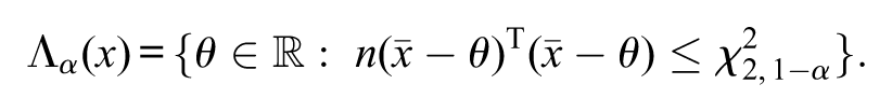
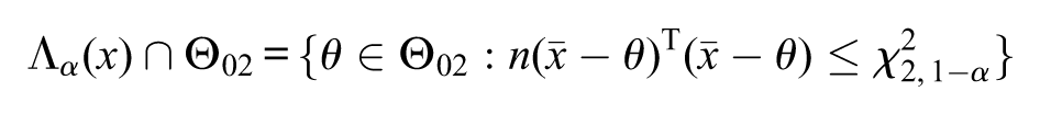
provided that . Notice that, for all . The likelihood-ratio confidence region with significance level is defined by
where
and . The following equivalent notation may be used
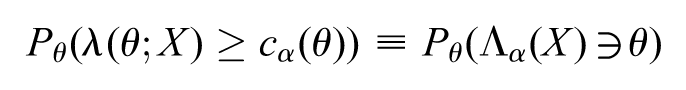
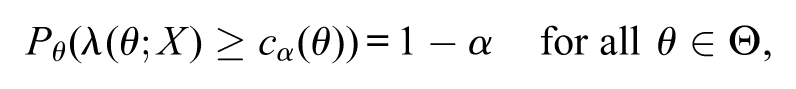
The quantity is the probability of to contain , under the measure . This is the formal definition of a general confidence region for the parameter (Schervish, 1995).
For some statistical models (normal distribution in general), the following occurs:
in this case, the confidence region is said to be exact. For exact confidence regions, the value is the quantile of the random variable . Observe that contains all ’s that generate likelihood values greater than (or equal to) times the largest likelihood value, namely, . This set is intuitive, for it contains the optimal values for according to the likelihood function. The definition of the s-value follows.
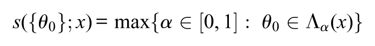
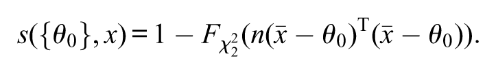
Definition 1. Let be a nonempty parameter subset related with and let be the likelihood-ratio confidence region with significance level . Then, the s-value is defined by
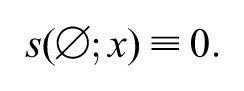
If , define
This definition is valid for general hypotheses. Let and be two parameter subsets related with the hypotheses and , respectively. In this context, if , then ; Patriota (2013) showed that the following always occurs . A possible interpretation for the s-value, under the regular conditions stated in Patriota (2013) and assuming that is nonempty and closed, reads
“ is equal to the maximum significance level such that and have at least one element in common.”
The smaller is, the more distant is from the maximum likelihood estimate of and, consequently, the more unlikely is according to the likelihood-ratio confidence region. Observe that, if , where is a given vector (or number if ), then and the s-value reduces to
and its interpretation reads
“ is equal to the maximum significance level such that contains .”
Therefore, the farther away is from the center of , which in regular conditions is the maximum likelihood estimative, the more the observed evidence is against . Patriota (2015) studied the likelihood-ratio statistic as a measure of evidence and compared it with the s-value and posterior distributions. González, Castro, Lachos, and Patriota (2016) employed the s-value to study confidence sets for observed samples.
Types of Decisions
In this section, some types of decisions are studied. Let be the maximum likelihood estimative of , then, under regular conditions (Cox & Hinkley, 1974, Chap. 9), we have that and it exists.
First Case
No alternative hypothesis is defined, then the general advice of this paper is to use the s-value as a thermometer of discrepancy between null hypotheses and the observed data. The smaller is , the stronger is the evidence against . Patriota (2013) showed that if , then and the observed data produce no evidence against , which does not mean evidence in favor of . In a working paper, we are showing that s-values are always greater than p-values (based on the likelihood-ratio statistic) for some specific models. This indicates that if a s-value is small, then the respective p-value must be even smaller. Therefore, one could just compute the s-value to verify discrepancies of the null hypothesis with the observed data. The use of s-values is also justified for general hypotheses, because p-values are much more difficult to compute than s-values and, furthermore, p-values do not satisfy the logical consequence.
Second Case
An alternative hypothesis is defined and let be its related parameter space. Patriota (2013) showed that, on one hand, if , then ; on the other hand if , then . If the practitioner wants to decide between or , then there are three possibilities
If and , then reject and accept whenever is sufficiently small.
If and , then accept and reject whenever is sufficiently small.
If and neither nor are sufficiently small, then neither reject nor accept . More data are required.
The threshold values for and are being studied. They depend on the sample size, effect sizes, error of type I and II, power of the test, severity (Mayo & Cox, 2006; Mayo & Spanos, 2006), and/or other factors. Notice also that more than one alternative hypotheses can be defined. It is possible to use the s-value in the latter context, but it is beyond the scope of this article.
Izbicki and Esteves (2015) investigated some properties of statistical test procedures, namely: monotonicity, intersection consonance, union consonance and invertibility. According to Izbicki and Esteves:
Monotonicity is a property related to nested hypothesis: if , then a testing scheme that rejects should also reject .
Intersection consonance is a property related to conjunctions: if a testing scheme rejects ““, then it should also reject at least one of the hypotheses or .
Union consonance is a property related to disjunctions: if a testing scheme rejects each of the hypotheses and , then it should also reject the disjunction “.”
Invertibility is a property related with the null and alternative hypotheses: If a testing scheme rejects the null hypothesis, then it should accept the alternative one and vice verse.
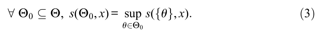
The s-value satisfies the following property:
By the property stated in Equation (3), the following property is entailed: for all , . Provided that the hypotheses are statements regarding to the parameter space, namely and , we have that: (1) ; (2) “”; and (3) “”. By the property stated in Equation (3), it is straightforward to show that the testing scheme based on the s-value satisfies monotonicity, intersection consonance and union consonance. The testing scheme based on the s-value does not satisfy invertibility, since the s-value allows us to maintain both hypotheses whenever the observed evidence is not strong enough against at least one of the null or the alternative hypotheses.
Some alternative Bayesian measures of evidence can be seen in Diniz, Pereira, Polpo, Stern, and Wechsler (2012). The authors studied some relationships between Bayesian and frequentist significance indices. It is beyond the scope of this article to compare the classical and Bayesian approaches.
Steps to Compute the s-Value
The steps to compute the s-value are the following:
Define the statistical model . Remember that represents the observable sample and contains random variables, namely
Define the null hypothesis and its related set
If required, define the alternative hypothesis and its related set
Compute the likelihood-ratio statistic
Compute
Compute
Compute
If required, compute
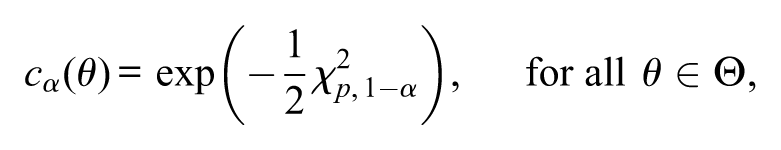
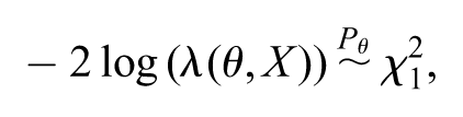
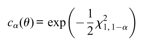
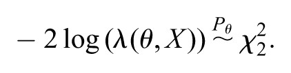
Step 5 is somewhat difficult to execute for some complex statistical models, since for those models the distribution of is not trivial and may depend on . In those cases, under regular conditions (Cox & Hinkley, 1974), the practitioner may apply the limiting distribution of , which is a chi-squared distribution with degrees of freedom, where (the Lebesgue measure). Then, Step 5 reduces to
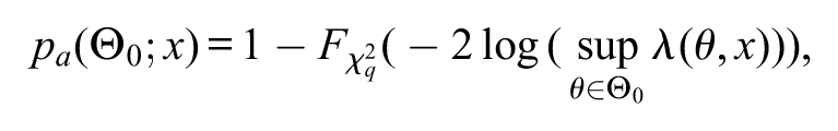
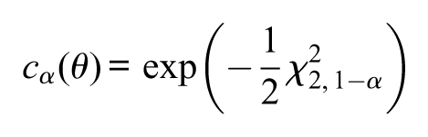
where is the quantile of a chi-squared distribution with degrees of freedom. This approximation reduces the complexity, since does not depend on . Under this asymptotic approximation, the “asymptotic”s-value, denoted by , reduces simply to
where is the cumulative distribution of a chi-squared distribution with degrees of freedom and is the natural logarithm function. If , then the asymptotic p-value (i.e., the asymptotic approximation for the p-value) based on the likelihood-ratio statistic coincides with the above asymptotic s-value. Nevertheless, if , the asymptotic p-value and asymptotic s-value will probably differ from each other. In the asymptotic p-value, the degree of freedom of the chi-squared distribution varies with the dimension of ; more precisely, the asymptotic p-value based on the likelihood-ratio statistic is
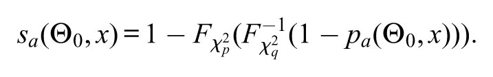
where , with . That is, the cumulative distribution function varies with the chosen null hypothesis, whereas for the s-value does not vary with the chosen null hypothesis. Patriota (2013, 2014) showed that the asymptotic s-values and p-values (based on the likelihood-ratio statistic) are connected through the following relation:
That is, from a p-value (based on the likelihood-ratio statistic) we can compute the s-value via the above formulae. If , then .
Numerical Examples
In this section, the s-value is applied for univariate and bivariate normal distributions. We consider known variances (and covariances) to maintain the simplicity. All required steps are computed.
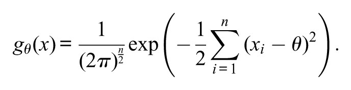
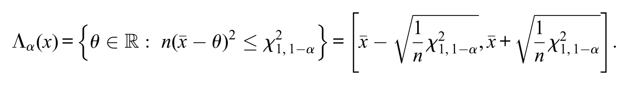
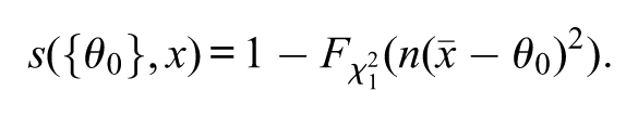
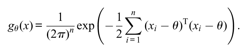
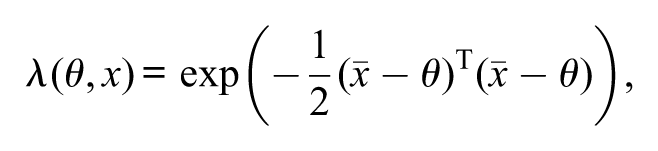
Example 1.(Normal distribution, variance known: z test) Let be a sample from a normal distribution with population mean and variance . Let be the null hypothesis of interest. The statistical model is , where and
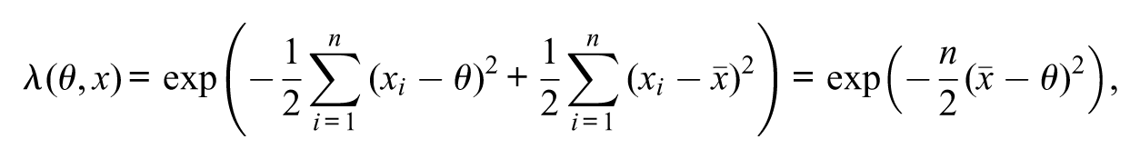
The likelihood-ratio statistic is
where is the maximum likelihood estimate for . It is known that
where the symbol “” means “follows a chi-squared distribution with degrees of freedom, under the law .” Then,
and
The quantity coincides with the normal -quantile , for instance, for , we have . That is, in this example, is the usual -confidence interval for the population mean.
Let be the null hypothesis of interest. The s-value is computed by finding the -value such that the border of the observed confidence interval is . The solution is
As aforementioned, for this simple null hypothesis, the s-value is precisely the p-value based on the likelihood-ratio statistic and coincides with the famous z-test.
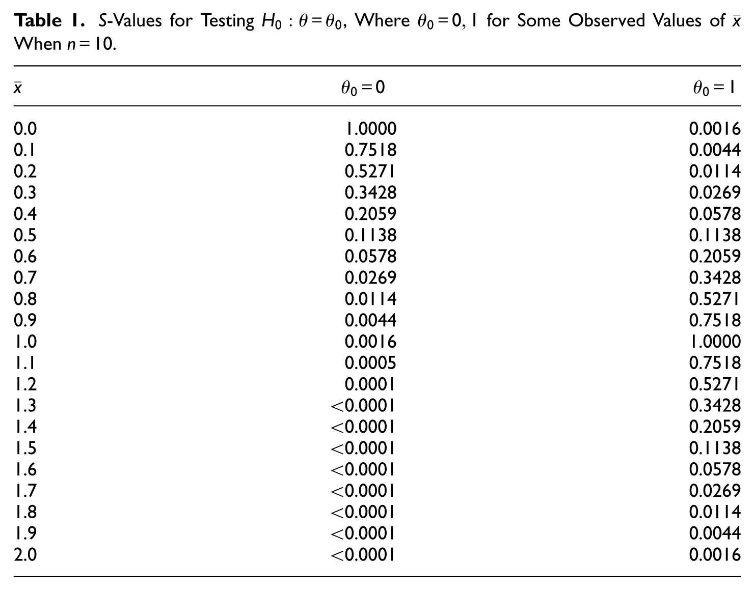
Table 1
depicts numerical s-values to illustrate the univariate normal distribution example for and . The null hypothesis is , where .
S-Values for Testing , Where for Some Observed Values of When .
0.0
1.0000
0.0016
0.1
0.7518
0.0044
0.2
0.5271
0.0114
0.3
0.3428
0.0269
0.4
0.2059
0.0578
0.5
0.1138
0.1138
0.6
0.0578
0.2059
0.7
0.0269
0.3428
0.8
0.0114
0.5271
0.9
0.0044
0.7518
1.0
0.0016
1.0000
1.1
0.0005
0.7518
1.2
0.0001
0.5271
1.3
<0.0001
0.3428
1.4
<0.0001
0.2059
1.5
<0.0001
0.1138
1.6
<0.0001
0.0578
1.7
<0.0001
0.0269
1.8
<0.0001
0.0114
1.9
<0.0001
0.0044
2.0
<0.0001
0.0016
Example 2.(Bivariate normal distribution, with known variances and covariances) Let be a sample from a bivariate normal distribution with population mean and covariance-variance matrix . The statistical model is , where and
The likelihood-ratio statistic is
where is the maximum estimate for , where and are the sample averages of the bivariate sample. Observe that, here . It is also known that
Then,
and
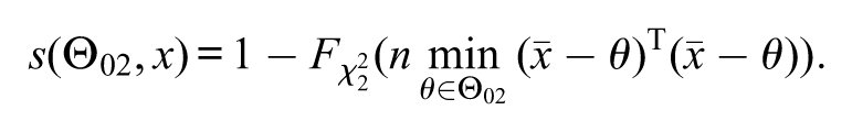
Null Hypothesis 1:Let be the null hypothesis of interest, where is a given vector; then . The s-value is computed by finding the -value such that the border of the observed confidence interval is . The solution is (which is also equal to the p-value based on the likelihood-ratio statistic)
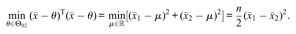
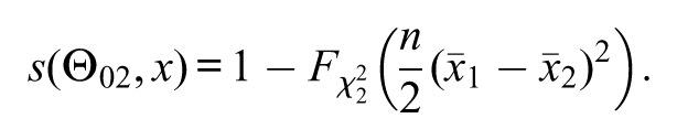
Null Hypothesis 2:Let be the null hypothesis of interest, then . The s-value is computed by finding the maximum -value such that
has at least one element. The solution is (which is not equal to the p-value based on the likelihood-ratio statistic)
Notice that
Then,
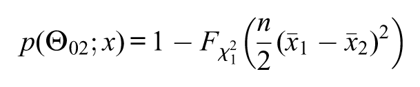
Recall that the p-value based on the likelihood-ratio statistic is
Table 2
presents numerical s-values to illustrate the bivariate normal distribution example for and covariance-variance matrix . The null hypotheses considered are and for which it is expected to find more evidence against than . The s-values were defined to hold this expected behavior. We purposely choose values for and such that p-values are problematic. The figures of
Table 2
show that all p-values fail to hold the logical condition for all sample, except for .
S-Values and p-Values for testing (the s-Values and p-Values Are Identical) and (the s-Values and p-Values Differ) for Some Observed Values of That Generate Problematic p-Values (Showing That p-Values Do Not Respect the Logical Consequence).a
(, )
s-value
p-value
s-value
p-value
(0.00, 0.00)
0.0
1.0000
1.0000
1.0000
1.0000
(0.05, –0.05)
0.1
0.9753
0.9753
0.9753
0.8231
(0.09, –0.11)
0.2
0.9039
0.9039
0.9048
0.6547
(0.14, –0.16)
0.3
0.7977
0.7977
0.7985
0.5023
(0.19, –0.21)
0.4
0.6697
0.6697
0.6703
0.3711
(0.23, –0.27)
0.5
0.5331
0.5331
0.5353
0.2636
(0.28, –0.32)
0.6
0.4049
0.4049
0.4066
0.1797
(0.33, –0.37)
0.7
0.2926
0.2926
0.2938
0.1175
(0.37, –0.43)
0.8
0.2001
0.2001
0.2019
0.0736
(0.42, –0.48)
0.9
0.1308
0.1308
0.1320
0.0442
(0.47, –0.53)
1.0
0.0813
0.0813
0.0821
0.0253
(0.51, –0.59)
1.1
0.0478
0.0478
0.0486
0.0139
(0.56, –0.64)
1.2
0.0269
0.0269
0.0273
0.0073
(0.61, –0.69)
1.3
0.0144
0.0144
0.0146
0.0037
(0.65, –0.75)
1.4
0.0073
0.0073
0.0074
0.0017
(0.70, –0.80)
1.5
0.0035
0.0035
0.0036
0.0008
(0.75, –0.85)
1.6
0.0016
0.0016
0.0017
0.0003
(0.79, –0.91)
1.7
0.0007
0.0007
0.0007
0.0001
(0.84, –0.96)
1.8
0.0003
0.0003
0.0003
0.0001
(0.89, –1.01)
1.9
0.0001
0.0001
0.0001
<0.0001
(0.93, –1.07)
2.0
<0.0001
<0.0001
<0.0001
<0.0001
The sample size is .
The behavior of p-values depicted in Tables 1 and 2 is not restricted to the examples where dispersion parameters are known. This feature happens also for unknown dispersion parameters, other test statistics, and other statistical models. Here, we consider likelihood-ratio statistics, since we are interested in comparing the p-value with the s-value. The distribution of is not trivial when the dispersion parameters are unknown and in order to avoid cumbersome computations, we consider only the case with known dispersion parameters.
Conclusion
This article discusses some conceptual and technical problems related to the null hypothesis statistical testing. The scientific and statistical hypotheses and the theoretical assumptions are connected by rules of inferences called modus ponnes and modus tollens, as studied in the section “Scientific and Statistical Hypotheses.” Unless the practitioner is totally certain of the theoretical assumptions, evidence to reject the null statistical hypothesis does not mean evidence to reject the scientific hypothesis, since the assumptions of a statistical model interfere in this process. Types of decisions in null hypothesis statistical testing depend on important assumptions that are not always made explicit. On one hand, if the practitioner considers the null and alternative statistical hypotheses are mutually exclusive and exhaustive, then procedures to accept–reject the null statistical hypothesis are justifiable (e.g., Neyman–Pearsonian and Bayesian procedures). On the other hand, if the practitioner considers that the null and alternative statistical hypotheses are mutually exclusive but not exhaustive, then procedures to reject the null statistical hypothesis are preferable (e.g., Fisherian procedures or some other procedures that do not use a belief measure that excludes all possibilities outside the null or alternative hypotheses), since a third option “” must be taken into account. A statistical procedure developed under one assumption will certainly fail to be appropriated under the other, therefore an extra caution must be taken when comparing different statistical procedures (classical vs Bayesian). By construction, p-values do not respect the following logical reasoning: if , then p-value() p-value(). That is, the practitioner must not use the p-value to extrapolate the inference made for to . This is not a defect in the classic statistical reasoning, because s-values do respect this logic and can be employed in the place of p-values. Asymptotic versions of s-values are simpler to compute than p-values. S-values can be used as a complementary measure of evidence and, as any other statistical measure, some care is needed when using it to make inferences; rules of thumb must be avoided, the inferential conclusions must be always complemented with other statistical tools.
My personal view is that models are useful tools, they can be adequate or inadequate in specific contexts. As for null hypotheses, they can be compatible or incompatible with the observed data; their degree of (in)compatibility with the observed data can be verified through measures of evidence (p-values, s-values, etc.). Statistical analyses have hard philosophical issues that should not be taken for granted, namely: translation problems, meaning of uncertainty, domain of applicability of each method, underlying (philosophical, scientific, logical, and statistical) principles and so on. My impression is that science would be more trustful if these issues were taken seriously into account in the statistical analyses. For instance, a p-value (or any other quantitative measure of evidence) smaller than a certain threshold (e.g., 0.05) should not be used directly to reject a scientific hypothesis without further investigations regarding model assumptions, test statistics, sample size, scientific relevance, rules of inferences, adopted principles, and so on.
Footnotes
Acknowledgements
The author thanks Prof. Dr. Denis Cousineau, Dr. Jonatas Eduardo Cesar, and two anonymous referees for their valuable comments and suggestions that led to an improved version of this article.
Declaration of Conflicting Interests
The author(s) declared no potential conflicts of interest with respect to the research, authorship, and/or publication of this article.
Funding
The author(s) disclosed receipt of the following financial support for the research, authorship, and/or publication of this article: The author gratefully acknowledges grant from FAPESP (2014/25595-0, Brazil).
Notes
References
1.
AtkinsonA. C. (1985). Plots, transformations and regression: An introduction to graphical methods of diagnostic regression analysis. Oxford, England: Oxford University Press.
2.
BergerJ. O.SellkeT. (1987). Testing a point null hypothesis: The irreconcilability of p values and evidence. Journal of the American Statistical Association, 82, 112-122.
3.
BollenK. A. (2002). Latent variables in psychology and the social sciences. Annual Review of Psychology, 53, 605-634.
4.
CookR. D. (1977). Detection of influential observation in linear regression. Technometrics, 19, 15-18.
5.
CookR. D. (1986). Assessment of local influence (with discussion). Journal of the Royal Statistical Society, Series B, 48, 133-169.
6.
CoxD. R. (1977). The role of significant tests (with discussion). Scandinavian Journal of Statistics, 4, 49-70.
DempsterA. P. (1968). A generalization of Bayesian inference. Journal of the Royal Statistical Society, Series B, 30, 205-247.
9.
DinizM.PereiraC. A. B.PolpoA.SternJ. M.WechslerS. (2012). Relationship between Bayesian and frequentist significance indices. International Journal for Uncertainty Quantification, 2, 161-172.
10.
FisherR. A. (1922). On the mathematical foundations of theoretical statistics. Philosophical Transactions of the Royal Society of London, Series A, 222, 309-368.
11.
FisherR. A. (1935). The logic of inductive inference. Journal of the Royal Statistical Society, Series B, 98, 39-82.
12.
FisherR. A. (1955). Statistical methods and statistical induction. Journal of the Royal Statistical Society, Series B, 17, 69-78.
13.
GonzálezJ. A.CastroL. M.LachosV. H.PatriotaA. G. (2016). A confidence set analysis for observed samples: a fuzzy set approach. Entropy, 18, 211.
14.
HájekA. (2008). Arguments for-or-against-probabilism?British Journal for the Philosophy of Science, 59, 793-819.
15.
HubbardR.BayarriM. J.BerkK. N.CarltonM. A. (2003). Confusion over measures of evidence (p’s) versus errors (α’s) in classical statistical testing. The American Statistician, 57, 171-182.
16.
IzbickiR.EstevesL.G. (2015). Logical consistency in simultaneous statistical test procedures. Logic Journal of IGPL. Advance online publlication. doi:10.1093/jigpal/jzv027
17.
KadaneJ. B. (2011). Principles of uncertainty. Boca Raton, FL: Chapman & Hall/CRC Press; 2011.
18.
KempthorneO. (1976). Of what use are tests of significance and tests of hypothesis. Communications in Statistics—Theory and Methods, 8, 763-777.
19.
LavineM.SchervishM. J. (1999). Bayes factors: What they are and what they are not. The American Statistician, 53, 119-122.
20.
LehmannE. L.CasellaG. (1998). Theory of point estimation (2nd ed.). New York, NY: Wiley.
21.
LehmannE. L.RomanoJ. P. (2005). Testing statistical hypotheses (3rd ed.). New York, NY: Springer.
22.
McCullaghP. (2002). What is a statistical model. Annals of Statistics, 30, 1225-1310.
23.
MayoD. G.CoxD. R. (2006). Frequentist statistics as a theory of inductive inference. In RojoJ. (Ed.), Optimality: The second Erich L. Lehmann Symposium. Lecture Notes–Monograph Series (Vol. 49, pp. 77-97). Beachwood, OH: Institute of Mathematical Statistics.
24.
MayoD. G.SpanosA. (2006). Severe testing as a basic concept in a Neyman-Pearson philosophy of induction. British Journal for the Philosophy of Science, 57, 323-357.
25.
PatriotaA. G. (2013). A classical measure of evidence for general null hypotheses. Fuzzy Sets and Systems, 233, 74-88.
26.
PatriotaA. G. (2014). Uma medida de evidência alternativa para testar hipóteses gerais [An alternative evidence measure to test general hypotheses]. Ciência e Natura, 36, 14-22. Retrieved from http://www.ime.usp.br/patriota/medida_evi.pdf
27.
PatriotaA. G. (2015). A measure of evidence based on the likelihood-ratio statistics. Retrieved from http://arxiv.org/abs/1510.02950
28.
SchervishM. J. (1995). Theory of statistics. New York, NY: Springer.
29.
SchervishM. J. (1996). P values: What they are and what they are not. The American Statistician, 50, 203-206.
TrafimowD. (2003). Hypothesis testing and theory evaluation at the boundaries: Surprising insights from Bayess theorem. Psychological Review, 110, 526-535.
32.
TrafimowD.MarksM. (2015). Editorial. Basic and Applied Social Psychology, 37, 1-2.