A Comparison of Methods for Estimating Relationships in the Change Between Two Time Points for Latent Variables

Abstract

Collection and analysis of longitudinal data is an important tool in understanding growth and development over time in a whole range of human endeavors. Ideally, researchers working in the longitudinal framework are able to collect data at more than two points in time, as this will provide them with the potential for a deeper understanding of the development processes under study and a much broader array of statistical modeling options. However, in some circumstances data collection is limited to only two time points, perhaps because of resource limitations, issues with the context in which the data are collected, or the nature of the trait under study. In such instances, researchers may still want to learn about complex relationships in the data, such as the correlation between changes in latent traits that are being measured. However, with only two data points, standard approaches for modeling such relationships, such as growth curve modeling, cannot be used. The current simulation study compares the performance of two methods for estimating the correlations among changes in latent variables between two points in time, the two-wave latent change score model and the latent difference factor model. Results of the simulation study showed that both methods yielded generally accurate estimates of the correlation between changes in a latent trait, with relatively small standard errors. Estimation bias and standard errors were lower with larger samples, larger factor loading magnitudes, and more indicators per factor. Further comparisons between the methods and implications of these results are discussed.

Keywords

longitudinal data change scores latent variable modeling

Many researchers working in human development are interested in assessing change over time in one or more psychological constructs, such as mathematics aptitude (Purpura & Logan, 2015), vocabulary development (Mohammed, Majid, & Abdullah, 2016), critical thinking (Ralston & Bays, 2015), and cognition (Budiman, Halim, Mohd Meerah, & Osman, 2014). Perhaps the most effective method for examining such developmental issues involves the use of longitudinal study designs in which a sample of individuals is followed for a period of time, and their performance on one or more constructs of interest is measured multiple times. Higher frequency of the data collection is generally preferred by the researchers using such longitudinal designs (e.g., Selig & Preacher, 2009). However, in some situations where the cost of data collection is very high, or maintaining contact with study participants is logistically challenging, data may only be collected at two points in time. In addition, even for studies in which more than two occasions of data will eventually be collected, the researcher may wish to explore patterns in the initial two time points that are collected, while they wait for the rest of the data collection to conclude.

When examining two occasion data, the researchers may be particularly interested in latent variables, such as cognition or motivation. While there are various definitions of latent variables, latent variables are generally viewed as hypothetical and immeasurable constructs representing the underlying cause or true scores of observed scores. Thus, latent variables are instrumental for gaining insights into important psychological phenomena. Of interest in the current study is understanding how change in one such construct is related to change in another. For data with more than two time points, a growth curve model (GCM) has been a commonly used an analytic tool. In GCM, changes for each of the constructs are modeled as latent variables, and then the correlation in these change factors for two or more constructs can be estimated. However, for the data with only two time points, the use of GCM is not possible because there are not sufficient degrees of freedom with which to fit the model.

Recently, a model for estimating the relationships in change over time for latent variables with two time points has been suggested in the form of the two-wave latent change score (2W-LCS) model (Henk & Castro-Schilo, 2016). In their article, Henk and Castro-Schilo (2016) described the 2W-LCS in detail and demonstrated it with several empirical examples. However, the method was not studied using a Monte Carlo simulation approach with known model parameters in order that its performance under a variety conditions and its performance in general could be assessed. Accordingly, one purpose of the current study is to extend the literature on the 2W-LCS model by examining its performance using a simulation study. Additionally, we will compare it with an alternative approach to modeling relationships in change over time, using a difference score latent modeling approach (latent difference factor [LDF]) introduced here. In the following sections, we present a brief review of the literature on latent change score analysis, followed by a description of the two models under investigation. The simulation methodology used in the current study is then presented, followed by an examination of the results of the simulation study, and an analysis of empirical data using the two methods examined here. Finally, the results of the current study are discussed in the context of literature in the field.

Modeling Relationships in Change for Latent Variables

As noted above, one of the most common approaches for modeling change in latent variables over time, and one that allows for estimation of the relationship of change for two (or more) different latent variables, is GCM. However, when data from only two time points are available, this approach cannot be used, as there is not sufficient information available to estimate all of the model parameters. Other approaches that have been suggested in the literature for use with two occasion data include the latent change score (LCS) model (Selig & Preacher, 2009) and the two-wave panel model (2WPM) described by Little, Preacher, Selig, and Card (2007). Each of these models presents the researcher with a powerful set of tools for modeling change over time with latent variables, and each can be used with only two time points, unlike GCM.

Selig and Preacher’s (2009) model is based on earlier work in the area of latent difference scores, in particular that of McArdle and Nesselroade (1994). In its simplest form for two points in time, this approach models the value of a variable, x, at time t as being a function of the variable at the previous time (t− 1) and the latent change in x. More specifically,

x_{t} = x_{t - 1} + Δ x_{t},

where $Δ x_{t} = β_{t - 1} x_{t - 1}$ and $β_{t - 1}$ is the effect of previous level of x on the change in x.

In their work, Selig and Preacher (2009) describe the utility of this model for estimating indirect effects from a mediation perspective, though the model framework allows for estimation of other effects as well. The relationship between the two time points would be captured by $β_{t - 1}$ . Selig and Preacher recommend having at least four time points available when estimating the parameters for model (1), and thus, this model has limited applicability to the data with only two data points, which is the focus of the current study.

In their recent review of the literature, Henk and Castro-Schilo (2016) discussed a second modeling paradigm, the 2WPM (Little et al., 2007), in the context of examining theories of change. However, as Henk and Castro-Schilo noted, this approach does not allow for a direct estimation of the relationship in change over time for the variables involved. Consider the example in which two variables are measured at two points in time, and we are interested in how each changes over time, as well as in characterizing the impact of the value at the first time point for one variable on the value of the other variables at the second time point. For the 2WPM this model would take the following form:

\begin{array}{l} y_{2} = β_{y 1} y_{1} + γ_{x 1} x_{1}, \\ x_{2} = β_{x 1} x_{1} + γ_{y 1} y_{1}, \end{array}

where $β_{y 1}$ is the autoregressive parameter linking the value of the Time 1 measurement for y with the Time 2 measurement for y; $β_{x 1}$ is the autoregressive parameter linking the value of the Time 1 measurement for x with the Time 2 measurement for x; $γ_{x 1}$ is the cross-lagged regression parameter linking the value of the Time 1 measurement for x with the Time 2 measurement for y; and $γ_{y 1}$ is the cross-lagged regression parameter linking the value of the Time 1 measurement for y with the Time 2 measurement for x.

Note that in this model there is not a parameter estimating a relationship in the change in y (from $y_{1}$ to $y_{2}$ ) with the change in x (from $x_{1}$ to $x_{2}$ ). Therefore, while certainly useful in many contexts, the 2WPM may not prove particularly helpful when the primary research interest involves measuring the relationship between change in one variable and change in another.

Two-Wave Latent Change Score Model

Henk and Castro-Schilo (2016) described a new approach for estimating the relationship between changes in two variables, the 2W-LCS model. This model was demonstrated with an empirical example and the types of models that could be fit with it were also outlined. Nonetheless, its performance under known conditions, using a Monte Carlo simulation study design, has not been assessed. This assessment, therefore, is one of the major goals of the current study.

The measurement portion of the 2W-LCS at time point t is expressed as

y_{i t} = τ + Λ η_{i t} + ε_{i t},

where $y_{it}$ is the vector of measurements on p variables for individual i at time t; $τ$ is the time-invariant intercepts; $Λ$ is the time invariant loadings; $η_{it}$ is the factor score for individual i at time t; and $ε_{it}$ is the error for individual i at time t.

It is assumed that $ε_{it} ~ N (0, θ),$ with $θ$ being a $p \times p$ symmetric tridiagonal matrix with factor variances on the diagonal. The structural portion of the 2W-LCS takes the following form:

η_{i 2} = η_{i 1} + Δ_{i},

where $η_{i 1}$ is the factor score for person i at Time 1; $η_{i 2}$ is the factor score for person i at Time 2; $Δ_{i} = κ + B Δ_{i} + ς_{i}$ is the vector of latent change scores for person i; $κ$ is the vector of intercepts; $B$ is the matrix of regression coefficients among change score, with 0 diagonal elements reflecting that no change factor predicts itself; $ς_{i}$ is the vector of random error assumed to be distributed N(0, $ψ$ ); $ψ$ is the diagonal matrix of factor and residual variances. It is assumed that factor loadings and intercepts are invariant across time, t.

In the context of understanding relationships between change scores for latent variables, the focus will be placed on $B$ in Equation (4). The elements of this matrix serve as the measures of the relationships in change scores for all of the latent variables included in the model. In the simple case where there are two such variables, $ϕ$ and $η,$ the coefficient $B_{Δ ϕ, Δ η}$ expresses the relationship between change in $ϕ$ ( $Δ ϕ$ ) and change in $η$ ( $Δ η$ ). Henk and Castro-Schilo (2016) note that when interpreting the meaning of $B$ in the context of a particular research problem, it is also important for the researcher to fit individual univariate change models for each factor separately, in order to ascertain whether and what type of change in factor means was found to be present for the construct. Knowing whether the mean of each latent variable changed over time, and if so, in what direction (positive or negative) that change occurred will help the researcher to accurately interpret the coefficients in $B$ .

The 2W-LCS model appears in Figure 1. In this example, there are two factors measured at two time points using three indicators each. The latent variables Delta_1 and Delta_2 represent the change in F1 and F2, respectively. The relationship between these factor changes is denoted by the path DELTA_F1 WITH DELTA_F2. Note that the loadings linking the factors with each indicator are constrained to be the same across the two times. For example, the loading for F1_T1 with Y2_T1 is equal to the loading linking F1_T2 and Y2_T2.

Figure 1.

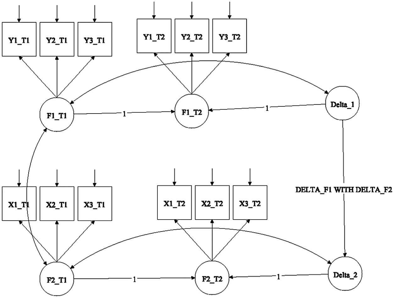
2W-LCS path model.

Latent Difference Factor

An alternative approach to estimating the relationship between changes in latent variables involves the use of the LDF approach. LDF conceptualizes the change over time in a latent variable, and more specifically its indicators, as a latent construct of its own. Thus, if we are presented with two latent variables, $ϕ$ and $η$ , measured at two points in time, then the change in each of these, $Δ ϕ$ and $Δ η$ , respectively, represent unique factors of their own. Given this fact, it is possible to estimate the correlation between the factors $Δ ϕ$ and $Δ η$ and thereby assess how change in $ϕ$ is related to change in $η .$

In order to examine how the LDF model works, assume the following measurement models for each factor at time t:

y_{it} = τ_{ϕ t} + Λ_{ϕ t} ϕ_{it} + ε_{iyt},

x_{it} = τ_{η t} + Λ_{η t} η_{it} + ε_{ixt},

where $y_{it}$ is the vector of observed indicators for factor $ϕ$ for person i at time t; $τ_{ϕ t}$ is the vector of intercepts for $ϕ$ at time t; $Λ_{ϕ t}$ is the matrix of loadings for $ϕ$ at time t; $ϕ_{it}$ is the factor score on $ϕ$ for person i at time t; $ε_{ity}$ is the vector of errors for person i at time t for the y indicators; $x_{it}$ is the vector of observed indicators for factor $η$ for person i at time t; $τ_{η t}$ is the vector of intercepts for $η$ at time t; $Λ_{η t}$ is the matrix of loadings for $η$ at time t; $η_{it}$ is the factor score on $η$ for person i at time t; and $ε_{itx}$ is the vector of errors for person i at time t for the x indicators.

We can assess the change over time for a given indicator variable, $y_{i}$ , using a difference score

Δ y_{i} = y_{i 2} - y_{i 1} .

Likewise, it is possible to express the change in factor score $ϕ$ as

Δ ϕ_{i} = ϕ_{i 2} - ϕ_{i 1} .

In a similar fashion, we can express the change in the indicators of $η$ and the factor itself as

Δ x_{i} = x_{i 2} - x_{i 1},

Δ η_{i} = η_{i 2} - η_{i 1} .

Finally, combining the results in Equations (7) through (10), we can estimate the measurement models for the difference factors using the differences in (7) and (9) as the indicators, such that

Δ y_{i} = τ_{Δ ϕ} + Λ_{Δ ϕ} ϕ_{Δ i} + ε_{Δ iy},

Δ x_{i} = τ_{Δ η} + Λ_{Δ η} η_{Δ i} + ε_{Δ ix} .

Finally, the relationship between $Δ ϕ$ and $Δ η$ can be estimated in a structural model as the correlation between these two difference factors.

The following steps are used when fitting the LDF model:

Assess the fit of each factor separately at each point in time using confirmatory factor analysis (CFA). The individual factor models (Equations 5 and 6) must yield good fit to the data at each time point in order for LDF model fitting to continue.

Assuming that good fit is found in Step 1, calculate difference scores for each indicator variable for each factor.

Fit the difference factor models (Equations 11 and 12) for each latent variable separately, using CFA. The difference factor models must yield good fit for each latent variable in order for LDF model fitting to continue.

Presuming that the difference models fit in Step 3, estimate the correlation between the difference factors using a structural equation modeling approach.

The path diagram for the LDF model appears in Figure 2. This model represents the same problem as that addressed in Figure 1, namely, the estimation of the relationship in change scores for Factors 1 and 2 between Times 1 and 2. In the case of the LDF, a difference score is calculated for each indicator for each factor, leading to DY_1, DY_2, DY_3, DX_1, DX_2, and DX_3. These difference scores then serve as the indicators for the difference factors, DF_1 and DF_2. The correlation between these difference factors is then estimated, providing an indication of the extent to which the changes in the latent traits are related to one another.

Figure 2.

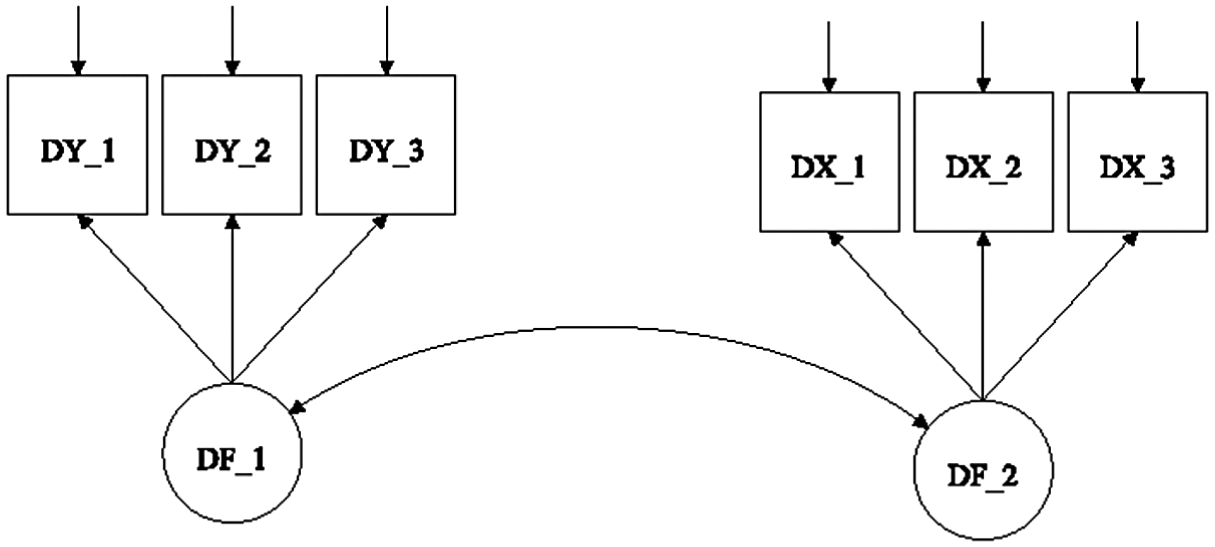
LDF path model.

The LDF model can easily incorporate a variety of additional structural model forms, such as the multiple indicators multiple causes (MIMIC) model, factor model invariance testing, and assessment of structural relationships among change factors for several latent traits, among others. In addition, it is possible to estimate the means of the latent difference variables for different groups within the population (e.g., males and females), and to compare these means statistically in order to ascertain whether one group experienced more change over time than another. For example, because change over time in a factor is representing itself as a latent variable, it would be possible to determine whether change over time differs for males and females, using a MIMIC model. In addition, using model invariance testing, it would be possible to ascertain whether the relationships (as measured by $Λ_{Δ ϕ}$ ) between the change in individual indicators ( $Δ y$ ) and their latent change factor ( $ϕ_{Δ}$ ) are equivalent across groups (e.g., genders). Likewise, structural models could be fit assessing the nature of relationships among change factors. Some of these applications of the method will be demonstrated below.

Study Goals

The current study has two primary goals. First, it is designed to extend the work of Henk and Castro-Schilo (2016) by examining the performance of the 2W-LCS model under controlled conditions using a simulation study. As noted above, this approach has been shown to be promising using real empirical data, but has not yet been assessed under such controlled conditions. Second, this study serves as an introduction of a new approach for assessing the nature and direction of change in latent variables, the LDF model. This model has also not been studied under controlled simulation conditions previously, which the current study is designed to address. As described below, the study has been designed to assess and compare the performance of these methods under a variety of conditions designed to mirror what might be seen in actual practice, in terms of sample sizes, number of indicators, factor loading magnitudes, and interfactor correlations.

Given that virtually no simulation work has been done previously with these methods, it is not possible to develop strong hypotheses regarding what the current study will show. However, some initial guesses as to what might be expected in terms of results can be posited here, based on prior research. First, we anticipate that given its relatively simpler structure, the LDF model may have less difficulty converging than will the 2W-LCS when the sample size and number of indicators are small. On the other hand, for larger samples and more indicators, we might expect the 2W-LCS model to yield somewhat smaller standard errors for the estimates, because it directly accounts for the error terms of the individual indicators at each time rather than the combined errors present in the LDF model. Finally, we anticipate that both methods will yield relatively unbiased estimates of the correlation between changes in the latent traits, and that for both approaches the standard errors will be lower with larger samples, more indicators, and stronger relationships between the individual indicators and their latent traits.

Method

In order to address the research goals described above, a Monte Carlo simulation study design was used, with 1,000 replications per combination of conditions, which are described below. The data were generated from a two-factor model with two time points, whereby each factor exhibited simple structure, that is, each indicator variable was associated with only one factor. The indicators were generated from the N(0, 1) distribution, as were the error terms and factors. The mean change over time for the factors was simulated to be 1 SD. Data generation and analysis were carried out using the R software package (R Development Core Team, 2015), as well as Mplus, version 7.11 (Muthén & Muthén, 2015). The manipulated study settings are described below.

Sample Size

Sample sizes were simulated to be 100, 200, 300, 400, 500, 600, 700, 800, 900, and 1,000. These values were selected because they represent a range from what would be considered a small sample in the context of factor analysis (100) to a large sample (1,000).

Number of Indicators per Factor

Four conditions for number of indicators per factor were simulated: 3, 5, 10, and 15. These values were selected to reflect a range of cases, from a minimal number needed to ensure no problems with model identification (3) to a fairly large number (15). The number of indicators was the same for each factor.

Factor Loading Magnitude

The factor loadings were simulated to be 0.5, 1, and 1.5. For a given setting (e.g., 1), loadings for all of the indicator variables were simulated to be the same. In addition, as noted above all of the indicators were simulated from the N(0,1) distribution, and the latent variables were simulated to reflect pure simple structure. The loading values themselves were selected to represent the case where the factor structure was fairly weak (0.5) to the situation where it was quite strong (1.5).

Correlation Between Factor Change Scores

The correlation between the changes in latent traits was simulated to be either 0.32 or 0.68. These values represent what might be thought of as moderate and large correlation values (Cohen, 1988).

Outcomes

The study outcomes included convergence rates, correlation estimation bias, the standard error of the correlation estimates, and the mean squared error (MSE) of the estimates. Correlation estimate bias is calculated as

Bias = ρ - {\hat{ρ}}_{r},

where $ρ$ is the population correlation between factor change scores; ${\hat{ρ}}_{r}$ is the estimated correlation between factor change scores for simulation replication r.

The standard error of the correlation estimates was

SE = \frac{\sum_{r = 1}^{R} {({\hat{ρ}}_{r} - \bar{ρ})}^{2}}{R},

where $\bar{ρ}$ is the mean correlation across the R replications; R is the number of replications.

The MSE was calculated to be

MSE = Bia s^{2} + S E^{2} .

For each of these outcomes, analysis of variance (ANOVA) was used in conjunction with the $η^{2}$ effect size to identify the manipulated study factors, and their interactions, that were related to each of the three outcome variables. Only those main effects and interactions that were statistically significant, and that accounted for at least 10% ( $η^{2} = 0.1$ ) of the variance in the outcome variable, were considered for discussion in the results.

Results

Convergence Rates

Convergence rates for both methods were 100% across conditions, except for small sample sizes with few indicators, low factor loadings, and a smaller correlation between the factors. Specifically, the convergence rate for LDF for an interfactor correlation of 0.32 with factor loadings of 0.5, 3 indicators, and sample sizes of 100, 200, and 300 was 0.96, 0.973, and 0.996, respectively. For the same combinations of conditions, the convergence rates of 2W-LCS were 0.987, 1.000, and 1.000, respectively. In all other cases, the convergence rates were 1.000.

The Mean Square of the Error

The results of the ANOVA showed that for MSE, the interaction of the estimation method by the number of indicator variables by the factor loading magnitude was the highest order statistically significant term, with $η^{2}$ of at least 0.1 ( $F_{6, 159} = 5.826, p = . 00002, η^{2} = 0.180$ ). Figure 3 displays the MSE by the estimation method, number of indicators, and indicator magnitude. MSE was largest for both methods when there were 3 indicators per factor and the factor loadings were 0.5. In this case, and for 5 indicators with loadings of 0.5, the MSE for LDF was somewhat larger than that of 2W-LCS. On the other hand, for the 10-factor condition with a loading of 0.5, the MSE for 2W-LCS was higher than for LDF. In all other cases, the two methods yielded comparable MSE values.

Figure 3.

Correlation estimate MSE by estimation method, number of factor indicators, and factor loading magnitude.

Bias

The ANOVA identified three statistically significant interactions to be associated with estimation bias, including estimation method by number of indicators ( $F_{3, 159} = 10.216, p = . 000003, η^{2} = 0.116$ ), estimation method by factor loading magnitude ( $F_{2, 159} = 48.278, p < . 000001, η^{2} = 0.378$ ), and estimation method by sample size ( $F_{9, 159} = 2.653, p = . 007, η^{2} = 0.131$ ). Figure 4 displays the bias in the correlation estimates by method and number of indicators. Across conditions, bias was always below 0.055, and was positive, meaning that both approaches overestimated the correlation between the changes in the factors. When 3 or 5 indicator variables were present, the LDF approach produced slightly more biased estimates than did 2W-LCS. On the other hand, for 10 and 15 indicators, estimation bias was lower for LDF than for 2W-LCS. For both methods, bias was lower when more indicators were present, such that for 15 indicators LDF yielded a bias result of approximately 0.008, whereas 2W-LCS had bias of approximately 0.024.

Figure 4.

Correlation estimate bias by estimation method and number of indicators.

Figure 5 includes correlation estimate bias by estimation method and factor loading magnitude. When the loadings were 0.5 in the population, bias was greater for the LDF approach than for 2W-LCS. On the other hand, for loading magnitudes of 1 and 1.5, bias was slightly greater for 2W-LCS. Estimation bias for both methods declined concomitantly with increases in the factor loading magnitude. Correlation estimation bias by sample size and estimation method appears in Figure 6. For both approaches, bias declined with increases in sample size. When N was 300 or less, LDF had lower biased estimates than did 2W-LCS. On the other hand, for all other sample sizes, 2W-LCS produced slightly less biased estimates than LDF.

Figure 5.

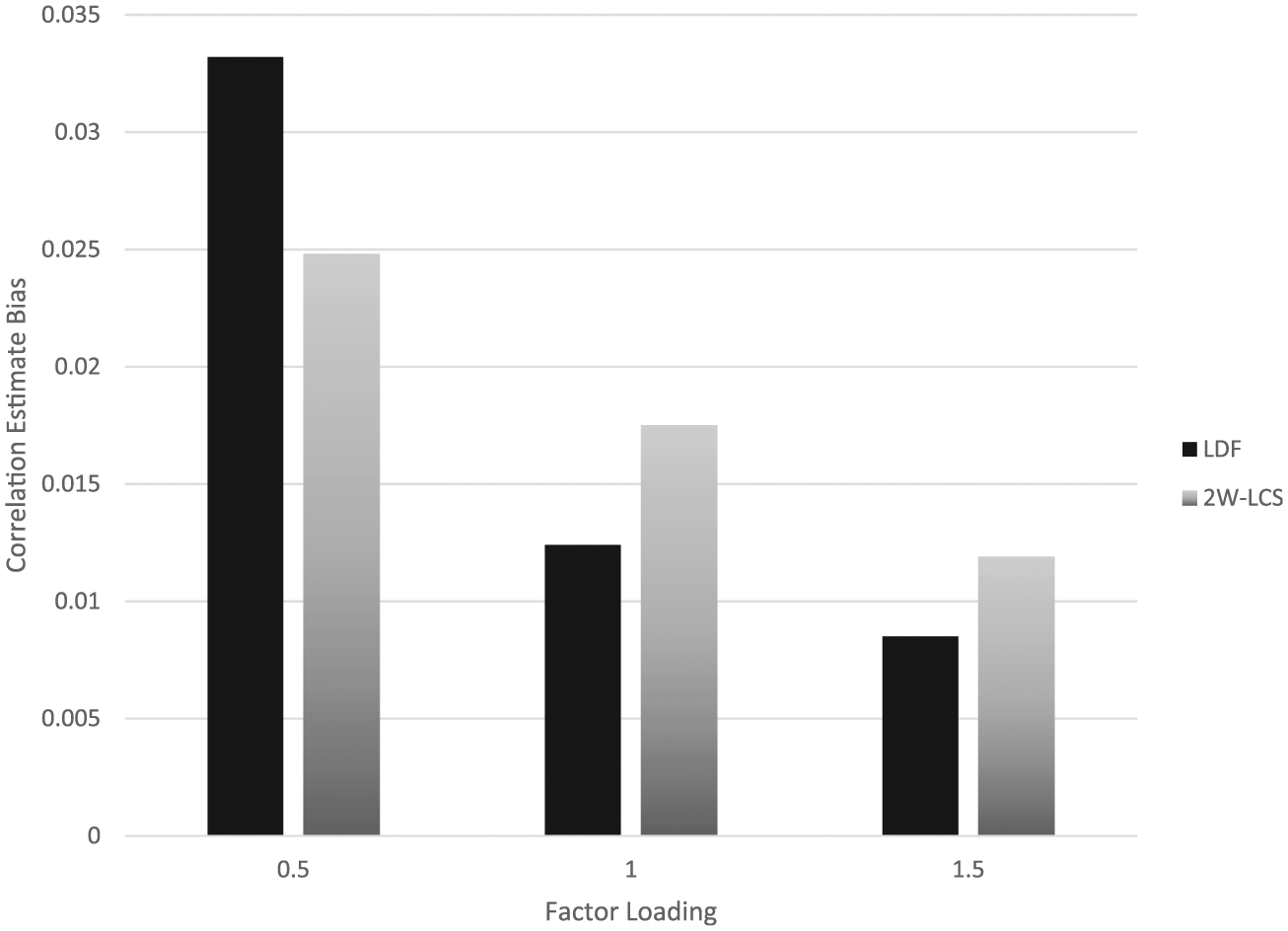
Correlation estimate bias by estimation method and factor loading magnitude.

Figure 6.

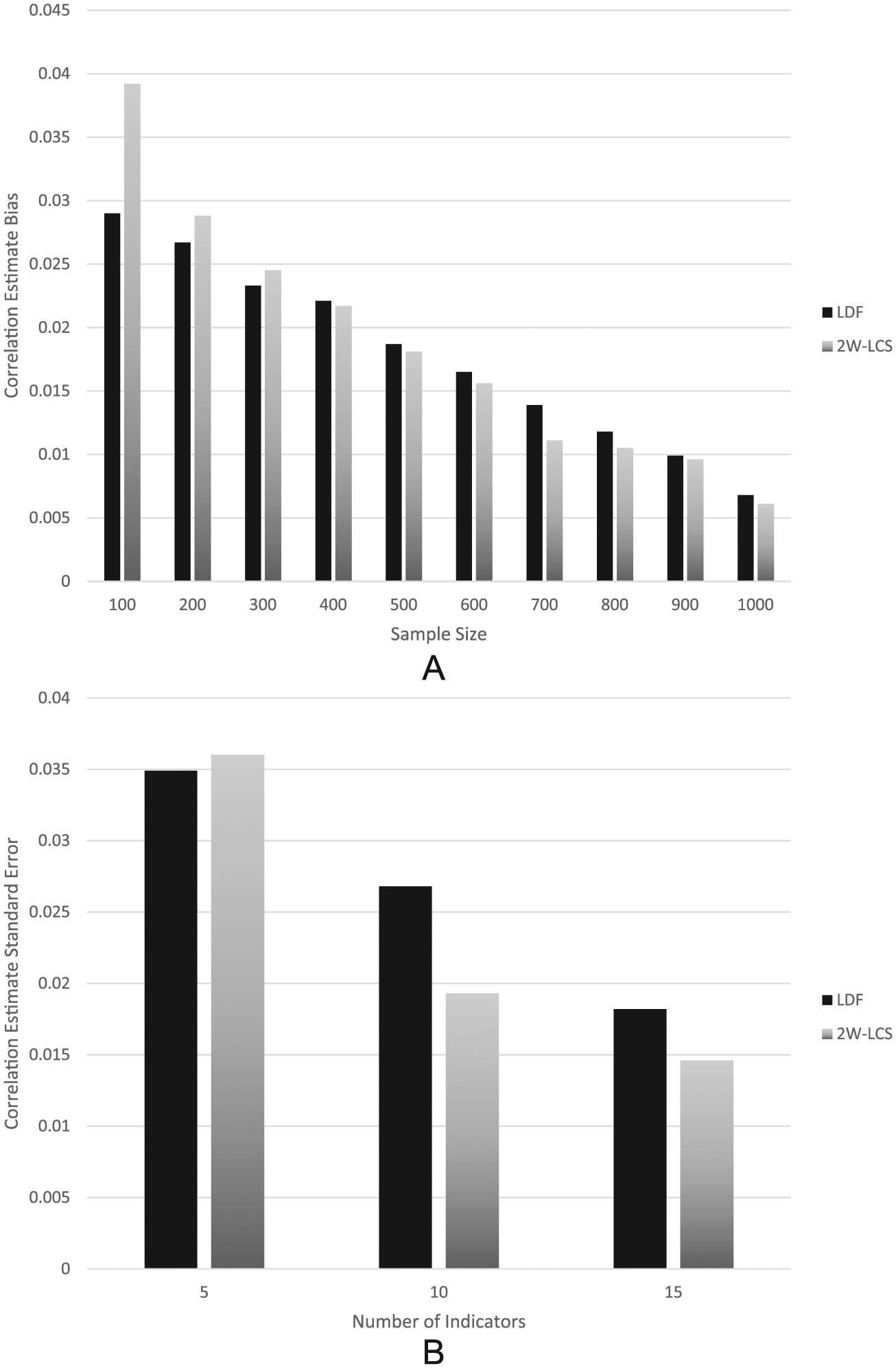
(A) Correlation estimate bias by estimation method and sample size. (B) Correlation Estimate Standard Error by Estimation Method and Number of Indicators.

Standard Error

The ANOVA showed that the interaction of estimation method by number of indicators ( $F_{3, 159} = 9.1, p = . 000014, η^{2} = 0.147$ ) and the interaction of estimation method by sample size ( $F_{9, 159} = 2.669, p < . 007, η^{2} = 0.131$ ) were both significantly related to the estimate standard error. Figure 6 includes the standard error of the correlation estimate by estimation method and number of indicators. The results show that for 3 and 5 indicators, the standard error of the 2W-LCS was slightly larger than that of LDF. However, for 10 and 15 indicators the 2W-LCS standard error was lower than that of LDF. For both methods, the standard error declined in value as the number of indicators per factor increased. Figure 7 displays the correlation estimate standard error by estimation method and sample size. For both LDF and 2W-LCS, the standard error declined as the sample size increased. In addition, across sample size conditions, the standard error was larger for LDF than for 2W-LCS, and this effect was greater at the smaller sample size conditions.

Figure 7.

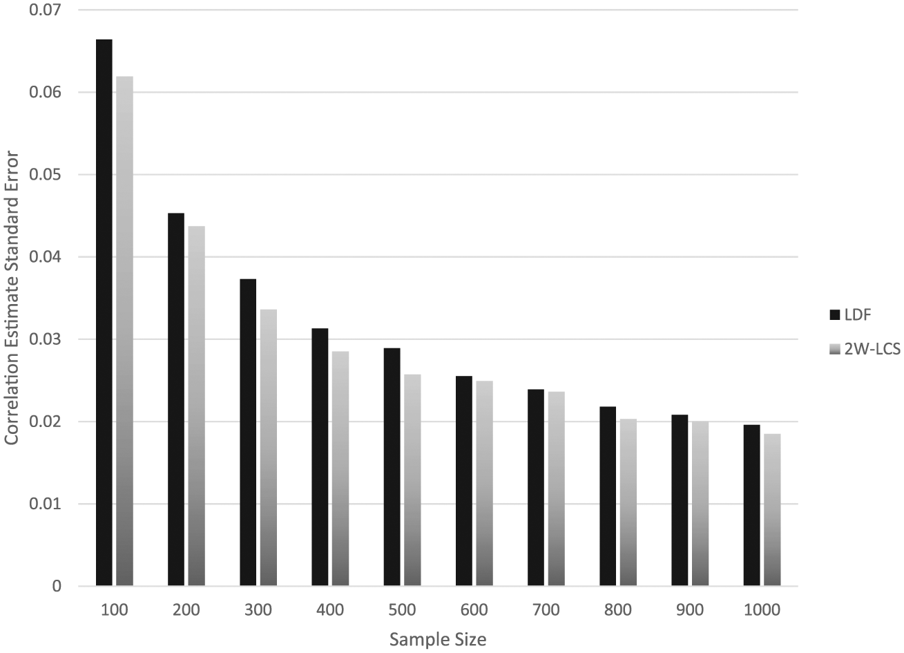
Correlation estimate standard error by estimation method and sample size.

Empirical Example

In order to demonstrate the use of LDF and 2W-LCS for assessing relationships in change over time for latent constructs, we consider a research example involving the longitudinal assessment of teacher provision of autonomy support in the classroom. In particular, 324 students responded to the Teacher as a Social Context (TASC) student-report scale (Belmont, Skinner, Wellborn, & Connell, 1992). This scale consists of three subscales: teacher provision of relatedness, teacher provision of autonomy support, and teacher provision of structure. Therefore, a three-factor CFA was fit to the data, as is described in more detail below. The scale is based on self-determination theory (Ryan & Deci, 2000), which is a major theory of motivation. These three instructional behaviors are deemed important to support students’ intrinsic motivation, engagement, and achievement.

The original scale included 54 items. Due to the available time allowed to collect the data by the school, a subset of 31 items from the original scale was used in the present study. The items are measured on a 5-point Likert-type scale (1 = Strongly disagree, 2 = Disagree, 3 = Not sure, 4 = Agree, and 5 = Strongly agree). Respondents were given the TASC at the beginning of fall semester and again in spring semester of the same school year. Students voluntarily participated in the study and several researchers were present to answer questions. The research question of interest was whether relationships existed among the change in the students’ perception of their teachers’ instructional practices, as reflected in the three constructs listed above. Each of these constructs can be represented by a factor in a latent variable model, and the researcher’s question can be addressed by estimating the correlations between the changes in the TASC factors over time, using both the LDF and 2W-LCS methods. As mentioned above, a three-factor CFA was fit to the data, in which each factor corresponded to one of the three TASC subscales: teacher provision of relatedness, teacher provision of autonomy support, and teacher provision of structure. All analyses were conducted using Mplus version 7.11 (Muthén & Muthén, 2015). The CFA model was fit using the robust weighted least squares (WLSMV estimator), with the difference factor indicators being the difference scores in the observed indicators for each of the factors of interest. Model fit was assessed using several model indices, including the chi-square goodness of fit test, comparative fit index (CFI), Tucker–Lewis index (TLI), root mean square error of approximation (RMSEA), and standardized root mean square residual (SRMR; Kline, 2016).

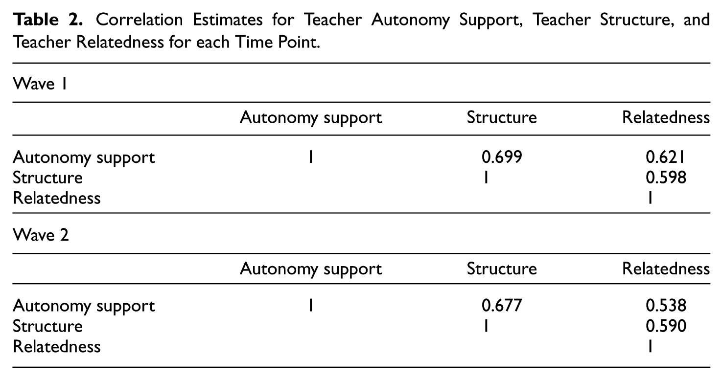
Table 1 includes fit indices for each of the models that were fit to the data. As noted above, in the process of fitting the LDF model, it is necessary to ensure that the hypothesized factor structure fits the data at each time point, independently. This was assessed with separate models at times 1 and 2, with the fit statistics appearing in Table 1. These results are all in keeping with what is generally considered to represent good fit (Kline, 2016; CFI > 0.95, TLI > 0.95, RMSEA < 0.05, SRMR < 0.08), with the exception of the chi-square test, which rejected the null hypothesis of good model fit. However, it is well known that this test is sensitive to sample size and may yield statistically significant results even when model fit is actually good (Kline, 2016). Given the model fit results, it was appropriate to proceed to fitting the LDF model. Again, the fit statistics for this model appear in Table 1, and indicate that the LDF model provided good fit to the data. Likewise, the 2W-LCS model also provided good fit to the data, with first statistic values slightly lower than those for the LDF model, but still indicating good model–data fit. Table 2 contains the correlations between the three factors of interest at each wave of data collection. These results demonstrate that at both measurement occasions, the factors exhibited correlations between 0.5 and 0.7.

Table 1.

Model Fit Indices for Example Data Analysis Models.

Model	CFI	TLI	RMSEA	SRMR	χ² (df)
Time 1 model	0.98	0.98	0.02	0.06	1021.785 (402)*
Time 2 model	0.98	0.97	0.03	0.05	1181.822 (402)*
LDF	0.96	0.95	0.04	0.06	1809.926 (402)*
2W-LCS	0.94	0.93	0.05	0.07	11743.2 (1,903)*

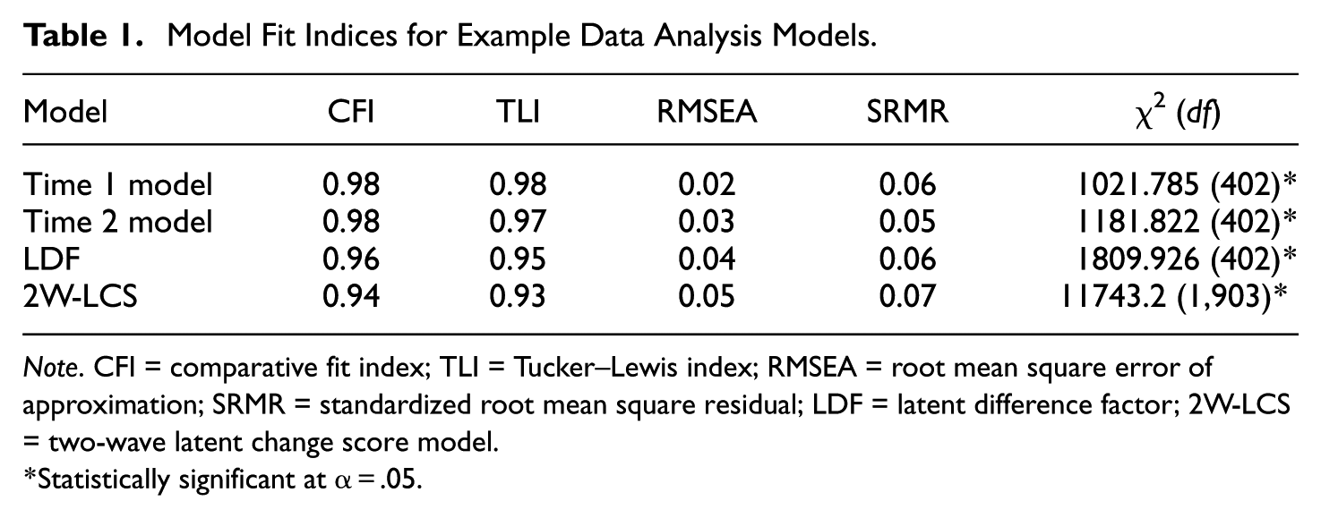
Note. CFI = comparative fit index; TLI = Tucker–Lewis index; RMSEA = root mean square error of approximation; SRMR = standardized root mean square residual; LDF = latent difference factor; 2W-LCS = two-wave latent change score model.

Statistically significant at α=.05.

Table 2.

Correlation Estimates for Teacher Autonomy Support, Teacher Structure, and Teacher Relatedness for each Time Point.

Wave 1
	Autonomy support	Structure	Relatedness
Autonomy support	1	0.699	0.621
Structure		1	0.598
Relatedness			1
Wave 2
	Autonomy support	Structure	Relatedness
Autonomy support	1	0.677	0.538
Structure		1	0.590
Relatedness			1

The correlation estimates among the change in factors appear in Table 3. From these results, we can see that the two methods yielded very similar estimates of the correlations among the latent traits. In particular, both approaches found that student perceptions of change in autonomy support were positively associated with their perceptions in structure, and essentially not related to their perceptions of changes in relatedness. In turn, changes in student perceptions regarding structure in the classroom were positively associated with their perceptions of change in autonomy support.

Table 3.

Correlation Estimates for Change in Teacher Autonomy Support, Teacher Structure, and Teacher Relatedness for the LDF/2W-LCS Estimators.

	Autonomy support	Structure	Relatedness
Autonomy support	1	0.461/0.470	−0.028/−0.026
Structure		1	0.583/0.577
Relatedness			1

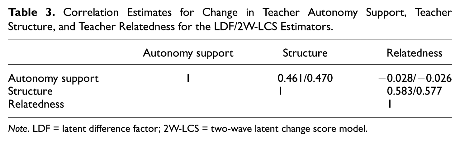
Note. LDF = latent difference factor; 2W-LCS = two-wave latent change score model.

Discussion

The purpose of this study was to compare the performance of two methods, the LDF and 2W-LCS, for modeling correlation in the change of latent variables between two points in time. In many situations, researchers collect data at two occasions and need to know whether changes in latent variables between the times are correlated with one another. As an example, we examined the correlation among changes in teacher practices in the classroom using both the LDF and 2W-LCS. Although it is certainly preferable when possible for researchers to gather data at more than two time points, it is not always feasible to do so. For example, some large-scale testing programs such as that conducted by the Northwest Evaluation Association are carried out in a biannual fashion. Thus, researchers using data generated from such programs will only have data at these two time points, with which to work. In addition, data collection costs in terms of time, personnel, and resources may be prohibitive to the extent that measurements can only be made at two points in time. With just two time points, it is not possible for researchers to use an approach such as GCM to characterize the change over time, because it requires at least three time points in order to fit a model. In such instances, the two approaches that were the focus of the current study may prove to be particularly useful.

Overall, results of the simulation study comparing LDF and 2W-LCS revealed that they performed similarly across most conditions. Across most conditions, both methods had no problems converging. However, when the factor structure was relatively weak (low loadings, few indicators, low interfactor correlation) and the sample size was relatively small, convergence rates were not 100%. Given its relatively greater complexity, we hypothesized that the 2W-LCS would have somewhat greater difficulty in attaining convergence for small sample sizes than would LDF. However, this did not turn out to be the case. In the few instances where convergence was an issue, it was more of a problem for LDF than for 2W-LCS, but even then the convergence rates were always in excess of 95%. For each technique, performance in the form of MSE, estimate bias, and estimate standard error was better with larger samples, more factor indicators, and stronger relationships between the indicators and the factors. In addition, the magnitude of the underlying factor did not have any bearing on the performance of these methods. In concordance with what was posited above, estimation bias for the two methods was low, peaking at approximately 0.055, but generally falling below 0.03 in most situations. Finally, both approaches yielded overestimates of the correlation between changes in the factors, across both methods used here.

Though performance of LDF and 2W-LCS was similar, there were some differences between the two. For the most part, 2W-LCS yielded somewhat more efficient estimates than did LDF, particularly when 10 or 15 indicators were present, and when the sample size was 500 or less. On the other hand, estimation bias for LDF was lower than that of 2W-LCS for the smallest sample size and for 10 or 15 indicators. Relatively weak factor loadings (0.5) were associated with greater bias for LDF. Indeed, there were some problems in estimation for both methods associated with weak loadings and a small number of indicators (3 or 5) per factor, as was made clear by the MSE. However, these problems were slightly more pronounced for LDF as compared to 2W-LCS. Across most conditions, the standard errors for 2W-LCS were lower than was the case for LDF, which was partly in keeping with what was hypothesized above. We anticipated that 2W-LCS would yield lower standard errors for larger samples and more indicators per factor, but did not expect to see this with smaller sample sizes, in particular. However, it appears that in fact 2W-LCS exhibited fewer problems with small samples than we anticipated would be the case.

Implications for Practice

When considering the implications of these results for practice, the researcher should take several considerations into account. First, when the sample size exceeds 500, and/or the factor loadings are 1 or larger, it would appear that the two methods will yield very similar results to one another. When factors have relatively few indicators (5 or less), and the indicators have a relatively weak association with the factors (0.5), then 2W-LCS may be a preferable alternative to LDF. On the other hand, when factors have 10 or more indicators each, LDF will yield somewhat less biased results than will 2W-LCS, though its standard errors will be slightly larger. Nonetheless, if the main desire in such cases is to estimate the correlation in factor change scores as accurately as possible, LDF may be preferable to 2W-LCS when 10 or more indicators per factor are present. Finally, one additional advantage of 2W-LCS that has been cited by Henk and Castro-Schilo (2016) is that it allows for the estimation of factor mean change scores, as well as the correlation between these changes. These means can also be estimated in the process of fitting the LDF models, as each individual factor model must be fit prior to fitting the LDF itself. However, it is the case that the 2W-LCS model is fit in a single step, thereby allowing for a relatively easy estimation of the latent variables’ means. Finally, though perhaps not a large consideration, it is true that the LDF model is simpler than the 2W-LCS, so that in particular with complex models involving a large number of factors and indicators, the LDF would be potentially easier to program.

Limitations and Directions for Future Research

It must be acknowledged, as was done above, that examining pairwise differences, as is the case here, is not an ideal situation. Certainly, when possible researchers should make a point to collect data at more than two time points when conducting longitudinal research. By doing so, they are better able to capture the true nature of change in the latent traits of interest in the form of more complex and potentially nonlinear models. In addition, by having more than two time points with which to work, the estimated relationships among change in latent variable scores will be more stable. With respect to the current study, future work in this area should expand the set of simulation conditions from those examined here, including more extreme correlations between latent trait changes, in order to account for how well LDF and 2W-LCS perform at the boundary conditions. In addition, future research should also extend the types of indicators from normally distributed continuous to categorical variables. Such variables are very common in latent variable modeling, particularly in the form of Likert-type questionnaire items, and thus should be examined in the context of latent change scores. Future research could also examine extensions of the LDF and 2W-LCS models to accommodate covariates in the form of MIMIC models, or structural models in which more complex relationships in change over time scores were modeled.

Conclusions

Though certainly not ideal, many researchers in practice are faced with the situation in which they need to examine relationships in change of latent variables over time and data are available at only two time points. In such cases, the LDF and 2W-LCS models examined here may be quite useful, given the results of the simulation study, coupled with prior work examining the 2W-LCS using empirical data. Both approaches yielded relatively low correlation estimate bias and standard errors, across a variety of sample sizes, number of indicators, and factor loading magnitude conditions. Recommendations for which to use when would be that when there are 10 or more indicators per factor, LDF will yield somewhat less biased estimates than will 2W-LCS. On the other hand, when there are fewer indicators per factor, 2W-LCS may be preferable to LDF, unless the sample size is 300 or less, in which case LDF will yield the least biased correlation estimates. Finally, though not a major issue, the computer code for fitting the LDF model is simpler than that for fitting the 2W-LCS. This is not a major advantage for fairly simple models, such as the ones described in the current study. However, for larger models with more indicators and more factors, the relative simplicity of the LDF could be an advantage in practice.

Footnotes

Declaration of Conflicting Interests

The author(s) declared no potential conflicts of interest with respect to the research, authorship, and/or publication of this article.

Funding

The author(s) received no financial support for the research, authorship, and/or publication of this article.

References

Belmont

Skinner

Wellborn

Connell

(1992). Teacher as Social Context (TASC). Student report measures of teacher provision of involvement, structure, and autonomy support (Technical Report). Rochester, NY: University of Rochester.

Budiman

Halim

Mohd Meerah

Osman

(2014). The effects of cognitive conflict management on cognitive development and science achievement. International Journal of Science and Mathematics Education, 12, 1169-1195.

Cohen

(1988). Statistical Power Analysis for the Behavioral Sciences. New York, NY: Routledge.

Henk

C. M.

Castro-Schilo

(2016). Preliminary detection of relations among dynamic processes with two-occasion data. Structural Equation Modeling, 23, 180-193.

Kline

R. B.

(2016). Principles and practice of structural equation modeling. New York, NY: Guilford Press.

Little

T. D.

Preacher

K. J.

Selig

J. P.

Card

N. A.

(2007). New developments in latent variable panel analyses of longitudinal data. International Journal of Behavioral Development, 31, 357-365.

McArdle

J. J.

Nesselroade

J. R.

(1994). Using multivariate data to structure developmental change. In Cohen

S. H.

Reese

H. W.

(Eds.), Life span developmental psychology: Methodological innovations (pp. 223-267). Hillsdale, NJ: Erlbaum.

Mohammed

Majid

Abdullah

(2016). The differential effect of attentional condition on subsequent vocabulary development. English Language Teaching, 9(1), 88-100.

Muthén

L. K.

Muthén

B. O.

(2015). Mplus user’s guide (7th ed.). Los Angeles, CA: Muthén & Muthén.

10.

Purpura

Logan

(2015). The nonlinear relations of the approximate number system and mathematical language to early mathematics development. Developmental Psychology, 51, 1717-1724.

11.

R Development Core Team. (2015). R: A language and environment for statistical computing. Vienna, Austria: R Foundation for Statistical Computing.

12.

Ralston

Bays

(2015). Critical thinking development in undergraduate engineering students from freshman through senior year: A 3-cohort longitudinal study. American Journal of Engineering Education, 6(2), 85-98.

13.

Ryan

R. M.

Deci

E. L.

(2000). Self-determination theory and the facilitation of intrinsic motivation, social development, and well-being. The American Psychologist, 55, 68-78.

14.

Selig

J. P.

Preacher

K. J.

(2009). Mediation models for longitudinal data in developmental research. Research in Human Development, 6, 144-164.