
Abstract
When item scores are ordered categorical, categorical omega can be computed based on the parameter estimates from a factor analysis model using frequentist estimators such as diagonally weighted least squares. When the sample size is relatively small and thresholds are different across items, using diagonally weighted least squares can yield a substantially biased estimate of categorical omega. In this study, we applied Bayesian estimation methods for computing categorical omega. The simulation study investigated the performance of categorical omega under a variety of conditions through manipulating the scale length, number of response categories, distributions of the categorical variable, heterogeneities of thresholds across items, and prior distributions for model parameters. The Bayes estimator appears to be a promising method for estimating categorical omega. Mplus and SAS codes for computing categorical omega were provided.
A scale is said to be reliable if scale scores can be replicated for individuals under similar measurement conditions (Crocker & Algina, 1986). Consider an individual randomly selected from a population. Classical true score theory (CTT) states that the individual’s observed score on a scale, Xi, is the sum of the true score, Ti, and the error score, Ei (Lord & Novick, 1968):

where Ti is defined as the expectation of the observed score over repeated measurements, Ti = E(Xi). In addition, E(Ei) = 0 and the correlation between Ti and Ei is zero. In educational and psychological testing, the variability of scale scores across individuals is often of interest. Assuming that Equation (1) holds true for every individual randomly selected from a population, the CTT model is expressed for the population as (see Lord & Novick, 1968)

where the subscript i is removed. Then reliability is defined as the correlation between the scale scores (X) and the scores obtained from the repeated administration of the same scale or the parallel form (X′), and is symbolized as ρXX′ (Crocker & Algina, 1986; Lord & Novick, 1968):

where σXX′, σX, and σX′ denote the covariance between scale scores and the scores from the parallel form, the standard deviation of scale scores, and the standard deviation of scale scores from the parallel form, respectively. In the current article, this definition of reliability is referred to as Definition 1. Under the assumptions of CTT, Equation (3) is mathematically equivalent to the squared correlation between scale scores and true scores (
Coefficient omega (Heise & Bohrnstedt, 1970; McDonald, 1999) has become a popular method for assessing the reliability of scale scores. Coefficient omega is based on factor analysis. Within the factor analysis framework, the observed score x for an item is expressed as (e.g., Bollen, 1989)

where v is the intercept,

Then, coefficient omega for the scale score that is the sum of J item scores is defined as (Bentler, 2009; Heise & Bohrnstedt, 1970; McDonald, 1999):

where
Coefficient Omega for Ordered Categorical Items
In educational and psychological research, data collected from participants are often represented by ordered categories (e.g., 4-point Likert-type scales). An ordered categorical variable is an ordinal version of a continuous, normally distributed latent response variable (e.g., Bollen, 1989). This view has been referred to as the underlying normal variable assumption (Raykov & Marcoulides, 2015) or the latent response variable formulation (Muthén & Muthén, 1998-2015). This assumption has been widely adopted in structural equation modeling for ordered categorical variables. Under this assumption, the common factor model and the relationship between the underlying continuous variable and the ordered categorical variable are expressed as (Bollen, 1989; Muthén, 1978)

with

where x* is the underlying continuous variable;
Green and Yang (2009) adopted Definition 1 to derive a reliability coefficient for the scale scores (i.e., the scores summed across J ordered categorical items). This derived reliability coefficient was labeled as
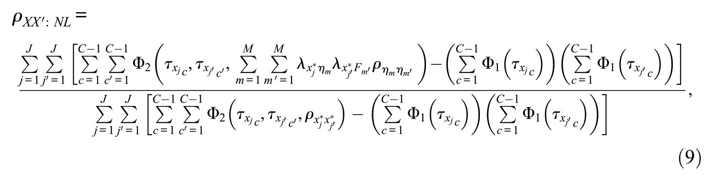
where
To demonstrate the problem of computing a reliability coefficient for ordered categorical items using Definition 2 and Definition 3, we created a hypothetical scale based on Equation (7) and Equation (8). The scale consisted of four binary items measuring a common factor. The loadings were .8 and the residual variances were .36 for all items. The thresholds were 1, .5, −1, and −.5 for Item 1 to Item 4, respectively, representing a realistic scenario in applied research in which the probabilities of endorsing categories tend to be different across items. The population Pearson covariance matrix and tetrachoric correlation matrix among these four binary variables were
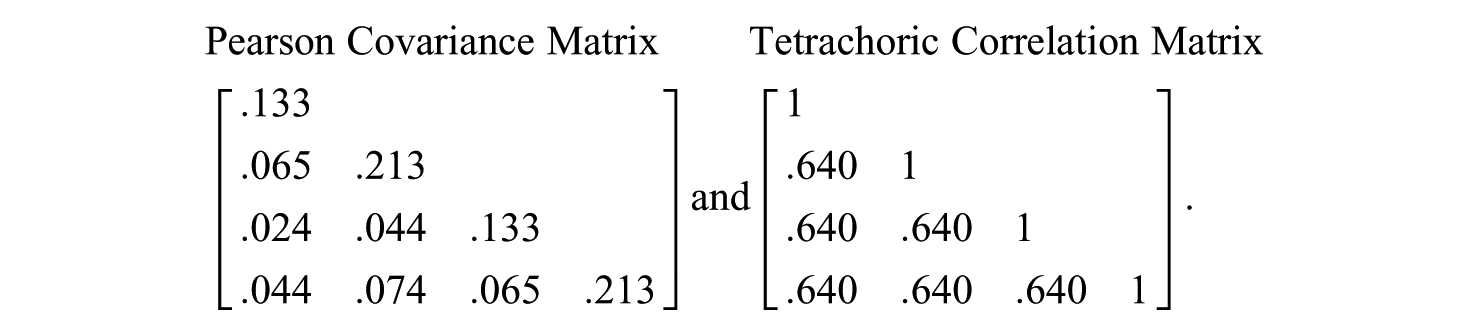
To obtain the reliability coefficient based on Definition 2 and Definition 3, we fit the Pearson covariance matrix to a linear one-factor model using maximum likelihood estimation in EQS 6.3 (Bentler, 1985-2017; EQS command files are available on request). The scale’s true-score and observed-score variances were estimated by creating auxiliary variables following the procedure outlined in Raykov and Shrout (2002). The coefficient omega estimates based on Definition 2 and Definition 3 were both .645. We then applied Equation (9) and obtained a categorical omega of .692. Next, we generated continuous item data for a sample with 1,000,000 observations for a scale and a parallel form based on the model parameters specified earlier. We dichotomized the continuous data using the thresholds specified above, computed the sum across binary items for the scale and its parallel form, respectively. We obtained a correlation of .692 between the scale scores and scores from its parallel form (Definition 3). This example illustrates that Equation (9) can provide an accurate estimate of reliability for scale scores. However, Definition 2 and Definition 3 yielded underestimates of reliability when the thresholds were different across items. In addition, fitting the linear model to the covariance matrix resulted in inadequate model–data fit with comparative fit index = .913 and root mean square error of approximation = .147. For more details regarding the comparison between omega and categorical omega, see Green and Yang (2009) and Yang and Green (2015).
The focus of the current study is to employ Bayesian estimation to compute categorical omega and to evaluate the performance of this estimation approach under a variety of manipulated conditions using computer generated data. This study is motivated by the findings from previous studies. On one hand, when a frequentist estimator (i.e., WLSMV) was used, categorical omega tended to be biased for short scales with binary items unless the sample size was larger than 500 (Yang & Green, 2015). On the other hand, several recent studies have provided promising evidence for the application of Bayesian structural equation modeling (BSEM) to categorical data under small sample size conditions (e.g., Holtmann, Koch, Lochner, & Eid, 2016; Liang & Yang, 2014; Nguyen, Webb-Vargas, Koning, & Stuart, 2016). Below we summarize the difficulties encountered in categorical omega estimation using frequentist estimators, and then introduce Bayesian estimation to compute categorical omega.
Difficulties Encountered in Categorical Omega Estimation Using Frequentist Estimators
To estimate categorical omega from sample data, a factor analysis model is fit to the data with an estimator that is appropriate for ordinal variables. The most commonly applied estimator is diagonally weighted least squares (DWLS). It is implemented as the mean- and variance-adjusted weighted least squares (WLSMV) and the mean-adjusted weighted least squares (WLSM) in Mplus 7 (Muthén & Muthén, 1998-2015) and the lavaan package in R (Rosseel, 2012). WLSMV appears to be more popular than WLSM in structural equation modeling (SEM) applications. DWLS fits polychoric correlations (or tetrachoric correlations for binary variables) and thresholds to a hypothesized model. In both Mplus and the lavaan package, thresholds and polychoric correlations are estimated by default using a 2-stage maximum likelihood (ML) estimation procedure (Olsson, 1979). In the 2-stage procedure, thresholds for each variable are first estimated based on the cumulative marginal proportions in the contingency table. In the second stage, the thresholds are treated as fixed and the polychoric correlations between all possible pairs of the underlying continuous variables are estimated. When the population threshold values are large (e.g., >2 assuming x* ~ N(0, 1)), the marginal probabilities for some categories may be very small. The estimated thresholds based on the observed marginal probabilities may thus be inaccurate in finite samples. Also, when the distributions of two ordinal variables are highly skewed and/or skewed in opposite directions, some cells can have very small probabilities and thus contain only a few observations. In these circumstances, the estimated polychoric correlations tend to be inaccurate (e.g., Olsson, 1979; Savalei, 2011). Previous simulation studies have shown that model results based on polychoric correlations can be inaccurate for small samples, two to four categories, and large threshold values (DiStefano & Morgan, 2014; Garrido, Abad, & Ponsoda, 2016; Rhemtulla, Brosseau-Liard, & Savalei, 2012; Savalei & Rhemtulla, 2013; Yang & Xia, 2015; Yang-Wallentin, Jöreskog, & Luo, 2010).
Because categorical omega is a function of model parameters that are estimated by fitting a model to polychoric correlations and thresholds, we suspect that the bias arising from the 2-stage ML estimation of polychoric correlations and thresholds could lead to a biased estimate of categorical omega for relatively small sample sizes and/or with highly skewed categorical distributions. In a recent simulation study, Yang and Green (2015) evaluated the performance of categorical omega under a variety of conditions. They found that when the categorical distributions were highly skewed and varied across items, categorical omega can be substantially biased (e.g., mean sample estimate = .645 vs. population categorical omega = .750). They suggested that a sample size larger than 500 may be needed to accurately estimate categorical omega for a scale with eight binary items, which is unrealistic for many small-scale studies. We argued that alternative methods should be chosen for estimating categorical omega with relatively small sample sizes (≤500).
Categorical Omega Using Bayesian Structural Equation Modeling
Bayesian estimation methods have recently received increasing attention in the field of SEM. Instead of being treated as fixed in the frequentist approaches, model parameters in BSEM are random variables following certain distributions. Applying Bayes’ theorem to a factor analysis model with categorical items (Asparouhov & Muthén, 2010):
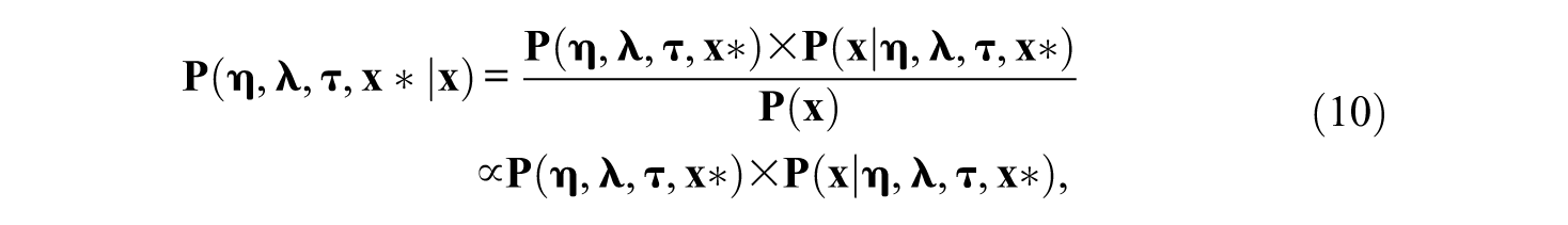
which states that the posterior distribution for model parameters
Commonly, posterior distributions are empirically approximated using Markov chain Monte Carlo (MCMC) algorithms (Gilks, Richardson, & Spiegelhalter, 1996). The Gibbs sampler (Geman & Geman, 1984) is one of the most popular MCMC algorithms for approximating the posterior distributions and is implemented in Mplus by default. In a Bayesian factor-analysis model with categorical items, parameters are divided into four groups and are updated in sequence: (1) update
As in SEM analyses, evaluation of model–data fit is essential in BSEM. The parameter estimates (and consequently categorical omega) are likely to be biased if the model fails to demonstrate an adequate fit to the data. In BSEM, model–data fit can be evaluated through the posterior predictive checking (PPC) procedure, which does not depend on asymptotic theory (e.g., Asparouhov & Muthén, 2010). A predictive posterior p-value (PPP) compares the discrepancy function from the observed data to that from the data drawn from the posterior distributions at each iteration. If the model is consistent with the data, the PPP is around .50. Asparouhov and Muthén (2010) suggested that a PPP less than .05 or .01 indicates poor model–data fit.
Several recent studies have provided promising evidence for the application of BSEM to categorical data. For example, Liang and Yang (2014) found that Bayesian factor analysis resulted in more accurate parameter estimation than WLSMV when sample sizes were small or when categorical distributions were greatly asymmetric. Nguyen et al. (2016) compared ML, WLSMV, and BSEM in causal mediation analysis with a binary outcome and multiple mediators. Their results showed that BSEM outperformed ML and WLSMV when the mediators were ordered categorical. Based on the findings from these previous studies, we expected that the substantial bias of thresholds, polychoric correlations, and consequently categorical omega found when using frequentist methods may be alleviated by employing Bayesian factor analysis. This should be particularly true when the sample size is relatively small and the categorical items present varying degrees of asymmetricity. In addition, it is known that the posterior distributions of model parameters are dependent on the selection of prior distributions. Many priors are available, but some priors (e.g., those implemented by default in Mplus) may be used more often than others in applications. How does categorical omega perform when these priors are specified? The current simulation study addresses this research question.
Selection of Priors in Bayesian Factor Analysis for Categorical Omega Estimation
To estimate categorical omega using BSEM, a prior distribution should be selected for each model parameter including factor loadings, thresholds, and factor covariances. Priors can range from noninformative to informative, representing little to substantial amounts of prior knowledge about the parameters. One important topic in applied Bayesian analysis is the sensitivity of model results to the selection of prior distributions. When the sample size involved in the analysis is small, priors can have a large impact on the formulation of posterior distributions (Lee, 2007; Muthén & Asparouhov, 2012). For example, within the multilevel SEM framework, Holtmann, et al. (2016) found that Bayesian estimation performed as well as or outperformed WLSMV for categorical variables with small sample sizes when the selected priors were informative. In empirical studies, accurate information on parameters is often not available; instead, noninformative or weakly informative prior distributions are frequently selected (e.g., N(0, 1) for factor loadings). The default priors implemented in Mplus are mostly noninformative (e.g., N(0, 5) for factor loadings). We considered the default priors and several selected weakly informative priors in the current simulation study (more details in the Method section).
In Mplus 7 the priors are specified for unstandardized parameters that are based on the theta parameterization. However, the metric of loadings and thresholds for computing categorical omega is consistent with the delta parameterization (see Equation 9). When the variance of each factor is fixed at one, the conversion of thresholds and factor loadings between the two parameterizations is (Finney & DiStefano, 2013)

where the subscripts theta and delta indicate the parameters based on the theta parameterization and delta parameterization, and λ,
In the current simulation study, we applied priors with means of population threshold values and factor loadings that are consistent with both delta and theta parameterizations for two reasons: (1) applied researchers have some knowledge about threshold and loading parameters and may want to select (weakly) informative priors and (2) applied researchers may not realize that the prior distributions in Mplus are applied to the unstandardized parameters consistent with the theta parameterization and may mistakenly apply priors that are consistent with the delta parameterization.
We conducted a simulation study by manipulating various design factors to evaluate the performance of categorical omega using Bayesian estimation methods. Specifically, we aimed to answer the following two questions. First, is the categorical omega obtained using Bayesian estimation relatively accurate? For this question, we focused on conditions with relatively small sample sizes (≤500) and large differences in thresholds across items, because categorical omega was shown to be greatly biased under these conditions when using WLSMV (Yang & Green, 2015). Second, how sensitive is categorical omega to the selected prior specifications? Below we describe the details of the simulation study.
Method
Design Factors for Data Generation
Factor Structure
We considered two factor structures. One was a one-factor model in which all items loaded on one common factor with no correlated residuals. The second was a bifactor model in which all items loaded on a general factor and subgroups of items loaded on two or four group factors. The correlations among factors were all zero in the bifactor model. We included the bifactor structure because many tests are designed to measure multidimensional constructs and the bifactor model has received much attention in the literature (e.g., Reise, Scheines, Widaman, & Haviland, 2013).
Scale Length
Two scales were considered. One contained eight items and the other contained 16 items. Because factor loadings tend to be unequal across items in practice, we specified the factor loading vector for the one-factor model as

for the 8-item scale, and

for the 16-item scale. For the bifactor model, the factor loading vector was defined as

for the 8-item scale with two group factors, and
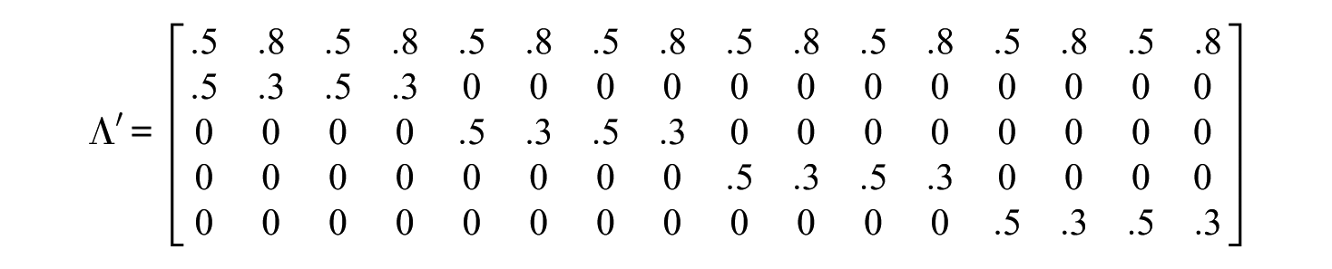
for the 16-item scale with four group factors.
The models described above were used to generate continuous item data according to Equation (7). For both models, the intercept v for each item was zero and the factor scores followed N(0, 1). The residual covariance matrix was a diagonal matrix with its diagonal elements being
Thresholds
After the continuous item data were generated, thresholds were applied to create ordered categorical item data. The number of categories for each item was either two or four. For the 2-category items, five thresholds were chosen: {−1.5}, {−.5}, {0}, {.5}, and {1.5}, resulting in response probabilities of {7%, 93%}, {31%, 69%}, {50%, 50%}, {69%, 31%}, and {93%, 7%} in the population, respectively. For the 4-category items, five sets of thresholds were chosen: {−1.5, −1, −.5}, {−1, −.5, 0}, {−.5, 0, .5}, {0, .5, 1}, and {.5, 1, 1.5}, resulting in response probabilities of {6.7%, 9.2%, 15.0%, 69.1%}, {15.9%, 15.0%, 19.1%, 50.0%}, {30.9%, 19.1%, 19.1%, 30.9%}, {50.0%, 19.1%, 15.0%, 15.9%}, and {69.1%, 15.0%, 9.2%, 6.7%} in the population, respectively. These thresholds yielded different categorical distributions ranging from negatively skewed to positively skewed. These sets of thresholds were next used to create four scales with varying degrees of dissimilarities in thresholds, which were labeled as homogenous scale, mildly heterogeneous scale, moderately heterogeneous scale, and highly heterogeneous scale, respectively. The assignment of thresholds to each item to form these scales is shown in Table 1. For example, for scales with eight binary items, the homogenous scale had a threshold of {0} for all items. For the moderately heterogeneous scale, the first four items had a threshold of {−.5} and the last four items had a threshold of {.5}. For the highly heterogeneous scale, the first four items had a threshold of {−1.5} and the last four items had a threshold of {1.5}.
Thresholds Used to Create Ordered Categorical Item Data.
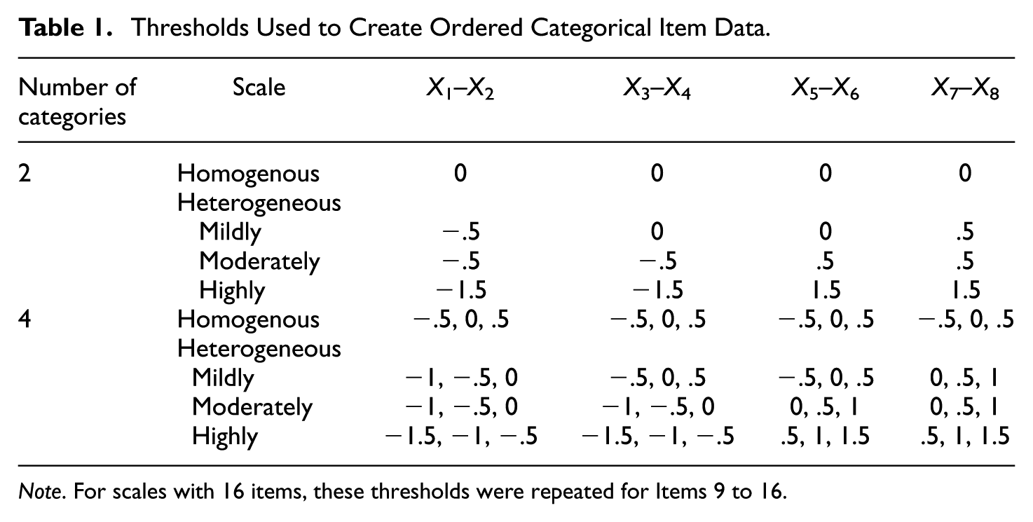
Note. For scales with 16 items, these thresholds were repeated for Items 9 to 16.
Sample Size
The sample size was either 50, 100, 200, or 500. A sample size of 50 is considered very small for a factor analysis with 8 or 16 items. A sample size of 500 is the recommended minimum sample size for adequate estimate of categorical omega for eight-item scales using WLSMV (Yang & Green, 2015).
The total number of conditions for data generation was 2 (factor structure) × 2 (scale length) × 2 (number of categories per item) × 4 (scale heterogeneity) × 4 (sample size) = 128. For each condition, 2,000 data sets were generated.
Analysis Models and Prior Distributions
Each data set was fit to a model that was consistent with the data generation model, specifically, either the one-factor model or the bifactor model. All models were analyzed in Mplus 7. The factor variance was fixed at one. The model parameters included loadings and thresholds.
For each model parameter, a prior distribution should be selected. The priors for both thresholds and loadings followed normal distributions. For loadings, the normal prior is the conjugate prior such that the posterior distribution and the prior distribution are in the same distribution family. As justified in the previous section, we selected four priors for loadings: N(
λ ~ N(λ
theta
, 1), τ ~ N(
λ ~ N(0, 1), τ ~ N(0, 1)
λ ~ N(0, 1), τ ~ N(0, 5)
λ ~ N(λ delta , 5), τ ~ N(0, 5)
λ ~ N(0, 5), τ ~ N(0, 5)
The prior specifications resulted in five analysis models for each data set. The total number of combinations for data analyses was 5 (sets of priors) × 128 (data generation conditions) = 640. For each analysis model, two MCMC chains were used. The first half of each chain was considered as the burn-in period. The remaining iterations were used to form the posterior distributions of the parameters and for convergence evaluations. Model convergence was determined by the Gelman-Rubin convergence criterion with the default value of .05 in Mplus. The default maximum number of iterations in Mplus is 50,000. We conducted some preliminary analyses and found that up to 25% of data sets did not satisfy the convergence criterion with the 50,000 iterations for the bifactor models. Based on the results from the preliminary analyses, we increased the maximum number of iterations to 300,000. With this maximum number of iterations, all analyses met the convergence criterion and produced proper solutions.
Results
From each analysis, we obtained the medians of the posterior distributions for model parameters (i.e., factor loadings and thresholds) and substituted them into Equation (9) to compute the sample categorical omega. We then computed the mean and standard deviation of sample categorical omegas for each condition. For model–data fit evaluation, we computed the mean PPPs across 2,000 replications and the percentage of replications with PPP < .05 for each condition. The results are shown in the eight supplementary tables (available in the online version of the article) and are summarized below.
Categorical Omega
Figure 1 and Figure 2 display the mean categorical omegas for the conditions with one-factor models and bifactor models, respectively. The horizontal dotted line in each graph represents the population categorical omega, which was computed by substituting the population values of factor loadings and thresholds into Equation (9). The population categorical omegas ranged from .554 to .931, covering a wide range of reliability from unsatisfactory to excellent. The means for the conditions with mildly heterogeneous scales are not shown in the figures because they were very close to those from the conditions with homogenous scales. Because the results from the conditions with homogenous, mildly heterogeneous, and moderately heterogeneous thresholds across items were very different from those with highly heterogeneous thresholds across items, we summarized these two groups of conditions separately.
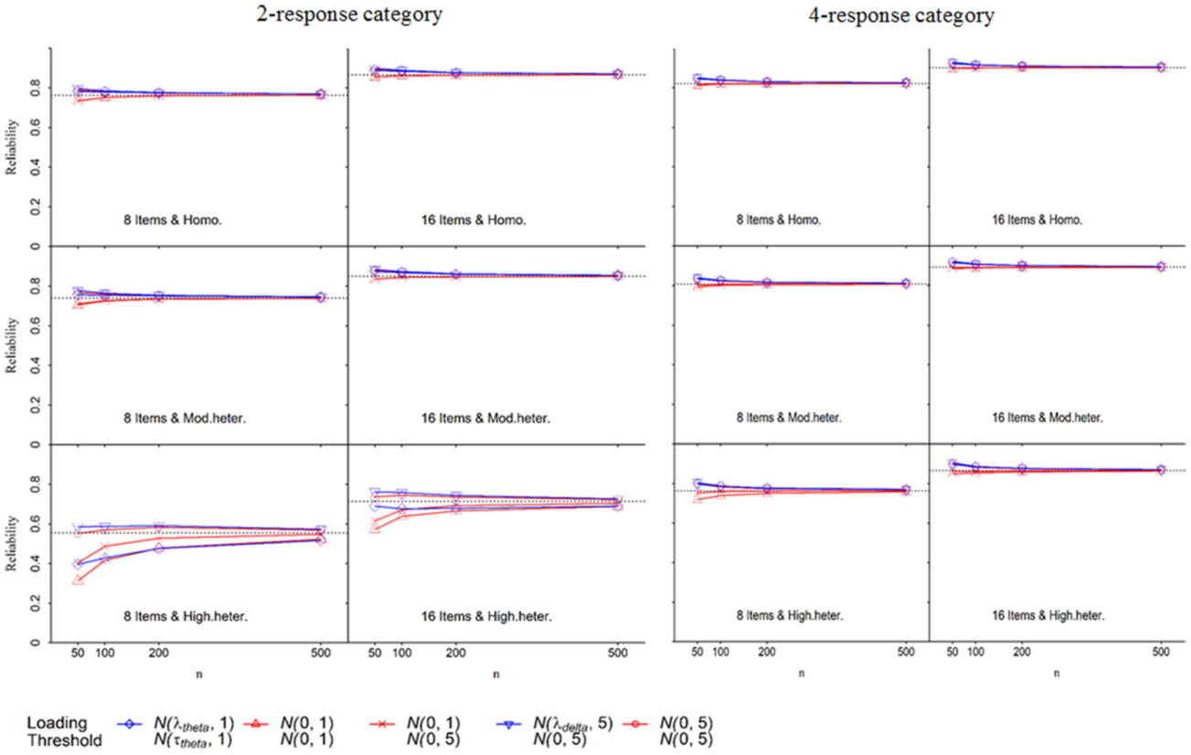
Means of sample categorical omegas from one-factor models.

Means of sample categorical omegas from bifactor models.
Conditions With Homogenous, Mildly Heterogeneous, and Moderately Heterogeneous Thresholds Across Items
In general, the sample categorical omega tended to slightly underestimate the population categorical omega when the prior λ ~ N(0, 1) was used, but tended to overestimate the population categorical omega when other priors were used. The prior λ ~ N(λ
delta
, 5) resulted in the greatest positive bias of categorical omega and the bias was most prominent when the sample size was 50, the number of items was eight, and the number of response categories was two. However, even under these worst conditions, the absolute bias was not greater than .04 (i.e.,
The standard deviations of the categorical omegas are not shown in the figures. In summary, the standard deviations decreased as the sample size increased. The priors λ ~ N(λ
theta
, 1) and τ ~ N(
Conditions With Highly Heterogeneous Thresholds Across Items
When the sample size was 50, categorical omega was substantially biased (with
The standard deviation of the sample categorical omegas for each condition is not shown in the figures. Among the selected priors, the prior λ ~ N(0, 1) resulted in the largest standard deviation. As the sample size increased, standard deviations decreased and became comparable across the priors.
Evaluation of Model–Data Fit Based on PPPs
We next summarize the results of model–data fit evaluations based on the PPPs. The mean PPP and the percentage of replications with PPP < .05 for each condition are available as Supplementary Tables 5 to 8 (available in the online version of the article). For the conditions with homogenous, mildly heterogeneous, or moderately heterogeneous thresholds across items, the mean PPPs were all around .50 with a range of .42 to .59. No more than one replication per condition yielded PPP < .05. These results indicated that the model–data fit was good.
Table 2 presents the mean PPPs and the percentages of replications with PPP < .05 for conditions with highly heterogeneous thresholds across items. PPPs varied across sample sizes and different priors. For conditions either with the sample size of 500 (not shown in Table 2) or with the following three sets of priors, the mean PPPs were all around .50: (a) λ ~ N(0, 1) and τ ~ N(0, 5), (b) λ ~ N(λ
delta
, 5) and τ ~ N(0, 5), and (c) λ ~ N(0, 5) and τ ~ N(0, 5). For these conditions, no more than two replications per condition resulted in PPP < .05. However, for conditions with sample sizes ≤200 and the other two sets of priors (i.e., λ ~ N(λ
theta
, 1) and τ ~ N(
Mean PPPs (% of Replications With PPP < .05) for Scales With Highly Heterogeneous Thresholds.
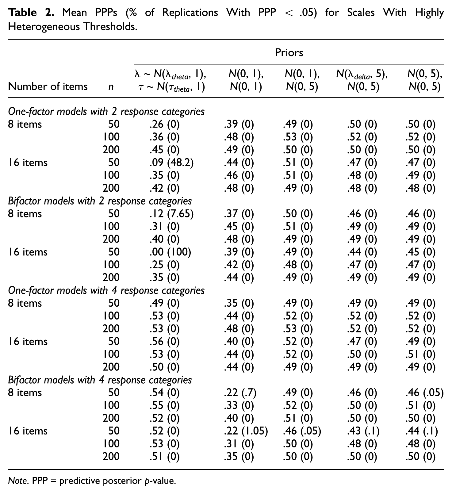
Note. PPP = predictive posterior p-value.
Summarization and Discussion
In this article, we discussed the problems of fitting a SEM model to polychoric correlations and thresholds using DWLS and computing categorical omega. When the sample size is relatively small and the thresholds are different across ordered categorical items, the estimated categorical omega can be substantially biased, particularly when the number of items is small (Yang & Green, 2015). Acquiring a large sample size may alleviate the problems but most often it is not pragmatic and in some cases may not be possible. We suggest applying Bayesian estimation methods to analyze the structural equation model and to compute categorical omega. The current simulation study examined whether Bayesian estimation methods could result in an accurate estimate of categorical omega under finite samples for scales with different length, number of response categories, distributions of the categorical variables, and heterogeneity of thresholds across items. We examined several priors for loadings and thresholds parameters ranging from noninformative to informative in this simulation study. Our simulation study showed that the Bayes estimator was in general a promising method for estimating categorical omega, although it did perform differently under different combinations of conditions. Below we offer suggestions to applied researchers when using a Bayes approach for estimating categorical omega.
The results from our simulation study suggested that mean categorical omegas were very close to population values when the thresholds across items were not highly heterogeneous, regardless of the sample size (as small as 50) and the selection of priors. For these conditions, the mean PPPs were all around .50, indicating good model–data fit. Given an empirical data set, the observed ordered categorical distribution for each item can be examined. If a researcher finds that the distributions of categorical variables are relatively similar (e.g., not a mixture of positively skewed and negatively skewed distributions), the choice of prior distributions is less of a concern. In such cases, all the selected priors gave very accurate estimates of categorical omega even when the sample size was as small as 50. In addition, the most informative pair of priors (i.e., λ ~ N(λ
theta
, 1) and τ ~ N(
The results from our simulation study also suggested that when thresholds were highly heterogeneous across items, the sample categorical omega tended to be substantially biased for scales with fewer items (i.e., eight), fewer response categories, and smaller sample sizes (<100) when the weakly informative prior (i.e., N(0, 1)) was applied to the factor loadings. For several of these conditions, the mean PPPs were much below the expectation of .50 (down to .00) and a large portion of the replications (up to 100%) yielded PPP<.05, indicating model–data misfit. The agreement between the bias of categorical omega and the model–data misfit is opportune because it should prevent applied researchers from adopting a poor fitting model and interpreting the resulting categorical omega. However, for the majority of these conditions, low PPP values (i.e., <.05) did not correspond to biased estimation of categorical omega. Evaluating model–data fit based on PPP may lead to model overspecification and further complicate the estimation of categorical omega. In addition, the prior λ ~ N(0, 1) yielded the greatest standard deviations of categorical omegas, while the standard deviations were comparable when other priors were used. Therefore, applied researchers may want to avoid using this prior for factor loadings when the thresholds are highly heterogeneous across items, the scale is short, and the sample is small.
Although a large number of conditions were considered in the simulation design, the current study shares similar limitations in terms of generalization of findings with many other simulation studies. In addition, all the analysis models in the study were correctly specified. Further studies are needed to examine the estimation of categorical omega under misspecified models, as well as the role of other fit indexes (e.g., Bayes factor, difference in AIC, and difference in DIC) in detecting correctly specified models.
Footnotes
Appendix
Acknowledgements
The authors would like to thank Betsy J. Becker and two anonymous reviewers for providing a careful review and constructive comments on earlier versions of the article.
Declaration of Conflicting Interests
The author(s) declared no potential conflicts of interest with respect to the research, authorship, and/or publication of this article.
Funding
The author(s) received no financial support for the research, authorship, and/or publication of this article.
Supplemental Material
Supplemental material is available for this article online.
References
Supplementary Material
Please find the following supplemental material available below.
For Open Access articles published under a Creative Commons License, all supplemental material carries the same license as the article it is associated with.
For non-Open Access articles published, all supplemental material carries a non-exclusive license, and permission requests for re-use of supplemental material or any part of supplemental material shall be sent directly to the copyright owner as specified in the copyright notice associated with the article.