Incorporating the Q-Matrix Into Multidimensional Item Response Theory Models

Abstract

Multidimensional item response theory (MIRT) models use data from individual item responses to estimate multiple latent traits of interest, making them useful in educational and psychological measurement, among other areas. When MIRT models are applied in practice, it is not uncommon to see that some items are designed to measure all latent traits while other items may only measure one or two traits. In order to facilitate a clear expression of which items measure which traits and formulate such relationships as a math function in MIRT models, we applied the concept of the Q-matrix commonly used in diagnostic classification models to MIRT models. In this study, we introduced how to incorporate a Q-matrix into an existing MIRT model, and demonstrated benefits of the proposed hybrid model through two simulation studies and an applied study. In addition, we showed the relative ease in modeling educational and psychological data through a Bayesian approach via the NUTS algorithm.

Keywords

Bayesian estimation diagnostic classification models Q-matrix multidimensional item response theory

Introduction

In social science research, assessments are developed to measure individuals’ latent traits. To analyze responses from assessment data, item response theory (IRT) models have evolved as a mainstream class of psychometric models since the 1970s (Lord & Novick, 1968).

Many current assessments developed under the IRT framework are unidimensional because multidimensional assessments require longer test lengths and larger examinee sample sizes. For example, an assessment can be designed to measure students’ math ability in education or self-esteem in the area of psychology as a unidimensional trait. Although unidimensional IRT models are commonly used, the assumption of trait unidimensionality is often difficult to meet in practice (e.g., Ackerman, 1994, 1996; Reckase, 1985). For example, correctly answering math items may also require reading skills to understand the item stems, and items measuring self-esteem may produce data that are confounded with relevant traits such as achievement or happiness. Ultimately, dimensionality is never a “black or white” question as no test data can be truly unidimensional (Liu, Huggins-Manley, & Bulut, 2018; Thissen, 2016).

When unidimensionality is violated or when a test is specifically designed to measure more than one trait, multidimensional IRT (MIRT) models can be used to model the complex interactions between an individual’s multiple abilities and items representing multiple constructs (Reckase, 2009). MIRT models are promising in education because teachers and students are often interested in obtaining scores on subscales, and they are also useful in psychology because personality assessments are often intended to measure more than one correlated trait.

Despite the advantages of MIRT models, their uses in practice are somewhat limited because the number of parameters in MIRT models is much larger than unidimensional IRT models (e.g., Drasgow & Parsons, 1983). As a result, MIRT models require long test lengths and large sample sizes for a reliable estimate of parameters and latent traits on multiple continua (e.g., Haberman & Sinharay, 2010; Maydeu-Olivares, 2001; Templin & Bradshaw, 2013).

More recently, a newer class of multidimensional models called diagnostic classification models (DCM; e.g., Rupp, Templin, & Henson, 2010) has become popular in psychometrics. Instead of locating examinees on multiple continua, DCMs classify examinees into groups based on their possession/nonpossession of certain traits. DCMs can achieve higher reliability than MIRT models for a given test length, all else being equal, mainly because of three unique features. First, the latent traits in DCMs are categorical so that the estimates of those traits have a smaller range, resulting in higher reliability (e.g., Templin & Bradshaw, 2013). Second, DCM reliability is commonly defined at the categorical level (Templin & Bradshaw, 2013), which results in higher coefficients as compared to those for continuous scores. We should note that categorical latent traits are less commonly seen than continuous latent traits in psychometrics. As discussed in Liu, Qian, Luo, and Woo (2017), the definition of reliability varies across IRT and DCM scoring approaches, but the overall concept of partitioning the total variance into true and error holds across different definitions. In DCMs, the use of categorical variables (e.g., 0 and 1) minimizes error, thus leading to higher reliability. Third, DCMs incorporate a prespecified relationship between items and latent traits (i.e., which items measure which traits). As a result, if an item is not designed to measure a particular trait, the associated parameters are not freely estimated. This relationship can be captured in an item by trait incidence matrix commonly known as a Q-matrix (Tatsuoka, 1983).

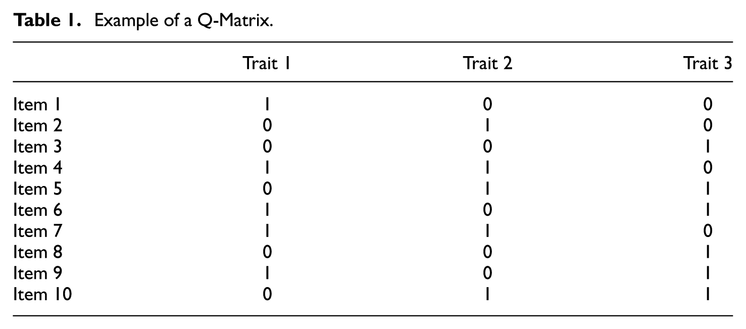
A Q-matrix is represented by a binary matrix that defines the relationship between items and latent traits (or skills in the cognitive context).

Table 1 is an example Q-matrix for dichotomous traits, although polytomous traits are also possible. In a dichotomous Q-matrix, an entry equals 1 if an item measures the trait and 0 otherwise. For example, Items 1 and 2 in Table 1 measure Traits 1 and 2, respectively. Using the Q-matrix in DCMs not only limits the number of parameters that need to be estimated and thus allows for smaller sample sizes and shorter test lengths, but also accurately reflects the item and test design considerations. Although the Q-matrix has such advantages, its use has largely been limited to research and application in DCMs.

Table 1.

Example of a Q-Matrix.

	Trait 1	Trait 2	Trait 3
Item 1	1	0	0
Item 2	0	1	0
Item 3	0	0	1
Item 4	1	1	0
Item 5	0	1	1
Item 6	1	0	1
Item 7	1	1	0
Item 8	0	0	1
Item 9	1	0	1
Item 10	0	1	1

The purpose of this study is to formulate the item–trait relationship in current MIRT models, incorporating information from experts or previous knowledge through a Q-matrix. Thus, a new formulation of MIRT models is defined in order to alleviate parameter estimation and provide a new interpretation of MIRT modeling.

We want to stress that researchers and practitioners have previously restricted the item–trait relationship when implementing MIRT models, and we are not in any way proposing new models. Instead, the study aims to explore the utility of the Q-matrix in MIRT models and propose a way to clearly express the item–trait relationship as a function in MIRT models. In this way, we add flexibility to the existing MIRT models and practitioners can tailor their models to a specific test through the Q-matrix specification.

To present and evaluate the idea of incorporating Q-matrices in MIRT models, we first formulate the multidimensional two-parameter logistic model with a Q-matrix (M2PL-Q model). Then, we report the results of two simulation studies. The first simulation study examined the parameter recovery of the M2PL-Q, and the second simulation study examined some impacts of using the correct Q-matrix as compared to using an item–trait fully crossed model and a bifactor model. Next, we report on an applied study that examined the performance of the M2PL-Q with real data. A discussion and conclusion are provided at the end.

The M2PL-Q Model

We consider a test designed to evaluate $D$ latent traits composed of $J$ binary items applied to $N$ individuals. Let the random variable $Y_{ij}$ be the answer of individual $i$ to item $j$ , such that

Y_{ij} | θ_{i}, ξ_{j} ~ Bernoulli (P_{ij}), i = 1, 2, \dots, n, j = 1, 2, \dots, J,

(1)

where $θ_{i} = (θ_{i 1}, θ_{i 2}, \dots, θ_{iD})$ is the parameter vector of individual $i$ such that $θ_{id}$ is the dth latent trait of individual $i$ ; $ξ_{j} = (a_{j 1}, a_{j 2}, \dots, a_{jD}, b_{j})$ is the vector of parameters associated with item $j$ such that $a_{jd}$ is a specific discrimination parameter of dimension $d$ and $b_{j}$ is the difficulty parameter of item $j$ ; and $P_{ij}$ is the probability of individual $i$ scoring 1 on item $j$ . According to the multidimensional two-parameter logistic (M2PL) model (Reckase, 2009), this probability can be written as

P_{ij} = P (Y_{ij} = 1 | θ_{i}, ξ_{j}) = \frac{\exp (η_{ij})}{1 + \exp (η_{ij})} = \frac{1}{1 + \exp (- η_{ij})},

(2)

where $η_{ij} = \sum_{d = 1}^{D} a_{jd} θ_{id} - b_{j}$ is called a latent linear predictor. As we can see, $η_{ij}$ is composed of a linear combination of $θ_{i 1}, θ_{i 2}, \dots, θ_{iD} .$ This linear combination can provide the same sum for various combinations of latent trait values through a compensation effect. Models with this characteristic are called compensatory models.

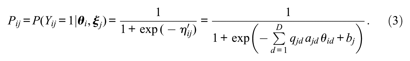
In order to present the multidimensional two-parameter logistic model with a Q-matrix (M2PL-Q model), we define the new latent linear predictor

η_{ij}' = \sum_{d = 1}^{D} q_{jd} a_{jd} θ_{id} - b_{j},

where $q_{jd}$ is the element of row $j$ and column $d$ of the Q-matrix such that $q_{jd} = 1$ if item $j$ evaluates dimension $d$ , and $q_{jd} = 0$ otherwise.

The probability of individual $i$ correctly answering item $j$ under the M2PL-Q model becomes

P_{ij} = P (Y_{ij} = 1 | θ_{i}, ξ_{j}) = \frac{1}{1 + \exp (- η_{ij}')} = \frac{1}{1 + \exp (- \sum_{d = 1}^{D} q_{jd} a_{jd} θ_{id} + b_{j})} .

(3)

Note that the M2PL-Q model is a generalization of other models. When we use the matrix full-Q, which is composed only of elements equal to 1, we obtain the M2PL model (described in Equation 2), which we call the M2PL-Q full model. In the same way, the bifactor 2PL model (Gibbons & Hedeker, 1992), which is characterized by considering a global latent trait and at least two other specific traits, can also be obtained from the M2PL-Q model. For this, it is enough to define a convenient Q-matrix, such that the first column, which corresponds to the global latent trait, is formed only by elements equal to 1, in order to allow all items to evaluate it; and the other columns, corresponding to the specific latent traits, are defined containing only one element equal to 1 per line, so that each item evaluates one, and only one, specific latent trait. We call a Q-matrix under these conditions a bifac-Q and the M2PL-Q model with the bifac-Q matrix is referred to as M2PL-Q bifac. In addition, when considering other particular cases where the Q-matrix is customized by experts (matrix custom-Q), we refer to a M2PL-Q custom model.

We present an example of the full-Q, bifac-Q, and custom-Q matrices for $J = 28$ and $D = 3$ in the appendix. When a Q-matrix is traditionally used in DCMs, one could specify one item that measures one or multiple latent traits. An item is known as simple-structured if it only measures one latent trait, and complex-structured if it measures multiple traits (Rupp & Templin, 2008b). Previous studies in DCMs have shown that tests with simple-structured items can produce higher classification accuracy because they may offer less confounded information about traits (e.g., Liu, Huggins-Manley, & Bradshaw, 2016; Madison & Bradshaw, 2015). Similarly, we expect that one would have more precise and less contaminated information when more simple-structured items are used in the M2PL-Q.

To obtain similar interpretations of the parameters from a one-dimensional IRT model, Reckase (2009) and Fragoso and Cúri (2013) suggest calculating the multidimensional parameters of each item. For the M2PL-Q, the discriminating power of the jth item is given by

MDIS C_{j} = \sqrt{\sum_{d = 1}^{D} q_{jd} a_{jd}^{2}} .

(4)

This measure encompasses only the discrimination parameters associated with the dimensions that each item measures and provides for each item an omnibus discrimination for all latent traits evaluated. Also, the multidimensional difficulty of the M2PL-Q, denoted by $MDIF F_{j}$ , referring to the jth item, is calculated on the scale of the latent trait as

MDIF F_{j} = \frac{b_{j}}{MDIS C_{j}} .

(5)

Bayesian Estimation

In this article, we propose using Bayesian estimation with Markov chain Monte Carlo (MCMC) algorithms to estimate the parameters of the M2PL-Q model. We define its likelihood and the prior distributions of its parameters. We also describe the No-U-Turn Sampler (NUTS) method, some model comparison criteria, and the posterior predictive distribution.

Likelihood

Let $y$ be the vector that contains all the responses of $N$ individuals to $J$ items, $θ$ be the vector that contains the parameters of the individuals, and $ξ$ be the vector that contains the parameters associated with all the items. Therefore, the likelihood for the M2PL-Q model can be written as

ℓ (y | θ, ξ) = Π_{i = 1}^{N} Π_{j = 1}^{J} P_{ij}^{w_{ij 1}} (1 - P_{ij})^{w_{ij 0}},

(6)

where $P_{ij}$ is defined by Equation 3, and $w_{ijk}$ is an indicator function such that $w_{ijk} = {\begin{matrix} 1, & if y_{ij} = k \\ 0, & if y_{ij} \neq k \end{matrix},$ for $k = 0, 1$ . The variable $w_{ijk}$ allows the use of missing data, since it considers in the likelihood only the observed data given by individuals.

Prior and Posterior Distributions

The specification of the prior distributions for the parameters of the model is an important procedure in the Bayesian analysis, since the posterior distributions of the parameters are influenced by both the sample and the prior distribution. This influence is due to the fact that the posterior distributions are defined as being proportional to the product of the likelihood described in Equation 6 and the prior distributions of the model parameters.

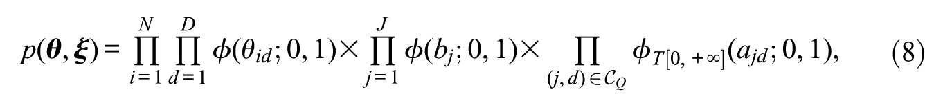
For the specification of prior joint distributions of the parameters of the M2PL-Q model, it is assumed that there is an independent prior structure, such that

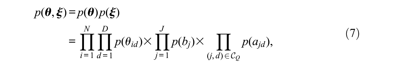
\begin{matrix} p (θ, ξ) = p (θ) p (ξ) \\ = Π_{i = 1}^{N} Π_{d = 1}^{D} p (θ_{id}) \times Π_{j = 1}^{J} p (b_{j}) \times \underset{(j, d) \in C_{Q}}{Π} p (a_{jd}), \end{matrix}

(7)

where $p (θ_{id})$ is the prior distributions of latent traits, $p (b_{j})$ is the prior distribution of difficulty parameters, $p (a_{jd})$ is the prior distribution of discrimination parameters, and $C_{Q} = {(j, d) : q_{jd} = 1, j = 1, 2, \dots, J, d = 1, 2, \dots, D} .$

Based on Curtis (2010), Bazán, Branco, and Bolfarine (2006), and Béguin and Glas (2001), we define the prior distributions for the parameters $a_{jd}$ , $b_{j}$ , and $θ_{id}$ as

\begin{matrix} a_{jd} ~ N (μ_{a}, σ_{a}) T [0, + \infty], for (j, d) \in C_{Q}; \\ b_{j} ~ N (μ_{b}, σ_{b}), for j = 1, 2, \dots, J; and \\ θ_{id} ~ N (μ_{θ}, σ_{θ}), for i = 1, 2, \dots, N and d = 1, 2, \dots, D, \end{matrix}

where $μ_{a}$ and $σ_{a}$ are the mean and the standard deviation of $a_{jd}$ ; $μ_{b}$ and $σ_{b}$ are the mean and the standard deviation of $b_{j}$ ; and $μ_{θ}$ and $σ_{θ}$ are the mean and standard deviation of $θ_{id}$ . The notation $N (μ, σ)$ indicates a normal distribution with mean $μ$ and standard deviation $σ$ and $T (0, + \infty)$ indicates that the distribution is truncated to include only positive values.

According to Béguin and Glas (2001), Fragoso and Cúri (2013), and Reckase (2009), to guarantee the identity of the M2PL model it is sufficient to set $μ_{θ} = 0$ . We also define $μ_{a} = μ_{b} = 0$ and $σ_{a} = σ_{b} = σ_{θ} = 1$ , and we use this setting for both the simulation study and for the application in this work. From the definition of the prior distributions and the hyperparameter values, we can rewrite Equation 7 as

\begin{matrix} p (θ, ξ) = Π_{i = 1}^{N} Π_{d = 1}^{D} ϕ (θ_{id}; 0, 1) \times Π_{j = 1}^{J} ϕ (b_{j}; 0, 1) \times \underset{(j, d) \in C_{Q}}{Π} ϕ_{T [0, + \infty]} (a_{jd}; 0, 1), \end{matrix}

(8)

where $ϕ (\cdot; 0, 1)$ is the standard normal probability density function and $ϕ_{T [0, + \infty]} (\cdot; 0, 1)$ is the truncated normal probability density function with mean equal to zero and standard deviation equal to 1.

The posterior distribution of the parameters of the M2PL-Q model, denoted by $p (θ, ξ | y)$ , is defined considering the likelihood in Equation 6 and the prior joint distribution in Equation 8, such that

\begin{matrix} p (θ, ξ | y) \propto ℓ (y | θ, ξ) \times p (θ, ξ) \\ = Π_{i = 1}^{N} [Π_{j = 1}^{J} P_{ij}^{w_{ij 1}} {(1 - P_{ij})}^{w_{ij 0}} \times Π_{d = 1}^{D} ϕ (θ_{id}; 0, 1)] \times Π_{j = 1}^{J} ϕ (b_{j}; 0, 1) \\ \times \underset{(j, d) \in C_{Q}}{Π} ϕ_{T [0, + \infty]} (a_{jd}; 0, 1) . \end{matrix}

(9)

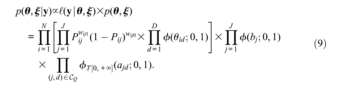
Since the posterior distribution given by Equation 9 has an intractable form, we use MCMC algorithms to obtain samples from it. Specifically, we chose to use an MCMC method called the No-U-Turn Sampler via Stan software (Carpenter et al., 2017), briefly described below.

NUTS Algorithm and Stan Software

The NUTS algorithm is an MCMC method developed by Hoffman and Gelman (2014) from the Hamiltonian Monte Carlo method (HMC) in order to construct a Markov chain more efficiently than other widely known MCMC methods used in Bayesian inference, such as Metropolis Hastings (Hastings 1970; Metropolis, Rosenbluth, Rosenbluth, Teller, & Teller, 1953) and Gibbs sampling (Gelfand & Smith, 1990; Geman & Geman, 1984). These methods use a probability distribution to construct a Markov chain and require a very large number of iterations. In contrast to Metropolis-Hastings and Gibbs sampling, HMC and consequently NUTS use Hamiltonian dynamics instead of a probability distribution to construct a Markov chain, making the simulation converge more quickly to the target distribution with low autocorrelation. The explanation of the NUTS algorithm can be found in Hoffman and Gelman (2014) and da Silva, de Oliveira, von Davier, and Bazán (2018).

In this article, we use NUTS via Stan software, a free and easy-to-use software, because it allows the user to write the statistical model similarly to BUGS software (Lunn, Thomas, Best, & Spiegelhalter, 2000) and JAGS software (Plummer, 2003), and it reproduces the C++ language model, compiles the code, executes the code, and produces an MCMC sample. We use Stan in the R software, through the RStan package (Stan Development Team, 2017).

Simulation Studies

In this section, we conducted two simulation studies using the M2PL-Q full, M2PL-Q bifac and M2PL-Q custom models. In the first study, we evaluated the parameter recovery of these three models using the NUTS algorithm in order to check the accuracy of the estimates of the parameters for the three Q-matrices considered. In the second study, we simulated a dataset using the M2PL-Q custom model, fitted the three models to this dataset and compared the estimates to the true values of the parameters, aiming to investigate the impact of the misspecified Q-matrix on the parameter estimates.

In both studies, we designed the Q-matrices to mirror a particular case taken from the data used in the application of this work and presented in the appendix. Specifically, the custom-Q was built for a 28-item English language test measuring three latent traits. Descriptions of this Q-matrix can be found in Buck and Tatsuoka (1998), Henson and Templin (2007), and Templin and Hoffman (2013). Similarly, for the full-Q and bifac-Q, we also fixed the number of items to $J = 28$ and the number of dimensions to $D = 3$ . Simulation studies with similar test lengths can be found in the literature, such as Azevedo, Bolfarine, and Andrade (2011).

Recovery of the Parameters

The values of discrimination and difficulty parameters were generated from a uniform distribution such that $a \in (0.25, 1.75)$ and $b \in (- 3, + 3)$ . Moreover, considering each of the Q-matrices, the values of the discrimination parameters were chosen such that $0.25 < MDIS C_{j} < 1.75$ , for $j = 1, 2, \dots, J$ . The constraint of the multidimensional discrimination parameter is necessary to obtain feasible values of the item discrimination parameters.

Based on Azevedo et al. (2011), we considered the sample size N as 500 and 1,000. Then, we simulated 10 replicate matrices of responses for each Q-matrix and we fit these replicas using 10,000 iterations in the NUTS algorithm, the first half being burn-in. This number is sufficient for the chains to converge using the NUTS algorithm. This was checked using the Gelman and Rubin diagnostic (Gelman & Rubin, 1992).

We considered some appropriate statistics to evaluate the parameter recovery of the M2PL-Q full, M2PL-Q bifac, and M2PL-Q custom models. The square root of the mean square error (RMSE) is the first statistic, given by

RMSE = \sqrt{\frac{1}{10} \sum_{r = 1}^{10} {({\hat{π}}_{lr} - π_{l})}^{2}},

where $π_{l}$ is an item or individual parameter, $l$ is a convenient index for the parameter, and ${\hat{π}}_{lr}$ is its respective estimate obtained in the replica $r$ , $r = 1, 2, \dots, 10$ . The second statistic is the absolute value of the relative bias (AVRB), given by

AVRB = \frac{| {\hat{\bar{π}}}_{l} - π_{l} |}{| π_{l} |},

where ${\hat{\bar{π}}}_{l} = \frac{1}{10} \sum_{r = 1}^{10} {\hat{π}}_{lr} .$

Table 2 shows the RMSE values for the items’ parameter estimates for the two scenarios constructed from the different sample sizes considered in each model. We also present in Table 2 the average correlations between ${\hat{π}}_{lr}$ and $π_{l}$ , that is, the mean correlation between the parameter estimates and their corresponding true values. In addition, we added the average execution time of the NUTS algorithm to fit the models.

Table 2.

Average RMSE Values and Average Correlations for the Parameters of the Items and the Average Execution Time, in Seconds.

M2PL-Q models	N	RMSE				Correlation				Time
M2PL-Q models	N	$a_{j 1}$	$a_{j 2}$	$a_{j 3}$	$b_{j}$	$a_{j 1}$	$a_{j 2}$	$a_{j 3}$	$b_{j}$	Time
Full	500	$. 136$	$. 135$	$. 153$	$. 194$	$. 860$	$. 851$	$. 814$	$. 993$	2,353
Full	1,000	$. 112$	$. 107$	$. 130$	$. 113$	$. 860$	$. 880$	$. 861$	$. 996$	6,305
Bifac	500	$. 203$	$. 226$	$. 330$	$. 113$	$. 900$	$. 839$	$. 826$	$. 994$	985
	1,000	$. 158$	$. 199$	$. 246$	$. 085$	$. 934$	$. 871$	$. 939$	$. 997$	3,012
Custom	500	$. 215$	$. 267$	$. 178$	$. 113$	$. 939$	$. 967$	$. 961$	$. 994$	662
	1,000	$. 170$	$. 301$	$. 150$	$. 086$	$. 970$	$. 973$	$. 973$	$. 996$	1,847

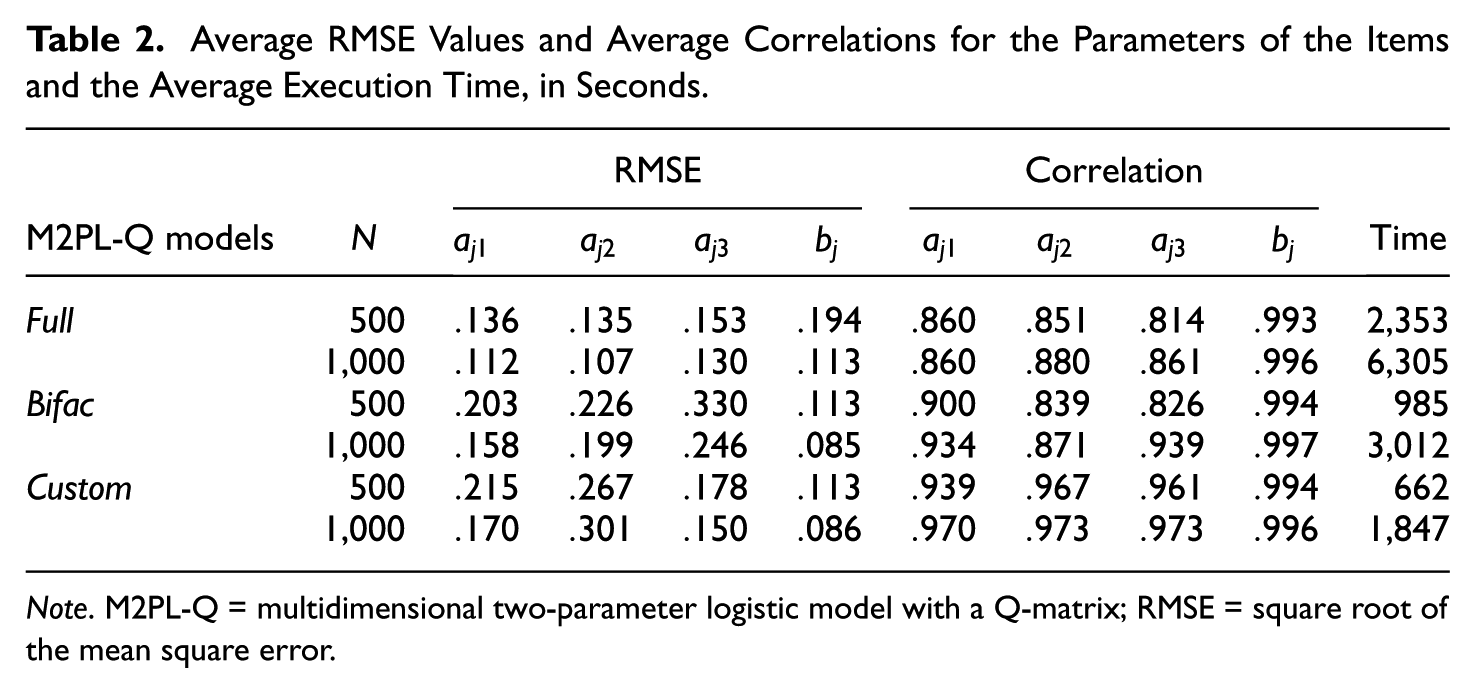
Note. M2PL-Q = multidimensional two-parameter logistic model with a Q-matrix; RMSE = square root of the mean square error.

We can visualize that by increasing the N value from 500 to 1,000, the RMSE values for the parameters decreased in almost all cases, except for the parameter $a_{j 2}$ in the M2PL-Q custom model, which had larger RMSE values. An increase in the value of N also caused the values of the correlations to increase, except for the parameter $a_{j 1}$ in the M2PL-Q full model. In addition, the 100% increase in the number of individuals made the computational time of the NUTS algorithm increase more than 2.5 times in the three models.

The AVRB values are presented in boxplot format in Figure 1. The first graph refers to the M2PL-Q full model, the second refers to the M2PL-Q bifac model, and the third refers to M2PL-Q custom model. In each graph, there are four boxplots referring to the items’ parameter estimates for the two sample sizes considered.

Figure 1.

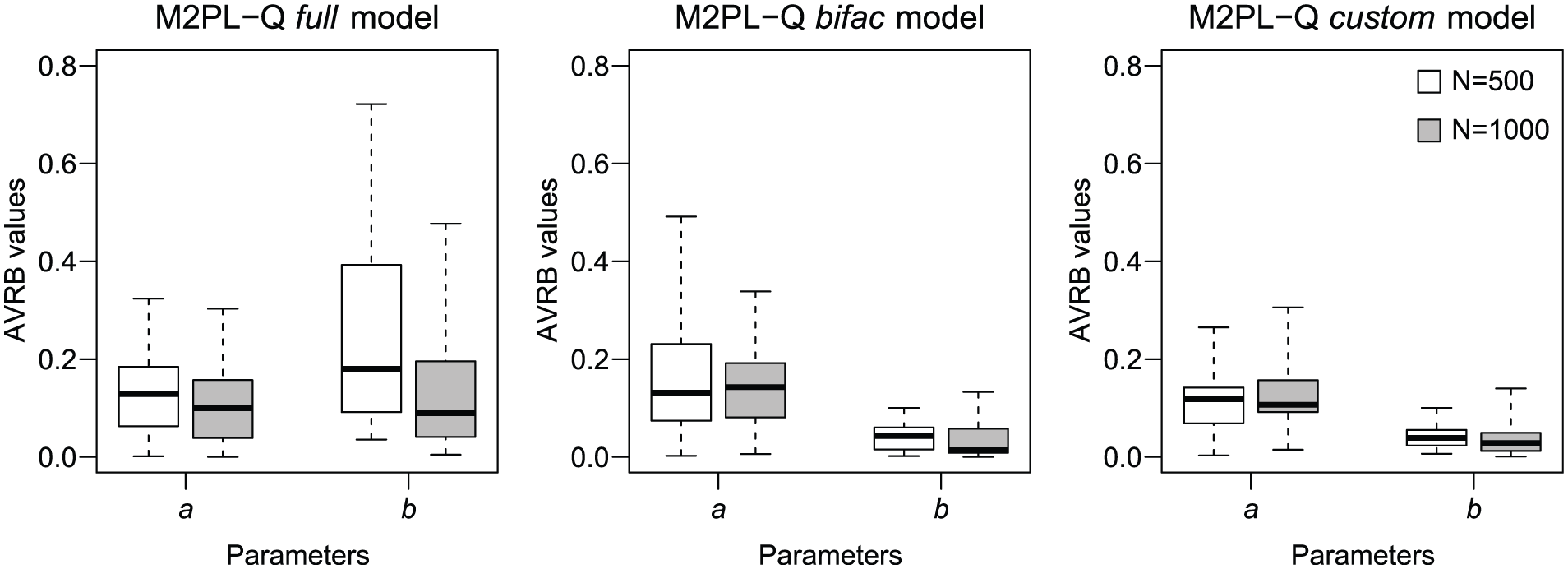
The AVRB values of the discrimination, difficulty, and individual parameters for the three models considered in this simulation study.

In the three models considered, the AVRB values are considered small. In general, the increase in the number of individuals does not appear to have influenced the AVRB values considerably.

Parameter Estimates of M2PL-Q Model for Misspecified Q-Matrices The M2PL-Q Model

In this study, we compared the estimated and true values of the discrimination, difficulty, and individuals’ parameters for the M2PL-Q full, M2PL-Q bifac, and M2PL-Q custom models. We used the same parameter values generated in the previous study to simulate a response matrix from the M2PL-Q custom model, to which the three models were fit. These three models were defined using the full-Q, bifac-Q, and custom-Q matrices, as specified in Section. Each of these matrices has a concept behind it, considering test characteristics and latent traits of interest. Primarily, this is taken into consideration by content experts.

Discrimination Parameters

The four graphs presented in Figure 2 refer to the estimates of the discrimination parameters of the M2PL-Q full, M2PL-Q bifac, and M2PL-Q custom models. In addition, the true values of the discrimination parameters used in the simulation of the response matrix from the the M2PL-Q custom model are presented. The first three graphs show the discrimination values associated with Dimensions 1, 2, and 3 corresponding to the M2PL-Q custom model, while the fourth graph shows the values of multidimensional discrimination.

Figure 2.

The first three graphs present the true values for each dimension of the discrimination parameters and the estimates of these parameters found from the M2PL-Q full, M2PL-Q bifac, and M2PL-Q custom models. The last graph presents the multidimensional discrimination calculated from Equation 4 for the true values and for the estimates of the parameters considering the three models.

In general, the estimates of the dimension-specific discrimination parameters of the M2PL-Q custom model were closer to their true values in than were the estimates of those discrimination parameters of the M2PL-Q full and M2PL-Q bifac models, as expected. Considering the fourth graph, the estimates of the multidimensional discriminations were notably closer to their true values than the estimates of dimension-specific discriminations, and estimates of the M2PL-Q custom model were slightly closer to their true values than the estimates of the other two models.

Difficulty Parameters

The four graphs presented in Figure 3 compare the estimates of the difficulty parameters of the M2PL-Q full, M2PL-Q bifac, and M2PL-Q custom models to their true values. The first three graphs present the true values of the difficulty parameters against their estimates from each of the three models, while the fourth graph presents via boxplots the absolute value distributions of the differences between estimates and true values in each model.

Figure 3.

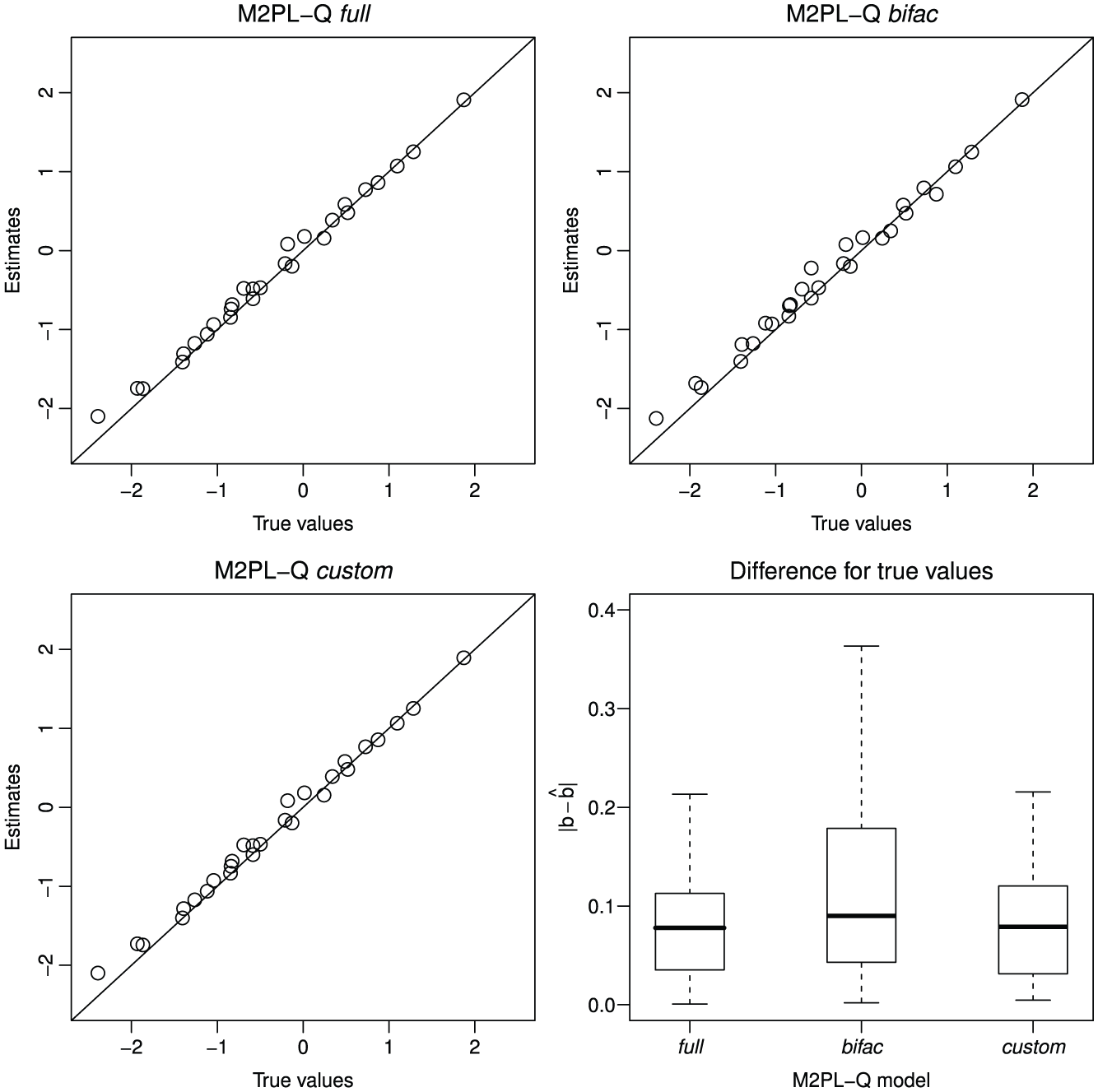
The first three graphs present a comparison between the true values of the difficulty parameters and the estimates of these parameters found from the M2PL-Q full, M2PL-Q bifac, and M2PL-Q custom models. The last graph presents one boxplot for each model with the differences between true values and estimates of the difficulty parameters.

All difficulty parameters were appropriately estimated using the three models. Although the graphs show that the M2PL-Q bifac model was the worst case, we can still consider those estimates as acceptable.

Individuals’ Parameters

We present in Figure 4 three graphs to compare the estimates of the latent traits to their true values. Each graph refers to a dimension of the individuals’ parameters and contains three boxplots representing the distribution of the absolute values of the difference between estimates and true values.

Figure 4.

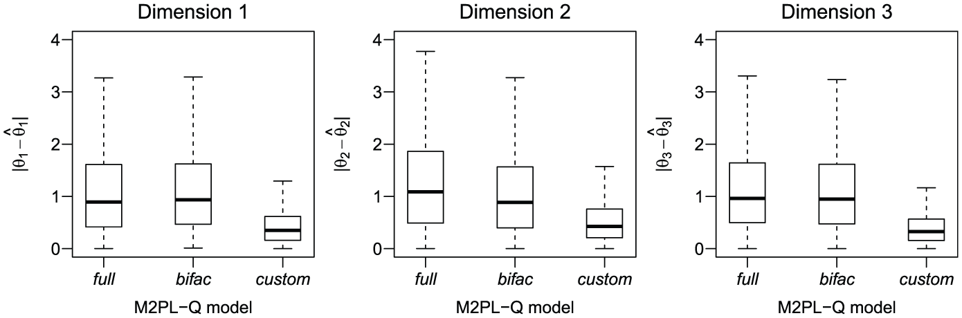
The three graphs present one boxplot for each model with the differences between true values and estimates of the individuals’ parameters.

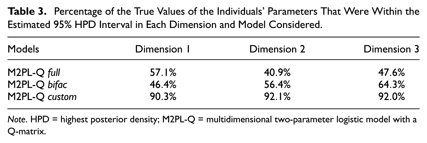
Considering the three dimensions, the distributions of the absolute values of the differences between estimates and their true values are similar for the M2PL-Q full and M2PL-Q bifac models. However, the absolute values of the differences between estimates and their true values from the M2PL-Q custom model are smaller in the three dimensions, indicating as expected that the M2PL-Q custom model is the most appropriate for the data. To make this clear, we estimated a 95% highest posterior density (HPD) interval for each latent trait from each model and checked how many contained the true value of the corresponding parameter. Table 3 contains the percentage of true values of the individuals’ parameters that were contained in these intervals for each dimension and model.

Table 3.

Percentage of the True Values of the Individuals’ Parameters That Were Within the Estimated 95% HPD Interval in Each Dimension and Model Considered.

Models	Dimension 1	Dimension 2	Dimension 3
M2PL-Q full	57.1%	40.9%	47.6%
M2PL-Q bifac	46.4%	56.4%	64.3%
M2PL-Q custom	90.3%	92.1%	92.0%

Note. HPD = highest posterior density; M2PL-Q = multidimensional two-parameter logistic model with a Q-matrix.

Considering the individuals’ parameters on Dimension 1, the HPD intervals constructed from the M2PL-Q full model contain 57.1% of their true values. Considering this interpretation for the other percentages presented in Table 3, these values indicate that, among the three models compared, only the M2PL-Q custom model is adequate to estimate latent traits from the simulated data. Again, this result demonstrates expected findings.

Application

In this section, we conducted an application with real data of English proficiency measures in order to illustrate the use of the M2PL-Q model in practical problems.

Description of the Data

We used a dataset with 2,922 individuals who answered 28 items on the Examination for the Certificate of Proficiency in English (ECPE). Written permission to use this dataset was obtained from the Cambridge Michigan Language Assessments (CaMLA). The ECPE is designed to measure the English language skills for nonnative English speakers. The 28 items on the ECPE were designed to measure three skills: “knowledge of (1) morphosyntactic rules, (2) cohesive rules, and (3) lexical rules” (see Templin & Hoffman 2013).

We fit the data to the M2PL-Q model with three different Q-matrices: (1) the oneD-Q matrix, defined as the unit vector $(1, 1, \dots, 1)'$ of 28 elements, transforming the model M2PL-Q into the one-dimensional 2PL model to verify the adequacy of the data in the one-dimensionality assumption; (2) the custom-Q matrix, defined by an expert in the field of the construct of measurement and used in the simulation study; and (3) the custom-global-Q matrix, which was formed by adding an extra column of 1s to the custom-Q matrix to represent a global latent trait. Note in this third case that we did not fit a bifactor model because, although we have a global latent trait, there are items that are influenced by more than two specific latent traits. The custom-Q and custom-global-Q are presented in the appendix to this article.

Setting the Fit of the M2PL-Q Model

The 2PL, M2PL-Q custom, and M2PL-Q custom-global models were fit to the data using the NUTS algorithm via Stan software. We used 10,000 iterations, the first half being burn-in and therefore discarded. The convergence of the posterior distributions of the parameters in both models was checked from the Gelman and Rubin Convergence Diagnostic (Gelman & Rubin, 1992).

Main Results

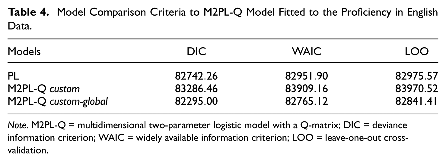
In order to verify which model was most appropriate to the Proficiency in English data, we present in Table 4 the values of three model comparison criteria considered in this study: deviance information criterion (DIC; Spiegelhalter, Best, Carlin, & van der Linden, 2002), widely available information criterion (WAIC; Watanabe, 2010), and leave-one-out cross-validation criterion (known by LOO; Vehtari, Gelman, & Gabry, 2017).

Table 4.

Model Comparison Criteria to M2PL-Q Model Fitted to the Proficiency in English Data.

Models	DIC	WAIC	LOO
PL	$82742.26$	$82951.90$	$82975.57$
M2PL-Q custom	$83286.46$	$83909.16$	$83970.52$
M2PL-Q custom-global	$82295.00$	$82765.12$	$82841.41$

Note. M2PL-Q = multidimensional two-parameter logistic model with a Q-matrix; DIC = deviance information criterion; WAIC = widely available information criterion; LOO = leave-one-out cross-validation.

From the values of the fit indices, we considered the M2PL-Q custom-global model for data analysis. We present in Figure 5 estimates of discrimination parameters, in Figure 6 estimates of difficulty parameters, and in Figure 7 estimates of individual parameters.

Figure 5.

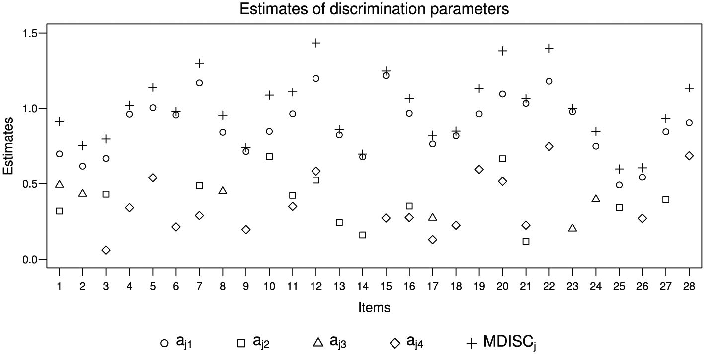
Estimates of global, specific, and multidimensional (MDISC) discrimination’s parameters considering the latent traits evaluated from M2PL-Q custom-global model.

Figure 6.

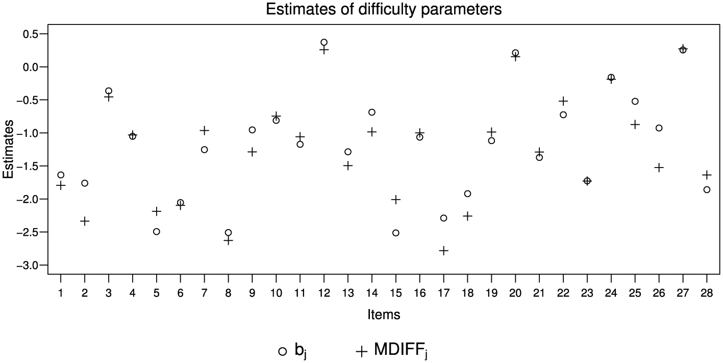
Estimates of difficulty’s parameters and multidimensional difficulty (MDIFF) parameters from M2PL-Q custom-global model.

Figure 7.

Summary of estimates of individuals’ parameters.

Estimates of global discrimination parameters were larger than estimates of domain-specific discrimination parameters in all items, indicating that the items better distinguished individuals in terms of the global latent trait than the specific latent traits. Some items had estimates of one of the domain-specific discriminations close to zero, such as Item 3 ( $a_{3, 4} = 0.06$ ), Item 17 ( $a_{17, 4} = 0.13$ ), and Item 21 ( $a_{21, 2} = 0.12$ ), making the influence of their respective latent traits insignificant for the individual’s response to these items.

In general, the estimates of the difficulty parameters were small, indicating that the probabilities of individuals scoring correctly on items were high even for those low on the latent traits.

Furthermore, in the one-dimensional 2PL model, the difficulty parameter related to an item corresponds to the value of the latent trait necessary for a .50 probability of correct item response. As in the M2PL-Q model, the difficulty parameters cannot be interpreted in the same way as they are in the one-dimensional 2PL model (Reckase, 2009). However, as in the one-dimensional model, $b_{j}$ continues to be defined as the difficulty for an individual scoring correctly on item $j$ . For example, the estimation of parameter $b_{12}$ is $0.37$ and is interpreted as the difficulty for an individual scoring correctly on Item 12.

The mean of the estimates of individuals’ parameters in the four dimensions is close to zero. The standard deviation of the global dimension is higher than in the other dimensions, with a value equal to 0.83. In contrast, the standard deviation of Dimension 2 (Cohesive rules) is the smallest, with a value equal to 0.3.

Conclusions

In this article, we incorporated the Q-matrix into the traditional formulation of the M2PL model and we call it the M2PL-Q. This provides an efficient way of including item specification mathematically, considering expert opinions and prior knowledge available. Also, this M2PL-Q model enables the construction of a link between MIRT models and DCMs. In this section, we summarize the findings of the simulation and applied studies, discuss the properties of the proposed model, and offer future research directions.

The first simulation study, designed to evaluate the recovery of parameters from the M2PL-Q model using different Q-matrices, showed that the estimation method used provides good results for all evaluated cases. As expected, the precision of the estimates improves with increased sample sizes.

The next simulation study was formulated to compare the estimates of the M2PL-Q full, M2PL-Q bifac, and M2PL-Q custom models and the true values of the parameters, considering a simulated dataset from the M2PL-Q custom model. That is, we aimed to investigate the impact of the Q-matrix (mis)specification on the parameter estimates. As we expected, the estimates of the discrimination and individual parameters of the M2PL-Q custom model were closer to their true values than the estimates obtained by the other models. However, the estimates of the difficulty parameters of the M2PL-Q custom model were close to their true values as well as the estimates of the difficulty parameters obtained by the M2PL-Q bifac model and M2PL-Q full model. This indicates that the constraints on the M2PL-Q model do not considerably influence the estimates of the difficulty parameters, although they did considerably affect the estimates of the discrimination and individual parameters.

The application study demonstrated the utility of the proposed model in practice. Here we briefly summarize the steps for practitioners to use the M2PL-Q in operational settings.

Step 1: Specify the item-trait relationship into the Q-matrix.

Step 2: Fit one or more specified M2PL-Q model(s) to the item responses.

Step 3: Evaluate fit indices, dimensionality, and reliability.

Step 4: Examine the discrimination, difficulty and individuals’ parameter estimates.

Step 5: Select models and make changes to the Q-matrix if necessary.

Similar to fitting other psychometric models to item responses, the steps are iterative in nature. After Step 5, one may or may not need to go back to Step 1 in order to specify a new Q-matrix utilizing information from the model-fitting process.

Incorporating the Q-matrix into the composition of IRT models provides some practical benefits. First, relationships between items and latent traits can be specified directly during test development and incorporated into the model through the Q-matrix in a user-friendly manner, which helps education, psychology, or other field experts to easily manipulate these models and insert the restrictions on the relationships between items and latent traits. In addition, these constraints provided by the Q-matrix decrease the number of discrimination parameters of the model, simplify the estimation process, increase the accuracy of latent trait estimates, and considerably shorten the estimation time as compared to a fully unrestricted MIRT (identical to M2PL-Q full). However, we want to point out that the Q-matrix is not a panacea for estimation burdens. The complexity of the Q-matrix, which often is defined by content experts, determines whether the number of parameters can be reduced. Therefore, in practice, greater care is required for the IRT models that incorporate Q-matrices. Information in the literature and empirical support are of great importance for the construction of the Q-matrix. This can be considered a disadvantage of the model proposed in this work.

Future work can be developed in order to extend the proposal of this article. First, other multidimensional IRT models, such as multidimensional 1PL and 3PL models, and models for polytomous items discussed in Reckase (2009), can incorporate the Q-matrix in a similar fashion to the M2PL-Q model proposed in this work. The impact of a Q-matrix specification on these new models can be investigated. Second, incorrect specification of a Q-matrix has been demonstrated to affect parameter estimation, result in poor model fit, and decrease classification accuracy in DCMs (e.g., Gao, Miller, & Liu, 2017; Kunina-Habenicht, Rupp, & Wilhelm, 2012; Liu, 2017; Rupp & Templin, 2008a). Therefore, it would be helpful to explore the effects of Q-matrix specification on the estimation of MIRT model parameters. Third, future research can explore the possibilities of defining a Q-matrix through data validation in MIRT models. Fourth, methods have been proposed about using the item responses to validate the Q-matrix under DCMs (e.g., De La Torre, 2008; De La Torre & Chiu, 2016; Wang et al., 2018). Those methods may shed light on how to recover the true item–trait relationship in MIRT. Fifth, a prior sensitivity study on models that incorporated the Q-matrix is needed when using our proposed estimation method, including cases such as nonnormality of latent traits, as in Azevedo et al. (2011), and asymmetry of link functions, as in Bazán et al. (2006). With the introduction of Q-matrices embedded in MIRT models and the suggestions for future research, we hope this idea will eventually allow for more accurate estimates of individuals’ multiple latent traits through assessments.

Footnotes

Appendix

This appendix presents the Full-Q, Bifac-Q, Custom-Q, and Custom-Global-Q Matrices Used in the Simulation Studies and Application of This Article.

Declaration of Conflicting Interests

The author(s) declared no potential conflicts of interest with respect to the research, authorship, and/or publication of this article.

Funding

The author(s) disclosed receipt of the following financial support for the research, authorship, and/or publication of this article: This study was financed in part by the Coordenação de Aperfeioamento de Pessoal de Nível Superior - Brasil (CAPES) - Finance Code 001. The fourth author was partially supported by the Brazilian agency FAPESP (Grant 2017/15452-5).

ORCID iDs

Marcelo A. da Silva

Ren Liu

References

Ackerman

(1994). Using multidimensional item response theory to understand what items and tests are measuring. Applied Measurement in Education, 7, 255-278. doi:10.1207/s15324818ame0704\_1

Ackerman

(1996). Graphical representation of multidimensional item response theory analyses. Applied Psychological Measurement, 20, 311-329. doi:10.1177/014662169602000402

Azevedo

Bolfarine

Andrade

(2011). Bayesian inference for a skew-normal IRT model under the centred parameterization. Computational Statistics and Data Analysis, 55, 353-365. doi:10.1016/j.csda.2010.05.003

Bazán

Branco

Bolfarine

(2006). A skew item response model. Bayesian Analysis, 1, 861-892. doi:10.1214/06-BA128

Béguin

Glas

(2001). MCMC estimation and some model-fit analysis of multidimensional IRT models. Psychometrika, 66, 541-561. doi:10.1007/BF02296195

Buck

Tatsuoka

(1998). Application of the rule-space procedure to language testing: Examining attributes of a free response listening test. Language Testing, 15, 119-157. doi:10.1177/026553229801500201.

Carpenter

Gelman

Hoffman

Lee

Goodrich

Betancourt

. . . Riddell

. (2017). Stan: A probabilistic programming language. Journal of Statistical Software, 76(1), 1-32. doi:10.18637/jss.v076.i01

Curtis

(2010). Bugs code for item response theory. Journal of Statistical Software, 36(1), 1-34. doi:10.18637/jss.v036.c01

da Silva

de Oliveira

von Davier

Bazán

. (2018). Estimating the Dina model parameters using the No-U-Turn Sampler. Biometrical Journal, 60, 352-368. doi:10.1002/bimj.201600225

10.

De La Torre

(2008). An empirically based method of Q-matrix validation for the Dina model: Development and applications. Journal of Educational Measurement, 45, 343-362. doi:10.1111/j.1745-3984.2008.00069.x

11.

De La Torre

Chiu

(2016). A general method of empirical Q-matrix validation. Psychometrika, 81, 253-273. doi:10.1007/s11336-015-9467-8

12.

Drasgow

Parsons

(1983). Application of unidimensional item response theory models to multidimensional data. Applied Psychological Measurement, 7, 189-199. doi:10.1177/014662168300700207

13.

Fragoso

Cúri

(2013). Improving psychometric assessment of the Beck Depression Inventory using multidimensional item response theory. Biometrical Journal, 55, 527-540. doi:10.1002/bimj.201200197

14.

Gao

Miller

Liu

(2017). The impact of Q-matrix misspecification and model misuse on classification accuracy in the generalized Dina model. Journal of Measurement and Evaluation in Education and Psychology, 8, 391-403. doi:10.21031/epod.332712

15.

Gelfand

Smith

(1990). Sampling-based approaches to calculating marginal densities. Journal of the American Statistical Association, 85, 398-409. doi:10.2307/2289776

16.

Gelman

Rubin

(1992). Inference from iterative simulation using multiple sequences. Statistical Science, 7, 457-472. doi:10.1214/ss/1177011136

17.

Geman

(1984). Stochastic relaxation, Gibbs distributions and the Bayesian restoration of images. IEEE Transactions on Pattern Analysis and Machine Intelligence, 6, 721-741. doi:10.1109/TPAMI.1984.4767596

18.

Gibbons

Hedeker

(1992). Full-information item bi-factor analysis. Psychometrika, 57, 423-436. doi:10.1007/BF02295430

19.

Haberman

Sinharay

(2010). Reporting of subscores using multidimensional item response theory. Psychometrika, 75, 209-227. doi:10.1007/s11336-010-9158-4

20.

Hastings

(1970). Monte Carlo sampling methods using Markov chains and their applications. Biometrika, 57, 97-109. doi:10.2307/2334940

21.

Henson

Templin

(2007). Large-scale language assessment using cognitive diagnosis models. Paper presented at the Annual meeting of the National Council for Measurement in Education, Chicago, IL.

22.

Hoffman

Gelman

(2014). The No-U-Turn Sampler: Adaptively setting path lengths in Hamiltonian Monte Carlo. Journal of Machine Learning Research, 15, 1593-1623.

23.

Kunina-Habenicht

Rupp

Wilhelm

(2012). The impact of model misspecification on parameter estimation and item-fit assessment in log linear diagnostic classification models. Journal of Educational Measurement, 49, 59-81. doi:10.1111/j.1745-3984.2011.00160.x

24.

Liu

(2017). Misspecification of attribute structure in diagnostic measurement. Educational and Psychological Measurement, 78, 605-634.

25.

Liu

Huggins-Manley

A. C.

Bradshaw

(2016). The impact of Q-matrix designs on diagnostic classification accuracy in the presence of attribute hierarchies. Educational and Psychological Measurement, 77, 220-240. doi:10.1177/0013164416645636

26.

Liu

Huggins-Manley

A. C.

Bulut

(2018). Retrofitting diagnostic classification models to responses from IRT-based assessment forms. Educational and Psychological Measurement, 78, 357-383. doi:10.1177/0013164416685599

27.

Liu

Qian

Luo

Woo

(2017). Relative diagnostic profile: A subscore reporting framework. Educational and Psychological Measurement, 78, 1072-1088.

28.

Lord

Novick

(1968). Statistical theories of mental test scores. Menlo Park, CA: Addison-Wesley.

29.

Lunn

D. J.

Thomas

Best

Spiegelhalter

(2000). Winbugs—a Bayesian modelling framework: Concepts, structure, and extensibility. Statistics and Computing, 10, 325-337. doi:10.1023/A:1008929526011

30.

Madison

Bradshaw

(2015). The effects of Q-matrix design on classification accuracy in the log-linear cognitive diagnosis mode. Educational and Psychological Measurement, 75, 491-511.

31.

Maydeu-Olivares

(2001). Multidimensional item response theory modeling of binary data: Large sample properties of noharm estimates. Journal of Educational and Behavioral Statistics, 26, 51-71. doi:10.3102/10769986026001051

32.

Metropolis

Rosenbluth

Teller

(1953). Equation of state calculations by fast computing machines. Journal of Chemical Physics, 21, 1087-1092. doi:10.1063/1.1699114

33.

Plummer

(2003, March). Jags: A program for analysis of Bayesian graphical models using Gibbs sampling. Paper presented at the 3rd International Workshop on Distributed Statistical Computing (DSC 2003), Vienna, Austria.

34.

Reckase

(1985). The difficulty of test items that measure more than one ability. Applied Psychological Measurement, 9, 401-412. doi:10.1177/014662168500900409

35.

Reckase

(2009). Multidimensional item response theory. Berlin, Germany: Springer.

36.

Rupp

Templin

(2008a). The effects of Q-matrix misspecification on parameter estimates and classification accuracy in the Dina model. Educational and Psychological Measurement, 68, 78-96. doi:10.1177/0013164407301545

37.

Rupp

Templin

(2008b). Unique characteristics of diagnostic classification models: A comprehensive review of the current state-of-the-art. Measurement, 6, 210-262.

38.

Rupp

Templin

Henson

(2010). Diagnostic measurement: Theory, methods, and applications. New York, NY: Guilford Press.

39.

Spiegelhalter

D. J.

Best

N. G.

Carlin

B. P.

van der Linden

(2002). Bayesian measures of model complexity and fit. Journal Royal Statistical Society, Series B, 64, 583-639.

40.

Stan Development Team. (2017). Rstan: The R interface to Stan. Retrieved from http://mc-stan.org

41.

Tatsuoka

(1983). Rule space: An approach for dealing with misconceptions based on item response theory. Journal of Educational Measurement, 20, 345-354. doi:10.1111/j.1745- 3984.1983.tb00212.x

42.

Templin

Bradshaw

(2013). Measuring the reliability of diagnostic classification model examinee estimates. Journal of Classification, 30, 251-275. doi:10.1007/s00357- 013-9129-4

43.

Templin

Hoffman

(2013). Obtaining diagnostic classification model estimates using Mplus. Educational Measurement: Issues and Practice, 32(2), 37-50. doi:10.1111/emip.12010

44.

Thissen

(2016). Bad questions: An essay involving item response theory. Journal of Educational and Behavioral Statistics, 41, 81-89. doi:10.3102/1076998615621300

45.

Vehtari

Gelman

Gabry

(2017). Practical Bayesian model evaluation using leave-one-out cross-validation and WAIC. Statistics and Computing, 27, 1413-1432. doi:10.1007/s11222-016-9696-4

46.

Wang

Song

Ding

Meng

Cao

Jie

(2018). An EM-based method for Q-matrix validation. Applied Psychological Measurement, 42, 446-459. doi:10.1177/0146621617752991

47.

Watanabe

(2010). Asymptotic equivalence of Bayes cross validation and widely applicable information criterion in singular learning theory. Journal of Machine Learning Research, 11, 3571-3594.