On the Pitfalls of Estimating and Using Standardized Reliability Coefficients

Abstract

The population discrepancy between unstandardized and standardized reliability of homogeneous multicomponent measuring instruments is examined. Within a latent variable modeling framework, it is shown that the standardized reliability coefficient for unidimensional scales can be markedly higher than the corresponding unstandardized reliability coefficient, or alternatively substantially lower than the latter. Based on these findings, it is recommended that scholars avoid estimating, reporting, interpreting, or using standardized scale reliability coefficients in empirical research, unless they have strong reasons to consider standardizing the original components of utilized scales.

Keywords

congeneric tests congeneric test model measuring instrument reliability single-factor model standardized reliability coefficient unstandardized reliability coefficient

Multiple component measuring instruments are highly popular in the behavioral, social, marketing, business, clinical, and educational sciences (e.g., Raykov & Marcoulides, 2011). An index that is commonly used to reflect the quality of these measurement devices is the reliability coefficient, which has received a great deal of attention over the past several decades by methodologists and substantive scholars (e.g., McDonald, 1999). In the empirical research literature, a particular version of instrument (scale) reliability that has been frequently used is the so-called standardized reliability coefficient. This coefficient has been at times employed instead of the regular (unstandardized) reliability coefficient, likely due in part to the straightforward availability of standardized reliability indices in widely circulated software such as SPSS, SAS, or Stata (cf. McNeish, 2018; see also Raykov & Marcoulides, 2019). Unfortunately, the standardized reliability coefficient can be spuriously high, or alternatively spuriously low, and thus, seriously mislead researchers about the relevant, actual measurement quality level of an instrument under consideration.¹

The present note is concerned with the potential pitfalls that a scholar may encounter if estimating, utilizing, reporting or interpreting standardized reliability coefficients and subsequently justifying decisions related to scales under consideration based on these coefficients. For the widely used setting of a unidimensional multicomponent measuring instrument, the population discrepancy between the corresponding standardized and unstandardized reliability coefficients is of particular interest in the remainder of this article. The following discussion shows that the population standardized reliability of a homogeneous scale with uncorrelated errors can be markedly higher or substantially lower than its unstandardized (ordinary, traditional, conventional, regular) scale reliability counterpart. Therefore, scientists employing, estimating, providing, reporting, and/or interpreting the standardized reliability coefficient in their work may in fact (a) end up promoting lower quality scales that possess deficient actual reliability (and possibly validity) than that reflected in their spuriously high standardized coefficient; or, alternatively, (b) miss a scale (version) with what might be considered “satisfactory” reliability, by being pre-occupied with its notably inferior standardized reliability coefficient. Based on these findings, the article also aims to recommend generally to avoid estimating, employing, reporting, or interpreting standardized scale reliability estimates, unless researchers have strong reasons for using the standardized original scale components.

Background, Notation, and Assumptions

This note develops within the framework of classical test theory (e.g., Zimmerman, 1975), and specifically that of the congeneric test model (which in the setting of concern is equivalent to, i.e., empirically indistinguishable from, the highly popular single-factor model; e.g., Jöreskog, 1971). Suppose X₁, X₂, . . ., X_k (k > 2) denote the k (approximately) continuous components of a unidimensional measuring instrument of interest (e.g., Raykov & Marcoulides, 2011). For example, these can be the k subtests in a given test battery, or the scores on k testlets within a longer measuring instrument (generically referred to as “scale” in what follows). We make also the frequently advanced assumption that this scale is used in a single-level, single-class population of concern (i.e., a population with no clustering effects and consisting of a single as opposed to multiple latent classes; e.g., Raykov et al., 2016).

In empirical research, frequently the reliability of the sum score

Y = X_{1} + X_{2} + \dots + X_{k}

(1)

is of particular interest (often referred to as “scale score”). In the congeneric tests case,

X_{j} = a_{j} + b_{j} T + E_{j}

(2)

holds, where T is the common underlying true score, a_j the pertinent intercept, b_j the loading of T on X_j, and E_j the associated measurement error (j = 1, . . ., k; Jöreskog, 1971). In the rest of this discussion, we presume that the error terms are uncorrelated, as well as that b_j > 0 and Var(T) = 1, which are constraints that entail empirically no loss of generality; further, µ(T) = 0 is similarly set for identifiability reasons, with Var(·) and µ(·) denoting variance and mean, respectively (j = 1, . . ., k).

Within this setting oftentimes of special theoretical and empirical relevance in behavioral, social, educational, marketing, business, and clinical research, the remainder of the present article (a) is concerned with the population difference between the unstandardized and standardized reliability coefficients and (b) demonstrates that the standardized reliability coefficient can be markedly higher than its unstandardized counterpart—or alternatively substantially inferior to it—already at the population level.

The Population Discrepancy Between the Unstandardized and Standardized Reliability Coefficients

Standardized and Unstandardized Reliability as Functions of Model Parameters

From Equations (1) and (2), it follows that the reliability coefficient of the sum score Y, denoted by ρ_Y and defined as the ratio of its true variance to observed variance, is

ρ_{Y} = (b_{1} + \dots + b_{k})^{2} / [(b_{1} + \dots + b_{k})^{2} + v_{1} + \dots + v_{k}],

(3)

where the v’s denote the respective variances of the E’s (e.g., Raykov, 2012; in this article all formulas used involve only population parameters, unless stated otherwise). The coefficient in Equation (3) represents the (regular, ordinary, “standard,” traditional, or conventional) population scale reliability, and is referred to in the remainder as “unstandardized scale reliability,”“scale reliability coefficient,” or simply “scale reliability.”

The standardized scale reliability is defined as the reliability coefficient of the sum of the z-scores associated with the original scale components,

Z_{j} = [X_{j} - μ (X_{j})] / \sqrt{Var (X_{j})},

(4)

where a positive square root is taken in the denominator (j = 1, . . ., k; cf. McDonald, 1999). That is, the standardized reliability coefficient associated with the scale consisting of the components X₁, . . ., X_k, is the reliability coefficient of the sum score Z = Z₁+Z₂+⋯+Z_k, denoted as ρ_Z, which equals

ρ_{Z} = Var (T_{Z}) / Var (Z),

(5)

where T_Z is the true score of Z (see also Appendix A; the quantity (5) will be also referred to in the remainder as “standardized scale reliability,”“standardized reliability coefficient,” or simply “standardized reliability”). Appendix A shows that in terms of the parameters of the congeneric test model (1),

\begin{matrix} ρ_{z} = \frac{{(\sum_{j = 1}^{k} \frac{b_{j}}{\sqrt{{b_{j}}^{2} + v_{j}}})}^{2}}{{(\sum_{j = 1}^{k} \frac{b_{j}}{\sqrt{{b_{j}}^{2} + v_{j}}})}^{2} + \sum_{j = 1}^{k} \frac{v_{j}}{{b_{j}}^{2} + v_{j}}} \\ = 1 / (1 + B) \end{matrix}

(6)

holds, with

B = \frac{\sum_{j = 1}^{k} \frac{v_{j}}{{b_{j}}^{2} + v_{j}}}{{(\sum_{j = 1}^{k} \frac{b_{j}}{\sqrt{{b_{j}}^{2} + v_{j}}})}^{2}} .

(7)

(Note that the denominator of B, that of expression A in Equation 9, and the right-hand side of Equation 3 are all positive, owing to the earlier made assumption of positive loadings b_j, j = 1, . . ., k.)

By analogy to the developments in Appendix A, and based on Equation (3), the scale reliability coefficient can be expressed with straightforward algebra as

ρ_{Y} = 1 / (1 + A),

(8)

where

A = \frac{\sum_{j = 1}^{k} v_{j}}{{(\sum_{j = 1}^{k} b_{j})}^{2}} .

(9)

From Equations (6) and (8) it follows that the population discrepancy between the standardized reliability and scale reliability coefficients, denoted as Δ, is (see also Equations 7 and 9)

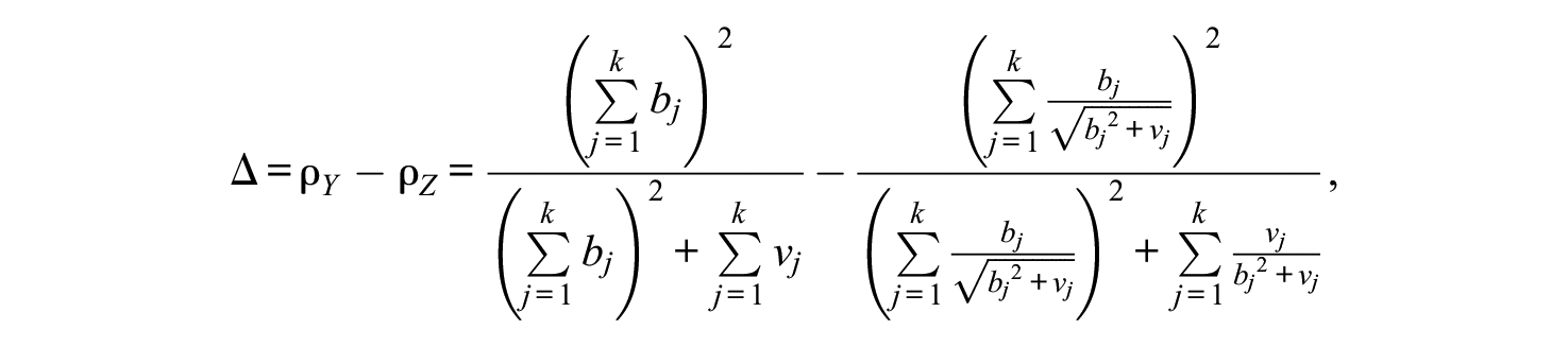
Δ = ρ_{Y} - ρ_{Z} = \frac{{(\sum_{j = 1}^{k} b_{j})}^{2}}{{(\sum_{j = 1}^{k} b_{j})}^{2} + \sum_{j = 1}^{k} v_{j}} - \frac{{(\sum_{j = 1}^{k} \frac{b_{j}}{\sqrt{{b_{j}}^{2} + v_{j}}})}^{2}}{{(\sum_{j = 1}^{k} \frac{b_{j}}{\sqrt{{b_{j}}^{2} + v_{j}}})}^{2} + \sum_{j = 1}^{k} \frac{v_{j}}{{b_{j}}^{2} + v_{j}}},

and hence, represents a nonlinear function of the parameters of the congeneric model (1). We discuss this discrepancy further in the next subsections.

It is worthwhile also noting the seemingly “similar” parametric structure of the critical expressions A and B in Equations (7) and (9). Specifically, B can be obtained from A by rescaling (a) each of its numerator terms by the pertinent observed component variance (through division by the latter), and (b) each of its denominator terms by the standard deviation of that component. This rescaling, as is well-known, is the essence of the underlying standardization process (complete standardization; e.g., Bollen, 1989; Jöreskog & Sörbom, 1996; Muthén & Muthén, 2018; see also Appendix A).

When Will Standardized Reliability Equal Scale Reliability?

From the above developments in this section it follows that under normality of the observed measures, when the congeneric test model (1) can be fitted to an analyzed data set using the popular maximum likelihood (ML) method,

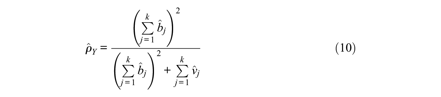
{\hat{ρ}}_{Y} = \frac{{(\sum_{j = 1}^{k} {\hat{b}}_{j})}^{2}}{{(\sum_{j = 1}^{k} {\hat{b}}_{j})}^{2} + \sum_{j = 1}^{k} {\hat{v}}_{j}}

(10)

and

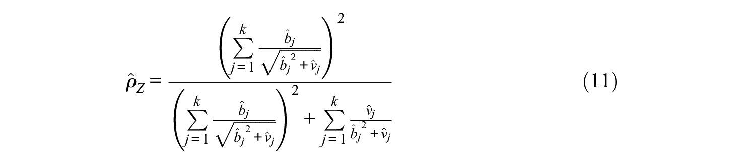
{\hat{ρ}}_{Z} = \frac{{(\sum_{j = 1}^{k} \frac{{\hat{b}}_{j}}{\sqrt{{\hat{b}}_{j}^{2} + {\hat{v}}_{j}}})}^{2}}{{(\sum_{j = 1}^{k} \frac{{\hat{b}}_{j}}{\sqrt{{\hat{b}}_{j}^{2} + {\hat{v}}_{j}}})}^{2} + \sum_{j = 1}^{k} \frac{{\hat{v}}_{j}}{{\hat{b}}_{j}^{2} + {\hat{v}}_{j}}}

(11)

represent the ML estimators of the unstandardized and standardized scale reliability coefficients, respectively, where a hat symbolizes ML estimator (e.g., Bollen, 1989). Then an ML estimator of the population standardized to scale reliability discrepancy, Δ, results as

\hat{Δ} = \frac{{(\sum_{j = 1}^{k} {\hat{b}}_{j})}^{2}}{{(\sum_{j = 1}^{k} {\hat{b}}_{j})}^{2} + \sum_{j = 1}^{k} {\hat{v}}_{j}} - \frac{{(\sum_{j = 1}^{k} \frac{{\hat{b}}_{j}}{\sqrt{{\hat{b}}_{j}^{2} + {\hat{v}}_{j}}})}^{2}}{{(\sum_{j = 1}^{k} \frac{{\hat{b}}_{j}}{\sqrt{{\hat{b}}_{j}^{2} + {\hat{v}}_{j}}})}^{2} + \sum_{j = 1}^{k} \frac{{\hat{v}}_{j}}{{\hat{b}}_{j}^{2} + {\hat{v}}_{j}}} .

Thereby, each of the estimators ${\hat{ρ}}_{Y}$ , ${\hat{ρ}}_{Z}$ , and $\hat{Δ}$ —being ML estimators—possesses highly desirable large sample properties, such as unbiasedness, consistency, normality and efficiency (with respect to the corresponding population scale reliability and standardized reliability coefficients as well as their difference; e.g., Casella & Berger, 2002).

A following subsection demonstrates how a confidence interval at any prespecified confidence level can be obtained for the difference Δ = ρ_Y−ρ_Z of scale reliability and its standardized counterpart. As is well known (e.g., Raykov & Marcoulides, 2008), this interval could also be used for testing (point or simple) null hypotheses about Δ, if need be, in particular that of these two reliability coefficients’ equality, that is, H₀: Δ = 0, or H^*₀: ρ_Y = ρ_Z.

With the preceding discussion in mind, it follows that scale reliability will be equal to its standardized counterpart in the population, that is,

ρ_{Y} = ρ_{Z},

(12)

if and only if

A = B .

(13)

In other words, in those and only those settings when Equation (13) is true, will the standardized reliability be equal to the reliability coefficient of a given scale in a population at large. Similarly, we observe that ρ_Y < ρ_Z, that is, standardized reliability will exceed scale reliability in the population, if and only if A > B. Furthermore, ρ_Y > ρ_Z will hold, that is, standardized reliability will be inferior to scale reliability in the population, if and only if A < B. ²

When Will Standardized Reliability Exceed Scale Reliability?

From Equations (6) through (9) and the earlier discussion in this article, the following conclusion can be made. In all empirical settings where the (population) parameters of the congeneric model (1) are such that the above parametric expression B in Equation (7) is sufficiently smaller than expression A in Equation (9), the standardized reliability ρ_Z will be markedly higher already at the population level than the unstandardized (regular, ordinary, conventional, traditional) scale reliability ρ_Y. Hence, estimating, using, and/or reporting the standardized scale reliability rather than the scale reliability coefficient, can be seriously misleading, especially in the following two aspects. One, the scale in question can be associated then with a reported putative reliability coefficient ( ${\hat{ρ}}_{Z}$ ) that is potentially sufficiently high in order to claim “satisfactory” scale reliability (if ${\hat{ρ}}_{Z}$ is taken at face value, i.e., as the [estimated] index of its reliability). Two, at the same time the actual population scale reliability of real relevance, ρ_Y, can be markedly lower than ρ_Z and possibly deficient—as could be the validity of the scale as well (e.g., McDonald, 1999). We attend next in more detail to this matter.

When Can Standardized Reliability Be Spuriously High?

Examining closely Equations (7) and (9), which define the expressions B and A of ultimate importance for the standardized and scale reliability coefficients, respectively, one can make the following consequential observation. Suppose a scale under consideration is made up of two types of components: (a) some with high reliabilities and (b) some with low reliabilities. If in addition (a) the low reliability components possess each observed variance higher than 1 while (b) the high reliability components exhibit manifest variances smaller than 1, then the contribution of the standardized error variance of the former components to ρ_Z (see Equation 9) will be smaller relative to that of their unstandardized counterparts to ρ_Y (see Equation 7). At the same time, the contribution of the standardized loadings to ρ_Z (see Equation 9) for the more reliable components, will be larger relative to that of their unstandardized counterparts to ρ_Y.³ (Note from Equation 7 that the scale reliability coefficient is an increasing function of any factor loading, but a decreasing function of any error variance, all else being held the same.) In those cases, standardized reliability can markedly exceed scale reliability. In the following illustration section, Example 1 demonstrates this possibility.

When Can Standardized Reliability Be Markedly Inferior to Scale Reliability?

Revisiting Equations (7) and (9), we can arrive at the following “reverse” observation to that made in the previous subsection. Suppose as before that a scale under consideration is made up of two types of components—some with high reliabilities and others with low reliabilities. Let in addition the low reliability components possess observed variances (sufficiently) close to 1, while the high reliability components be associated with manifest variances considerably (sufficiently) higher than 1. Then the contribution of the standardized error variance of the former components to ρ_Z (see Equation 9) will be largely the same as that of their unstandardized counterparts to ρ_Y (see Equation 7). However, the contribution of the standardized loadings to ρ_Z (see Equation 9) for the more reliable components, will be smaller relative to that of their unstandardized counterparts to ρ_Y. In those cases, standardized reliability can be markedly inferior to scale reliability (see also Note 3). In the illustration section that follows, Example 2 demonstrates this possibility.

Evaluating the Population Discrepancy Between Standardized and Unstandardized Reliability

Comparing the right-hand sides of Equations (3) and (6), we notice that the population difference between standardized and scale reliability, Δ = ρ_Y−ρ_Z, is a function of the 2k loadings and error variances associated with the congeneric model (1) (single-factor model). Hence, on fitting this model to data (and finding it plausible), one can use the popular delta method (e.g., Raykov & Marcoulides, 2004) to obtain for any prespecified confidence level a pertinent confidence interval (CI) for the population discrepancy between standardized and scale reliability. This method is implemented for instance in the popular latent variable modeling software Mplus (Muthén & Muthén, 2018) and provides readily the 90%-, 95%, and 99%-CIs of this discrepancy Δ (see also Raykov & Marcoulides, 2011). As indicated earlier in the note, the corresponding of these intervals could be used, if need be, to test (a) the null hypothesis H₀: Δ = 0 stipulating identity of scale reliability and its standardized counterpart (at the .10, .05, or .01 significance levels, respectively), or (b) any other null hypothesis stating this difference Δ as equal instead to another prespecified nonzero value. This confidence interval evaluation procedure is illustrated in the following section.

Large Sample Properties of the Standardized Reliability Coefficient Estimator

From a theoretical and empirical perspective, it is important to also know the behavior of the standardized reliability coefficient estimator in Equation (11) as sample size increases indefinitely (cf. Raykov, 2019). To this end, one can use Theorem 17 in Ferguson (1996, p. 114), from which it follows that under normality the standardized reliability estimator ${\hat{ρ}}_{Z}$ converges with increasing sample size almost surely to the population standardized reliability coefficient, ρ_Z. Hence, based on the preceding discussion, with probability 1 (i.e., almost surely) the standardized reliability estimator ${\hat{ρ}}_{Z}$ (Equation 11) converges then with probability 1 to a quantity that can be markedly higher, or alternatively notably lower, than the population scale reliability coefficient, ρ_Y, which is of actual importance in reliability studies. Given that strong convergence implies also convergence in probability (e.g., Ferguson, 1996), from this almost-sure convergence property it follows that the standardized reliability estimator ${\hat{ρ}}_{Z}$ is then not consistent for the relevant scale reliability coefficient (in particular, it will be inconsistent unless the aforementioned null hypothesis H₀: Δ = 0 is true in the studied population to begin with; see also Note 2). This feature of ${\hat{ρ}}_{Z}$ is in general another serious argument against using standardized reliability as an index informing about a considered scale’s reliability coefficient, $ρ_{Y}$ , of real concern, and is also part of the message of the present article.

Illustration on Data

In this section, we provide a pair of numerical examples of the settings discussed in the previous section, where standardized reliability is markedly higher than unstandardized reliability (Example 1), or alternatively notably inferior to the latter (Example 2). The first is therefore an example where reporting standardized reliability in lieu of scale reliability leaves the wrong impression of unduly high “precision of measurement” with an instrument under consideration. The second example illustrates subsequently the fact that being preoccupied with standardized reliability can be the reason for a scholar to miss a potentially “satisfactory” (“sufficiently high”) level of reliability for a studied scale (version).

Example 1

We use here simulated data on r = 1,000 replications with sample size n = 500 each for a unidimensional scale consisting of k = 4 components, which are generated using the following model:

\begin{matrix} X_{1} = T + E_{1}, \\ X_{2} = . 9 T + E_{2}, \\ X_{3} = . 3 T + E_{3}, \\ X_{4} = . 25 T + E_{4}, \end{matrix}

(14)

where T is standard normal and the error terms E₁ through E₄ are independent normal variates with variances 1.2, 1.2, .03, and .03, respectively. As can be readily seen, and in agreement with the previous section, the first two components, X₁ and X₂, have relatively low reliabilities, namely, in the .40s, but considerably higher observed variances than the last two components, X₃ and X₄; the latter possess thereby relatively high reliabilities—in the .60s and .70s—and notably lower observed variances that are both below 1. The 1,000 replication data sets generated following this model, with sample size n = 500 each, are furnished with the first Mplus command file provided in Appendix B (note the seed employed thereby, for analysis replication purposes). Using Equations (3) and (6), for this setting we obtain through direct algebra the population unstandardized and standardized scale reliability coefficients of ρ_Y = .71 and ρ_Z = .84, respectively. That is, we are dealing here with a four-component measuring instrument that possesses standardized reliability markedly higher—namely, by almost 20%—than the associated scale reliability. Hence, the present is an example where the population standardized scale reliability coefficient is substantially higher (and well above what may be considered a “threshold” for desirable reliability of .80 say), whereas the population unstandardized scale reliability of actual relevance is considerably lower than both its standardized counterpart and such a “threshold.”

When fitting the single-factor model to the 1,000 replication data sets we obtain overwhelmingly tenable overall goodness-of-fit indices that are summarized in Table 1 (following the used software output format; Muthén & Muthén, 2018, chap. 12).

Table 1.

Overall Goodness-of-Fit Statistics of the Single-Factor Model in Example 1 (Mplus Output Format).

Chi-square test of model fit
Degrees of freedom		2
Mean		1.899
Std Dev		1.866
Number of successful computations		1000
Proportions		Percentiles
Expected	Observed	Expected	Observed
0.990	0.991	0.020	0.021
0.980	0.980	0.040	0.039
0.950	0.951	0.103	0.103
0.900	0.903	0.211	0.213
0.800	0.809	0.446	0.481
0.700	0.702	0.713	0.725
0.500	0.484	1.386	1.302
0.300	0.278	2.408	2.232
0.200	0.184	3.219	3.054
0.100	0.087	4.605	4.391
0.050	0.042	5.991	5.697
0.020	0.014	7.824	7.152
0.010	0.008	9.210	8.224
RMSEA (Root Mean Square Error of Approximation)
Mean		0.013
Std Dev		0.022
Number of successful computations		1000
Proportions		Percentiles
Expected	Observed	Expected	Observed
0.990	1.000	−0.037	0.000
0.980	1.000	−0.031	0.000
0.950	1.000	−0.022	0.000
0.900	1.000	−0.015	0.000
0.800	1.000	−0.005	0.000
0.700	0.344	0.002	0.000
0.500	0.313	0.013	0.000
0.300	0.252	0.025	0.015
0.200	0.205	0.032	0.032
0.100	0.138	0.041	0.049
0.050	0.097	0.049	0.061
0.020	0.061	0.058	0.072
0.010	0.039	0.064	0.079

Note. A detailed discussion of the specifics pertaining to the proportions and percentiles reported in this table is provided in Muthén and Muthén (2018, chap. 12).

Table 1 also indicates a fairly good approximation of the theoretical chi-square distribution of the overall goodness-of-fit index by its empirical distribution across the 1,000 replications. The summary fit statistics in it further demonstrate plausible fit for the overwhelming majority of replications (see also Note 4). We then examine the pertinent 1,000 unstandardized and 1,000 standardized scale reliability estimates associated with these replication data sets. Table 2 presents the summary statistics for these 2,000 estimates in total, including in particular the minimal and maximal estimate of standardized reliability and of scale reliability across the 1,000 replications.

Table 2.

Summary Statistics for the Scale Reliability and Standardized Reliability Estimates Across the Simulated 1000 Replication Data Sets in Example 1 (Stata Format).

Variable \|	Obs	Mean	Std. Dev.	Min	Max
unst_rel \|	1,000	.7086757	.0221855	.6442332	.7646031
std_rel \|	1,000	.8391695	.0114685	.7964658	.8681082

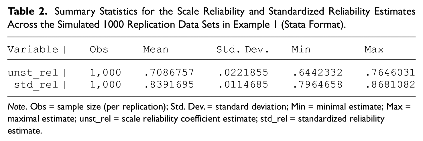
Note. Obs = sample size (per replication); Std. Dev. = standard deviation; Min = minimal estimate; Max = maximal estimate; unst_rel = scale reliability coefficient estimate; std_rel = standardized reliability estimate.

As seen from Table 2 all 1,000 standardized reliability estimates, with a mean of .84 and standard deviation .01, are above the population scale reliability coefficient of .71. That is, 100% of the standardized scale reliability estimates are overestimating—and many times markedly so—the population scale reliability coefficient. Similarly, all scale reliability estimates, with a mean of .71 and standard deviation of .02, are entirely below the population standardized reliability coefficient of .84. In other words, the population standardized reliability coefficient notably exceeds 100% of the scale reliability estimates (as well as its unstandardized scale reliability counterpart). Thereby, even the minimal standardized reliability estimate is considerably higher than the maximal (highest) scale reliability estimate (not necessarily from the same sample). This Example 1 is therefore a clear demonstration of how misleading estimation, reporting, and interpretation of standardized reliability could be if treated as an index of “precision of estimation” for a scale under consideration, as found at times in the empirical literature.^4,5

To illustrate the earlier outlined procedure for evaluation of the scale reliability to standardized reliability discrepancy Δ, we generate a single data set at the same sample size n = 500 with the above model in Equations (14). (In empirical research the typical situation a scholar is in, is when he or she has access only to a single random sample from a studied population.) To this end, we utilize the correspondingly slightly modified first Mplus command file in Appendix B, employing the seed 2296616 say (for details, see Note 2 to that command file). The congeneric test model (1) is found to be associated with tenable fit indices when fitted to the resulting data set: chi-square = 0.099, degrees of freedom = 2, p = .952, and root mean square error of approximation (RMSEA) = 0 with associated 90% CI being (0, 0). In order to evaluate the standardized to scale reliability discrepancy Δ, we use next the third Mplus command file in Appendix B, which furnishes a 95% CI for Δ as (−.14, −.10). Hence, a range of practically highly plausible values for this population difference of scale reliability to standardized reliability stretches from −.14 to −.10. This CI covers the population discrepancy Δ = .71 − .84 = −.13 that we have found above with the known parameters of model (Equations 14) used to generate the analyzed data set. Since this interval does not include 0, if one were to be interested to begin with testing whether scale reliability equals standardized reliability (say at the usual .05 significance level), it would be suggested that the null hypothesis H₀: ρ_Y = ρ_Z can be rejected.

Example 2

Similarly to Example 1, here we simulate data on r = 1,000 replications with sample size n = 500 each for a unidimensional scale consisting of k = 4 components, which are however generated using the following model:

\begin{matrix} X_{1} = . 3 T + E_{1}, \\ X_{2} = . 3 T + E_{2}, \\ X_{3} = 2 T + E_{3}, \\ X_{4} = 2 T + E_{4}, \end{matrix}

(15)

where T is standard normal and the error terms are independent normal variates with variances .5, .5, .8, and .8, respectively. Unlike Example 1 though, in this setting the lower reliability components have observed variances relatively close to 1 but the higher reliability components exhibit variances notably larger than 1. The population standardized and scale reliability coefficients are readily obtained here, with direct algebra using Equations (3) and (6), as ρ_Z = .77 and ρ_Y = .89, respectively. This is therefore an example with markedly inferior standardized reliability already at the population level, since Δ = .89 − .77 = 12. (See the second Mplus command file in Appendix B for the generation of the 1,000 replication data sets, which contains also the seed employed thereby.)

Fitting the single-factor model to the resulting 1,000 data sets shows also overwhelmingly tenable overall fit indices, indicating plausible fit in the large majority of replications (see Table 3).

Table 3.

Overall Goodness-of-Fit Statistics of the Single-Factor Model in Example 2 (Mplus Output Format).

Chi-square test of model fit
Degrees of freedom		2
Mean		1.978
Std Dev		1.987
Number of successful computations		1000
Proportions		Percentiles
Expected	Observed	Expected	Observed
0.990	0.991	0.020	0.024
0.980	0.984	0.040	0.047
0.950	0.950	0.103	0.103
0.900	0.891	0.211	0.200
0.800	0.767	0.446	0.366
0.700	0.675	0.713	0.639
0.500	0.501	1.386	1.386
0.300	0.297	2.408	2.384
0.200	0.204	3.219	3.256
0.100	0.099	4.605	4.594
0.050	0.048	5.991	5.931
0.020	0.016	7.824	7.081
0.010	0.010	9.210	9.095

RMSEA (root mean square error of approximation)
Mean		0.015
Std Dev		0.023
Number of successful computations		1000
Proportions		Percentiles
Expected	Observed	Expected	Observed
0.990	1.000	−0.038	0.000
0.980	1.000	−0.032	0.000
0.950	1.000	−0.023	0.000
0.900	1.000	−0.015	0.000
0.800	1.000	−0.005	0.000
0.700	0.368	0.003	0.000
0.500	0.329	0.015	0.000
0.300	0.261	0.027	0.020
0.200	0.213	0.034	0.035
0.100	0.144	0.044	0.051
0.050	0.095	0.052	0.063
0.020	0.055	0.061	0.071
0.010	0.033	0.068	0.084

Note. A detailed discussion of the specifics pertaining to the proportions and percentiles reported in this table is provided in Muthén and Muthén (2018, chap. 12).

We next examine the resulting 1,000 unstandardized and 1,000 standardized scale reliability estimates across all replications. Table 4 presents the summary statistics for these 2,000 estimates in total, including the minimal and maximal estimates of standardized reliability and of scale reliability.

Table 4.

Summary Statistics for the Scale Reliability and Standardized Reliability Estimates Across the Simulated 1,000 Replication Data Sets in Example 2 (Stata Format).

Variable \|	Obs	Mean	Std. Dev.	Min	Max
unst_rel \|	1,000	.8907072	.0081922	.8595549	.9135987
std_rel \|	1,000	.7700642	.0132522	.7193512	.8055871

We observe from Table 4 that all 1,000 standardized reliability estimates, with a mean of .77 and standard deviation .01, are below the population scale reliability coefficient of .89. That is, 100% of the standardized reliability estimates are underestimating—and many times markedly so—the population scale reliability coefficient. Similarly, all scale reliability estimates, with a mean of .89 and standard deviation of .01, are entirely above the population standardized reliability coefficient of .77. In other words, the population standardized reliability coefficient is notably inferior to 100% of the scale reliability estimates (in addition to being so to the population unstandardized scale reliability coefficient). Thereby, even the minimal scale reliability estimate is considerably higher than the maximal standardized reliability estimate (not necessarily from the same sample).⁶

The present Example 2 is thus an “alternative” demonstration of how misleading estimation, reporting, and interpretation of standardized reliability could be if treated as an index of “precision of estimation” for a considered multicomponent measuring instrument (version). Specifically, in doing so a scholar who is solely preoccupied with standardized reliability may miss a “sufficiently reliable” scale, while treating it as deficient in that respect, as a consequence of this marked underestimation feature of standardized reliability.

Conclusion

The aim of this note was to draw attention to the fact that the standardized reliability coefficient can be seriously misleading empirical behavioral, social, clinical, educational, marketing, and business researchers using it in lieu of—or even in addition to—the regular, (conventional, traditional, “standard,” or ordinary) scale reliability coefficient that is of actual relevance in reliability studies (see Equation 3). Based on the developments in this article, it is recommended that empirical scientists generally refrain from using, estimating, or reporting/ interpreting standardized reliability coefficients of homogenous multicomponent measuring instruments. While this article considered exclusively unidimensional scales (with uncorrelated errors), it may be conjectured that similar findings could be obtained with general structure instruments (cf. Raykov & Shrout, 2002), with their discussion being beyond its confines.

Several limitations of the discussion in this article are worth pointing out here. One is that the note does not imply and is not meant to suggest that in all empirical settings (with unidimensional scales possessing uncorrelated errors) the extent of estimation bias in the standardized reliability coefficients will be similar to that observed in the examples in the “Illustration on Data” section (see also Note 1). We do not exclude therefore the possibility that under certain (potentially fairly restrictive) circumstances this bias may be substantially smaller or even negligible. (An application of the interval estimation procedure for the standardized reliability to scale reliability discrepancy could be helpful in general, as could possibly be testing for their identity, if of interest.) Two, the article does not identify a simple condition that the congeneric test (single-factor) model parameters need to fulfil, in order for the standardized reliability estimation bias to be serious in an empirical setting (cf. Notes 2 and 3). Three, as indicated above, this note assumed throughout that the single-factor model with uncorrelated errors was plausible, and this could also be considered a limitation with respect to possible generalization of its findings to a wider set of empirical settings and studies. Last but not least, the specific conclusions about the population discrepancy Δ between scale and standardized reliability depend strictly speaking on the assumption of (approximately) continuous scale components, and it is thus unknown at present to what extent they may be generalized to discrete component cases.

In conclusion, this article points out a potentially serious drawback of the standardized reliability coefficient that makes it less applicable in empirical research, and in fact potentially seriously misleading, than seems to be the case in some of the substantive behavioral and social science literature of the past several decades.

Footnotes

Appendix A

Appendix B

Acknowledgements

We are grateful to S. Penev, S. Reise, A. Maydue-Olivares, and V. Savalei for valuable discussions on reliability estimation; and to B. Muthén, T. Asparouhov, C. DiStefano, and D. Shi for instructive simulation and software implementation advice.

Declaration of Conflicting Interests

The author(s) declared no potential conflicts of interest with respect to the research, authorship, and/or publication of this article.

Funding

The author(s) received no financial support for the research, authorship, and/or publication of this article.

Notes

References

Apostol

(2013). Calculus. Wiley.

Bentler

P. M.

Satorra

(2010). Testing model nesting and equivalence. Psychological Methods, 15(2), 111-123. https://doi.org/10.1037/a0019625

Bollen

K. A.

(1989). Structural equations with latent variables. Wiley. https://doi.org/10.1002/9781118619179

Casella

Berger

(2002). Statistical inference. Wadsworth.

Ferguson

T. S.

(1996). A course in large sample theory. Chapman & Hall. https://doi.org/10.1007/978-1-4899-4549-5

Jöreskog

K. G.

(1971). Statistical analysis of sets of congeneric tests. Psychometrika, 36(2), 109-133. https://doi.org/10.1007/BF02291393

Jöreskog

K. G.

Sörbom

(1996). LISREL 8 user’s guide. Scientific Software.

McDonald

R. P.

(1999). Test theory. A unified treatment. Lawrence Erlbaum.

McNeish

(2018). Thanks coefficient alpha, we’ll take it from here. Psychological Methods, 23(3), 412-433. https://doi.org/10.1037/met0000144

10.

Muthén

L. K.

Muthén

B. O.

(2018). Mplus user’s guide. Muthén & Muthén.

11.

Raykov

(2012). Scale development using structural equation modeling. In Hoyle

(Ed.), Handbook of structural equation modeling (pp. 472-492). Guilford Press.

12.

Raykov

(2019). Strong consistency of reliability estimators for multiple-component measuring instruments. Structural Equation Modeling, 26(5), 750-756. https://doi.org/10.1080/10705511.2018.1559737

13.

Raykov

Marcoulides

G. A.

(2004). Using the delta method for approximate interval estimation of parametric functions in covariance structure models. Structural Equation Modeling, 11(4), 659-675. https://doi.org/10.1207/s15328007sem1104_7

14.

Raykov

Marcoulides

G. A.

(2008). An introduction to applied multivariate analysis. Taylor & Francis. https://doi.org/10.4324/9780203809532

15.

Raykov

Marcoulides

G. A.

(2011). Introduction to psychometric theory. Taylor & Francis. https://doi.org/10.4324/9780203841624

16.

Raykov

Marcoulides

G. A.

(2019). Thanks coefficient alpha, we still need you! Educational and Psychological Measurement, 79(1), 200-210. https://doi.org/10.1177/0013164417725127

17.

Raykov

Marcoulides

G. A.

Chang

(2016). Studying population heterogeneity in finite mixture settings using latent variable modeling. Structural Equation Modeling, 23(5), 726-730. https://doi.org/10.1080/10705511.2015.1103193

18.

Raykov

Shrout

(2002). Reliability of scales with general structure: Point and interval estimation using a structural equation modeling approach. Structural Equation Modeling, 9(2), 195-212. https://doi.org/10.1207/S15328007SEM0902_3

19.

Zimmerman

D. W.

(1975). Probability spaces, Hilbert spaces, and the axioms of test theory. Psychometrika, 40(3), 395-412. https://doi.org/10.1007/BF02291765