
Abstract
The purpose of this two-part study is to evaluate methods for multiple group analysis when the comparison group is at the within level with multilevel data, using a multilevel factor mixture model (ML FMM) and a multilevel multiple-indicators multiple-causes (ML MIMIC) model. The performance of these methods was evaluated integrally by a series of procedures testing weak and strong invariance models and the latent group mean differences testing after holding for factorial invariance. Two Monte Carlo simulation studies were conducted under the following conditions: number of clusters, cluster size, and the design type in groups. A multilevel one-factor confirmatory factor analysis (CFA) model as a research model in Study 1 was investigated to compare the results under different conditions with those of previous studies. A multilevel two-factor CFA model as a research model in Study 2 was evaluated by fitting alternative models that can be applied when the model is complicated. The results indicated that the two methods were reasonable in multilevel multiple groups analysis across within-level groups. However, pros and cons were found between the two methods. In the multilevel one-factor CFA model, ML MIMIC model was slightly better when the sample size is small. In the multilevel complex model, two alternative models of ML FMM were recommended because the weak invariance testing of ML MIMIC was considerably time-consuming. Finally, it was shown that information criteria, which are criteria for determining whether factorial invariance is established, need to be applied differently according to the sample size conditions. Guidelines for this situation are provided.
Keywords
Introduction
Multiple group analysis is used to test whether the parameters of interest are statistically different across comparison groups. In the social and behavioral sciences, a number of studies address the methodology of multiple group analysis (e.g., Cheung & Rensvold, 1998; Kim et al., 2017; Morin et al., 2016; Vandenberg & Lance, 2000). Recently, with the popularity of multilevel data (e.g., when individuals are nested within organizations, when students are nested within classes or schools, etc.), several issues regarding multiple group analysis in multilevel structural equation modeling (MSEM) are worthy of attention. A group is distinguished from clusters and refers to the memberships to be compared.
When multiple group analysis is studied with multilevel data, comparing groups can be either at within level (e.g., male students vs. female students) or at between level (e.g., public schools vs. private schools). If the grouping variable is at the between level, all the individuals in each cluster belong only to a single group, whereas if the grouping variable is at the within level, each cluster may have several groups (Asparouhov & Muthén, 2012b; Kim & Cao, 2015; Kim et al., 2015; Ryu, 2014). For example, when comparing gender differences using data of students nested within schools, there are males and females in coeducational schools. Between-level grouping analysis is relatively easier than within-level grouping analysis because it can be solved in a standard way as in single-level multiple group analysis. The standard procedure of a multiple group approach is that a set of data is first split by groups and the same model is specified in each group (i.e., configural invariance). Then the models are simultaneously estimated with the equality constraints (i.e., factor loading and intercept invariance). It should be noted that an important assumption of the multiple group analysis is an independent assumption where individuals are randomly extracted from the population. Between-level grouping variable analysis can be regarded as satisfying this assumption. However, within-level grouping analysis raises a complex problem because within-level groups are generally not independent. As these gender groups share a common variable at the between level (e.g., school environment, teacher’s teaching quality), the data cannot support the independence assumption and also cannot be completely separated. Hence, a key issue with using multiple group analysis across within-level groups is a question of how to consider the dependency at the between level. Despite the increasing number of studies on multilevel data, the methodology of multilevel multiple group analysis has not been sufficiently studied, and group comparison studies have not been actively conducted in the social sciences such as education and psychology.
To address this problem, a few recent studies proposed some approaches and investigated the performance of each method: (1) multilevel factor mixture model (ML FMM) as a multiple group approach (Asparouhov & Muthén, 2012b) and (2) multilevel multiple-indicators multiple-causes (ML MIMIC) model as a single group approach (Kim et al., 2015; Woods & Grimm, 2011).
This study builds on recent findings that ML FMM and ML MIMIC are appropriate for within-level factorial invariance testing and latent group mean comparison (Kim & Cao, 2015; Kim et al., 2015). By expanding on the contributions of previous studies, this study differs in the following aspects. First, given that factor invariance testing is a prerequisite for multiple group analysis, integrated guidelines for factor invariance testing procedures and latent group mean difference testing should be suggested. Previous studies carry limitations in that they are evaluating the performance of methods for two types of testing (i.e., factorial invariance testing, latent group means difference testing) in separate studies. Although researchers may be interested only in the establishment of factorial invariance, generally it is accompanied by factorial invariance testing and the comparison of latent means. Moreover, it is insufficient to conduct only the latent mean comparison, without testing factorial invariance. Second, since it is a methodology aimed at comparing two groups, it is necessary to pay particular attention to whether performance is sensitive to unbalanced sample sizes between the two groups. However, previous studies investigating the performance of both methods have considered various sample sizes of a number of clusters and cluster size as a condition but have not considered whether the two groups were balanced. To fill this gap, this study compared the performances of two methods by focusing on sample size conditions including design type (balanced or unbalanced) as well as the number of clusters and cluster size. Last, for complex models with two or more factors or with three or more comparison groups, the performance of the two methods needs to be considered. The complex model in this study refers to cases where the number of factors increases (i.e., multilevel multiple-factor model) or the number of groups increases (i.e., comparisons of more than two groups). The basic models of ML FMM and ML MIMIC, which were applied in a multilevel one-factor confirmatory factor analysis (CFA) model, are not applicable to complex models. The reason is technically related to the estimation method. To estimate group-specific random effects at the between level, the estimation of ML FMM uses numerical integration and the dimensions are required for as many G groups per factor (i.e., number of dimensions = number of factors × number of groups; Asparouhov & Muthén, 2012b). Hence, when conducting multiple group analysis using ML FMM, a multilevel one-factor CFA model and a multilevel two-factor CFA model require two and four dimensions, respectively. However, analysis of a complex model is likely to lead to estimation problems. In fact, it is impossible to estimate two more dimensions in current software programs, including Mplus. Besides ML FMM, ML MIMIC also has difficulty in estimation in the case of a complex model. One of the disadvantages of the MIMIC approach is that it is not easy to implement weak invariance testing because it also requires numerical integration due to latent interaction terms (i.e., interaction between a factor and grouping variable). Hence when the model has more than one factor, it needs as many latent interaction terms as the number of factors in weak invariance testing, which requires a considerable amount of time. Therefore, to analyze a complex model, alternative methods are needed. To seek a solution, this study addresses modeling issues for a complex model in multiple group analysis and reviewed alternative models proposed by Asparouhov and Muthén (2012b). Alternative models in this study are more restricted models in which group specific random effects are set proportionally or equalized between two groups (see “Theoretical Background” section for more details). By evaluating the performances of the alternative models, this study offers suggestions in terms of to what extent the complex model can be generalized.
The purpose of this study is to provide practical guidelines for which method is appropriate, ML FMM and ML MIMIC, when multilevel multiple group analysis is conducted with a within-level grouping variable. To achieve this objective, this study explicated the factorial invariance testing procedures of two methods (ML FMM and ML MIMIC) and elucidated a model specification about a complex model (i.e., multiple-factor model or more than two groups analysis). Two simulation studies were conducted to investigate the efficacy and performances of the two methods: a multilevel one-factor CFA model in Study 1 and a multilevel two-factor CFA model as a complex model in Study 2. Study 1 confirmed that the same result was obtained from the previous study under different sample size conditions including unbalanced design types. In Study 2, alternative methods were suggested, and the performance of those was examined. In addition, this study also tried to generalize alternative models to the more complex models (e.g., three-factor model or three groups comparison). Last, this study provides a practical guideline for applied researchers.
The current study will address the following research questions:
Theoretical Background
Multiple Group Analysis
The establishment of factorial invariance allows for the interpretation of a latent construct in the same manner between groups; thus, factorial invariance testing is a prerequisite to compare observed scores or latent factor means across groups (Mellenbergh, 1989; Meredith, 1993; Meredith & Millsap, 1992; Millsap, 1997; Reise et al., 1993). Factorial invariance testing generally requires four sequential procedures: configural, weak, strong, and strict invariance. Configural invariance refers to having equivalent patterns (i.e., zero and nonzero patterns) of factor structure across groups (i.e., the same number of factors and indicators across groups). Weak invariance (also referred to as metric or factor loading invariance) requires equal factor loading between groups in addition to configural invariance. Strong invariance (also referred to as scalar or intercept invariance) holds invariant measurement of intercepts in addition to weak invariance between groups. Strict invariance indicates invariant measurement of residual variance in addition to equal factor loading and intercepts. According to the literature on factorial invariance, it is known that a strong invariance model should be established for a statistically reasonable group mean comparison (Jak et al., 2014; Widaman & Reise, 1997). That is, strict invariance testing is not considered essential when testing latent mean differences between groups. The establishments of weak and strong invariance are particularly important in factorial invariance testing. Accordingly, the establishment of configural invariance was assumed in this study, and only the performances of weak and strong invariance testing were assessed. Also, this study did not examine the performance of strict invariance testing.
Multilevel Factor Mixture Model for Known Classes
Factor mixture modeling (FMM) is a combined model of traditional CFA and latent class analysis that incorporates latent continuous variables (i.e., factors) and latent categorical variables (i.e., latent classes; Asparouhov & Muthén, 2008; Lubke & Muthén, 2005). In general, FMM is used as an analytical method to identify heterogeneous populations in the data and to derive latent classes. In a multiple group analysis framework, FMM also can be employed for factorial invariance testing and latent mean difference testing across groups in which observed groups are treated as known classes.
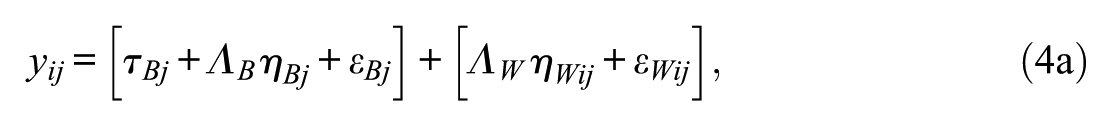
In ML FMM across within-level groups, the group effects are estimated as random effects at the between level. ML FMM for within-level groups is specified as (Asparouhov & Muthén, 2012b; Kim & Cao, 2015)
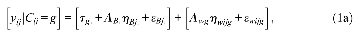
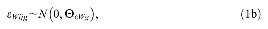
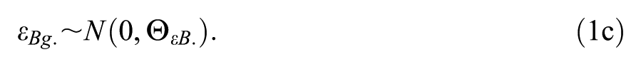
where a subscript

In ML FMM, group-specific random effects are specified by the latent variable (i.e., e1 for males and e2 for females), and these random effects are correlated, representing the dependency. For each group, e1 and e2 are specified to have zero residual variance and perfectly related to the corresponding between-level factors. The variance of e1, e2, and the correlation (or covariance) between e1 and e2 (called intraclass group correlation coefficient [IGCC] in Kim and Cao’s, 2015, article) are estimated freely in the model.
Importantly, ML FMM in multiple group analysis uses numerical integration for model estimation. Hence, the estimation problem may occur when the model is complex as in the case of a CFA model with more than one factor (i.e., multidimensional constructs) or more than two groups (e.g., comparison of school levels: elementary, middle, and high school) due to an increased dimension in numerical integration. Accordingly, Asparouhov and Muthén (2012b) suggested six alternative models since a parsimonious model that is more restricted but easier to estimate may be appropriate depending on the data. Among these models, there are two alternative models that are suitable for the testing of factorial invariance and latent mean difference. Other models can easily be applied to the estimation of the latent mean differences, but it is almost impossible to test for factorial invariance (for more details, see Asparouhov & Muthén, 2012b).
The first alternative model (referred to as the ML FMM A1 model hereinafter in this study) is a slightly restricted model and nested in the ML FMM described above. While general ML FMM in multiple group analysis has separate group-specific random effects between groups, ML FMM A1 has different group-specific random effects but assumes to have a perfect correlation between these effects (i.e., the correlation = 1), indicating that the group-specific random effects have a proportional relationship. The variance of random effects is fixed to 1 and different group-specific variances across groups are represented by the freely estimated factor loadings for the random effect. Since it is expected to have highly correlated cluster effects in many educational and psychological applications, this assumption may be reasonable (Asparouhov & Muthén, 2012b; Ryu, 2014; Ryu & Mehta, 2017).
The second alternative model (referred to as the ML FMM A2 model hereinafter in this study) is a more restricted model than ML FMM A1 and also nested in the ML FMM A1. ML FMM A2 is assumed to have a common set of between levels across groups. That is, ML FMM A2 has an equal variance of cluster-specific effects (i.e., the variance is equally constrained) in addition to the correlation of 1 between group-specific effects; thus, the group effect is estimated as a fixed effect. (i.e., exactly the same between-level model). In this model, there is no need for a random effects variable for the between model.
Factorial Invariance Testing Procedure
In a multilevel multiple group approach, factorial invariance should be established not only across groups but also across the within and between levels (Jak, 2018; Jak & Jorgensen, 2017; Ryu & Mehta, 2017). In Ryu and Mehta’s (2017) article, this was called metric invariance across levels. Although multilevel modeling has flexibility in that the model can be specified differently at each level, it requires the same factor structure across the levels in multiple group analysis (Kim et al., 2012; Ryu & Mehta, 2017). With metric invariance across levels, the total variance of a factor can be divided into within and between levels (Zyphur et al., 2008). In addition, latent factors can represent the same construct conceptually at both levels (e.g., self-efficacy of students at the within level represent average self-efficacy of a school at the between level), which enables them to be labeled in the same way. With this outcome, a latent group mean occurring within level can be estimated at a between level (Asparouhov & Muthén, 2012b).
With metric invariance across levels, Equation (1a) is simplified to
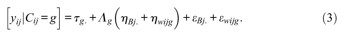
Now the procedure of factorial invariance for ML FMM is similar to multiple group analysis of single-level data. The holding for weak invariance was assessed by model comparison testing between a factor loading equally constrained model across the groups (i.e., weak invariance model,
Strengths and Weaknesses
ML FMM is considered the most general and flexible model in that the dependency between group effects can freely be estimated depending on the modeling. The dependency across groups in the same cluster can be represented by separate sets of group-specific random effects at the between level with the freely estimated as their correlation. Or it can be estimated as a constrained model to reduce the number of parameters. There can be two models in which the correlation is assumed to be 1. One is the group-specific random effects 1 having proportional effects across groups (referred to as ML FMM A1 in this study); the other is the same cluster effects across groups (referred to as ML FMM A2 in this study). Although it is not often seen, the correlation between groups can be assumed to be zero.
Obviously, high power and properly controlled Type I errors are expected in the group-specific random effects model with the freely estimated as their correlation. However, estimation of this model involves a burden on large sample size. In small sample size data, there will not be enough power to establish statistical significance for the group-specific effects. In addition, when the group-specific random effects and IGCC were incorrectly constrained differently from the data, a high Type I error rate and low statistical power resulted (Kim & Cao, 2015).
On the other hand, multiple group analysis in the ML FMM is not possible when the factor structure across levels is different because the mean parameters (i.e., latent factor means, intercepts) are specified at the between level under the assumption that the latent factors have equal meanings at different levels (i.e., metric invariance across levels).
Multilevel Multiple-Indicators Multiple-Causes Model
MIMIC modeling is generally used to test factorial invariance and group mean differences in latent variables (Jöreskog & Goldberger, 1975; Muthén, 1989). Unlike the multiple group analysis approach, MIMIC employs a dummy-coded grouping variable as a covariate to test factorial invariance. The MIMIC model can be extended to an ML MIMIC modeling in hierarchically structured data. When there are groups at the within level, a grouping covariate (
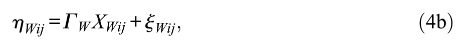
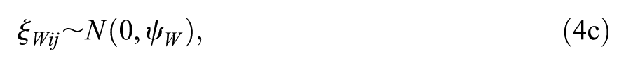
where
Factorial Invariance Testing Procedures
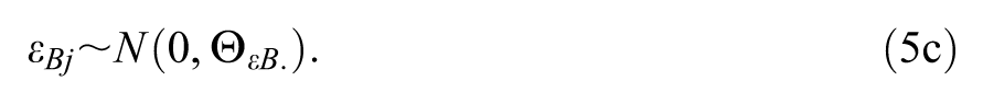
In the MIMIC modeling, sequential invariance testing (i.e., configural, weak, and strong invariance testing) is examined with the significance of the corresponding regression coefficient (Mellenbergh, 1989). Equations (5a) to (5c) specify the configural invariance model, which may differ in intercepts and factor loading between groups.

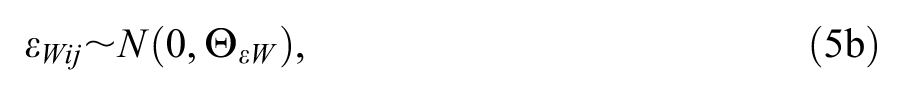
Specifically, the grouping variable (
Strengths and Weaknesses
ML MIMIC has a smaller number of parameters to be estimated than ML FMM because it uses the whole sample to estimate the group difference instead of dividing the data by groups, which ensures adequate power for relatively small samples (Woods, 2009). Another benefit to multiple group analysis using this model is that the model can easily incorporate additional variables (e.g., socioeconomic status, disposition, motivation) that can potentially explain group differences. Despite its advantages, ML MIMIC has a few downsides. Although the factor variance and residual variance of observed variables may be different across groups, MIMIC modeling assumes homogeneity regardless of the number of groups (i.e., stringent assumption). In addition, when multiple group analysis is conducted with within-level groups, group-specific effects cannot be estimated as a random effect, which does not allow for the estimation of the correlation (or covariation) between within-level groups. Importantly, weak invariance testing entails a technical and time-consuming burden. As described above, weak invariance testing in MIMIC involves an interaction term with factors. Unlike interaction terms between observed variables, interaction terms with factors require numerical integration for analysis. As the number of factors increases, the dimension of numerical integration increases, making it almost impossible to estimate. Therefore, the weak invariance test in the two-factor model in Study 2 was conducted by fitting the model of each interaction term with a factor instead of creating two interaction terms with factors at one time.
Previous Simulation Studies
To evaluate the performance of methods of multilevel multiple group analysis when the grouping variable is at a within level, there have been several recently conducted simulation studies. A summary of prior simulation studies is presented in Table 1. 2 Kim et al. (2012) utilized the design-based multiple group multilevel CFA (i.e., single-level approach) to account for the dependency at the between level across the within-level groups. This method takes into account the hierarchical data structure by adjusting standard errors of the parameter estimates using the Type = COMPLEX routine in Mplus. Although this method showed desirable performance in terms of an admissible solution rate, statistical power, and Type I error, it raises questions about group-specific effects across within-level groups not considered in the data generation. That is, an ideal and special situation was assumed.
Summary of Previous Simulation Studies.
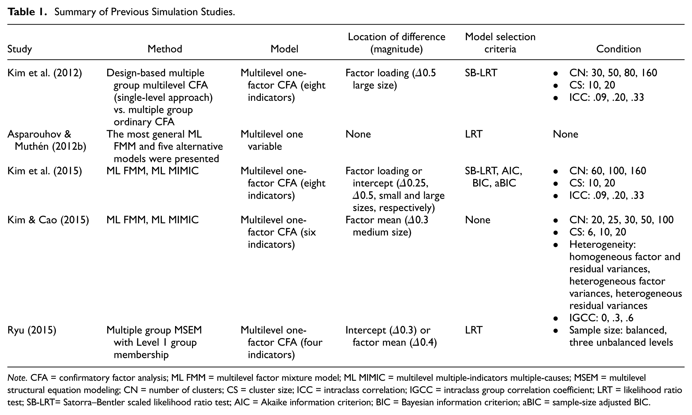
Note. CFA = confirmatory factor analysis; ML FMM = multilevel factor mixture model; ML MIMIC = multilevel multiple-indicators multiple-causes; MSEM = multilevel structural equation modeling; CN = number of clusters; CS = cluster size; ICC = intraclass correlation; IGCC = intraclass group correlation coefficient; LRT = likelihood ratio test; SB-LRT= Satorra–Bentler scaled likelihood ratio test; AIC = Akaike information criterion; BIC = Bayesian information criterion; aBIC = sample-size adjusted BIC.
Asparouhov and Muthén (2012b) presented the Mplus web note for multiple group multilevel analysis. They proposed the ML FMM, which was the most flexible model to estimate group-specific random effects (referred to as model H1 in their article) and suggested five alternative models that were gradually constrained from model H1. Also, a small-scale simulation was conducted to present how the log-likelihood values for the six different models differ from the true model (i.e., model H1). Since they focused on estimating the mean difference between groups, there were models that were not practically able to perform factorial invariance testing among these proposed alternative models.
To examine the performance of factorial invariance, Kim et al. (2015) investigated the adequacy of the ML FMM and ML MIMIC. Additionally, the performance of model selection criteria (Satorra–Bentler scaled likelihood ratio test [SB-LRT], Akaike information criterion [AIC], Bayesian information criterion [BIC], and sample-size adjusted BIC [aBIC]) for determining factorial invariance for ML FMM or in detecting item noninvariance for ML MIMIC was examined. Their study reported that the two approaches were optimal although ML FMM was less optimal when the sample size was as small as 600. However, it should be noted that restricted ML FMM that ignored the group-specific random effects at the between level was investigated.
In addition, Kim and Cao (2015) compared the performance of the two methods (ML FMM and ML MIMIC) for the group mean differences of the latent variable with factorial invariance assumed. The population model was the most general ML FMM, but the MIMIC showed comparable performance to the ML FMM by calculating the average value although the factor and residual variance between the two groups were set differently (i.e., heterogeneity). Additionally, they examined the performances of several different models of ML FMM (i.e., IGCC freely estimated, fixed at zero, fixed at one, and without group-specific random effects) and ML MIMIC with a focus on the specification of the IGCC in another study. In their study, the performance of the model that freely estimates the IGCC was the best, and the model with the IGCC fixed at one had a high power, but Type I errors were substantially inflated regardless of the IGCC conditions. On the contrary, the model without group-specific random effects properly controlled Type I errors, but the power was unacceptably very low. Rather, the model with IGCC fixed at zero indicated a slightly better performance in terms of both evaluation criteria.
Ryu (2014, 2015) suggested multiple group MSEM with Level 1 group membership (referred to as MG1-MSEM in her article) as a multiple group approach. To consider the dependence within the clusters properly, MG1-MSEM first decomposes the variance–covariance matrix into each level components before separating the data by groups. Then, a single-level CFA is set up with an identical between-level model for each group irrespective of their group membership by assuming that the correlation between within-level groups is perfect. MG1-MSEM is available only in Muthén’s maximum likelihood estimation (MUML; Muthén, 1994) and should be manually set up as many 2 *k groups single-level CFA models, where k equals the number of groups. Although MG1-MSEM can be easily applied to more complicated models such as a path model, it is less flexible than ML FMM in that MG1-MSEM only allows a common set of between-level random effects (i.e., correlation = 1) for groups (Ryu & Mehta, 2017).
Method
Simulation Design
To evaluate the performance of ML FMM and ML MIMIC for multiple group analysis in a multilevel CFA model across within-level groups, two Monte Carlo simulations were conducted. As a research model, a multilevel CFA model with one factor (Figure 1) and two factors (Figure 2) were examined in the first and second study, respectively. The model of Study 1 is a multilevel one-factor CFA model similar to previous studies.
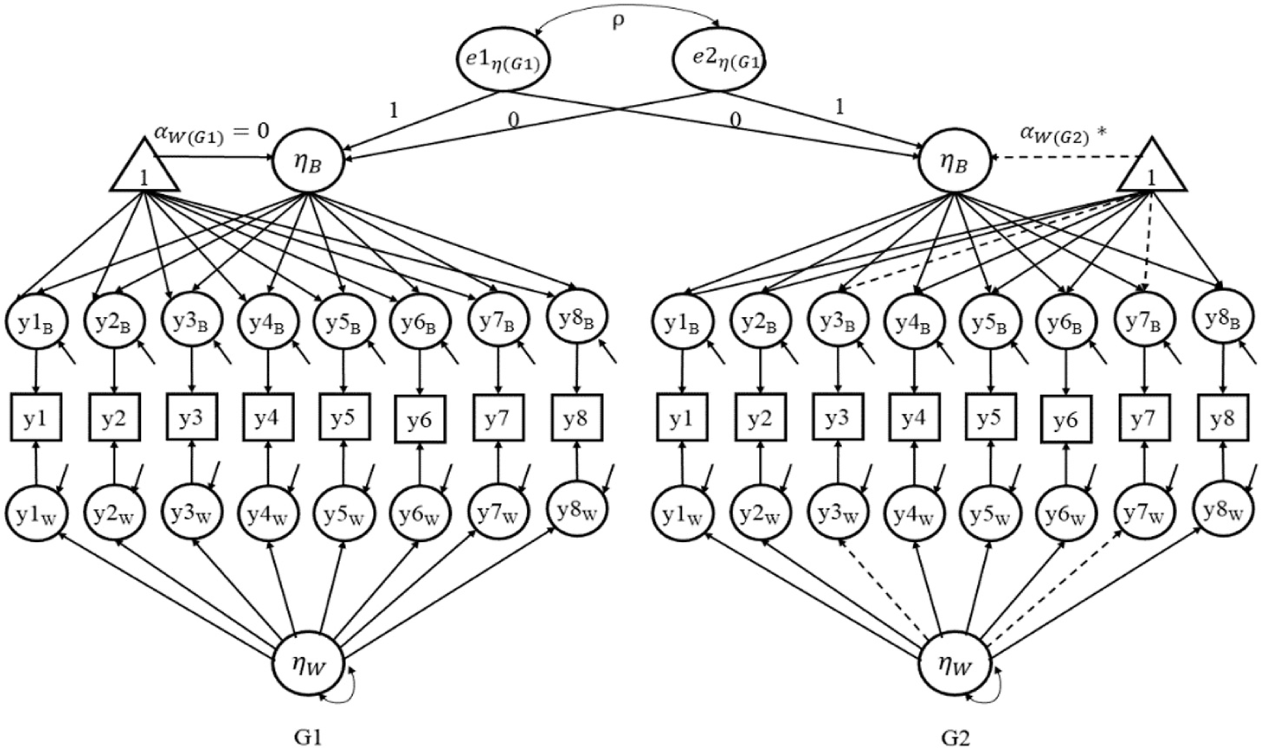
A multilevel confirmatory factor analysis population model of Study 1.

A multilevel confirmatory factor analysis population model of Study 2.
The simulation design is represented in Table 2. The generation model was ML FMM, which is most general and flexible because the group-specific random effects and their correlation are estimated. Four models were generated: two factorial noninvariance models depending on the location of noninvariance (i.e., factor loading or intercept) and two factorial invariance models depending on whether there is a mean difference in the latent variable. The power for the establishment of factorial invariance was calculated by fitting the constrained model (i.e., an unspecified model) and unconstrained model (true model) using the data of the factorial noninvariance model. The power for estimating the latent group mean parameter was calculated using the factorial invariance model with latent group means differences. In addition, a factorial invariance model with zero mean difference was simulated to assess Type I errors.
Simulation Design.
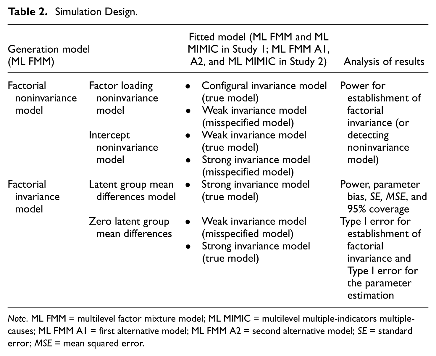
Note. ML FMM = multilevel factor mixture model; ML MIMIC = multilevel multiple-indicators multiple-causes; ML FMM A1 = first alternative model; ML FMM A2 = second alternative model; SE = standard error; MSE = mean squared error.
Simulation Design Factors
Simulation design factors were considered in the two studies: number of clusters (CN), cluster size (CS) and design types in groups (DT). Three different numbers of clusters were simulated (i.e., 30, 50, and 100 per within-level group). Prior simulation studies on multilevel modeling indicated that CN was an important factor in the estimation of the model (Hox & Maas, 2001; Maas & Hox, 2005). In addition, studies on factorial invariance testing with multilevel data reported that CN was positively associated with the power of detecting the noninvariance items and slightly related to the inflation of Type I errors (Kim et al., 2015). The difference of the performance of ML FMM and ML MIMIC was expected to be evident when the CN was small because the two methods have a different number of free parameters that are related to model complexity as reviewed before. In addition, although 100 was considered a minimum number of clusters to obtain stable results (Hox et al., 2010), as in practice, the number of clusters was often much smaller than 100 except for large-scale assessment projects. The cluster sizes of 15 and 30 were chosen based on previous multilevel simulation studies (Hox, 1998; Kim & Cao, 2015; Kim et al., 2012; Kim et al., 2015). The combination of the CN and CS created total sample sizes that ranged from 450 to 3,000. CS was split for each group depending on the design type in the groups because grouping variables occurred at the within level. The groups were designed as balanced or two unbalanced types. The ratio between the two groups was set to 1:1 in a balanced type but 1:2 or 1:3 in the unbalanced types. According to previous studies, sample size in a group that is as small as 20% of the total sample was considered to be at the extreme but statistically estimable sample size (Henson et al., 2007; Tofighi & Enders, 2008). For example, when the cluster size was 15, it was divided into five in the focal group and 10 in the reference group on average in a 1:2 unbalanced type. This means that not divided by an integer of the same size for all replication, on average, two groups were generated at a ratio of 1:2 across 500 replications. In the same way, for these conditions of cluster sizes of 15 or 30 and unbalanced groups of 1:2 or 1:3, on average, 500 replications were generated that met these conditions. The larger sample size served as the reference group.
Data Generation and Analysis
Data Generation
Two-level data with within-level groups (e.g., males and females) were generated. For both within and between levels (i.e., identical factor structure), a single factor with eight indicators and two factors with four indicators were constructed in Study 1 and Study 2, respectively. Two of the eight indicators (
In the noninvariance model, two indicators (i.e., y3 and y7) were set differently. For factor loading noninvariance, all the factor loadings of the first group (i.e., reference group) were .80 except for reference item
To create population heterogeneity, the factor variances across group membership were set differently (e.g., when the group is a balanced design, 1.0 for Group 1 and 1.5 for Group 2 at the within level and 0.1 for Group 1 and 0.2 for Group 2 at the between level). ICC was set to around 0.1. This size is considered small in previous simulation studies (e.g., Hox & Maas, 2001; Jak & Oort, 2015; Kim et al., 2012; Kim et al., 2015; Maas & Hox, 2005) but most commonly seen in educational and psychological studies. The IGCC was set to 0.8. In more general cases, group-specific random effects are expected to be highly correlated in education and psychological contexts (Asparouhov & Muthén, 2012b). According to Ryu and Mehta’s (2017) study, the IGCC of a math self-efficacy latent variable for males and females in PISA 2003 data was .988, which was close to 1. With such high correlation in the educational and psychological context, .8 was considered an appropriate value.
Eighteen conditions (3 CN × 2 CS × 3 DT) per four models (i.e., two noninvariance and two invariance models) that resulted in 72 models were involved in the data generation. For each condition, 500 replications are generated. Models were estimated with maximum likelihood with robust standard errors (MLR), which is known to be robust for nonnormality and nonindependence observations. Data generation and all subsequent analysis were conducted with Mplus 8.3 (Muthén & Muthén, 2015).
Fitted Model
Each replication was analyzed both using ML FMM and ML MIMIC in Study 1 and three times using ML FMM A1, ML FMM A2, and ML MIMIC in Study 2. Two alternative models (i.e., ML FMM A1, ML FMM A2), which were more restricted models, were evaluated due to the convergence problem caused by the increased dimension of numerical integration. In addition, ML MIMIC for a two-factor CFA model entails a different model specification with ML MIMIC for a one-factor CFA model. Importantly, in the testing of the weak invariance model, the interaction term between the factor and the grouping variable should be generated, which means that the number of interaction terms increases by the number of factors. The interaction term between the factor and the observation variable is also required to be estimated using numerical integration, which takes a considerable amount of time to converge. Therefore, the weak invariance testing of ML MIMIC in Study 2 detects noninvariance indicators separately for each factor.
Evaluation Criteria
First, to evaluate the adequacy of the two methods (ML FMM and ML MIMIC), this study investigated the convergence rates. Convergence rates refer to the replications in which the model estimation is computed successfully. On the other hand, nonconvergence means that the solution is not mathematically produced due to a negative variance or a singular matrix.
Second, power and Type I errors were assessed in factorial invariance testing using model selection criteria. Power is defined as the proportion of replications in which the level of noninvariance is correctly detected. That is, power is the proportion at which the configural model (i.e., model with unconstrained factor loading) is selected when the factor loading is noninvariant across the groups. At the same time, power is the proportion at which the weak model (i.e., model with unconstrained intercepts) is selected when the intercept is noninvariant across the groups. In contrast to power, a Type I error is computed as the proportion of replications in which an invariance model is falsely rejected at
In latent mean difference testing, power, Type I errors, bias, mean squared error (MSE), and 95% coverage were assessed. Power here refers to the proportion of replication in which the latent mean difference is detected when the difference truly exists in the population. On the other hand, the Type I error here is computed as the proportion of replications in which zero mean difference between groups was falsely rejected at
Results: Study 1
Convergence Rates
For ML FMM, all replications converged perfectly under many conditions and the lowest rate was 92.8%. However, the convergence rates for ML MIMIC were relatively low from 74.4% to 98.6% and especially for the two unbalanced types. Overall, there were no notable differences in the convergence rate depending on the levels of the factorial invariance testing model (i.e., weak and strong invariance model testing) and across conditions (number of clusters, cluster size, and design types). Even under the worst condition, assumed as a small sample (CN = 30, CS = 15, 1:3 unbalanced group size), both methods showed a high convergence rate (92.8% for ML FMM and 79.8% for ML MIMIC in the weak invariance testing model), indicating high usability in the applied study.
Type I Errors and Power of Factorial Invariance Testing Using Model Selection Criteria
Table 3 present the results of Type I errors and power of factorial invariance testing for ML FMM and ML MIMIC with a multilevel one-factor CFA model using model selection criteria (i.e., SB-LRT, AIC, BIC, and aBIC). Also, the performances by model selection criteria are presented in Figure 3 for specific conditions.
Type I error and Power of Factorial Invariance Testing in Study 1.
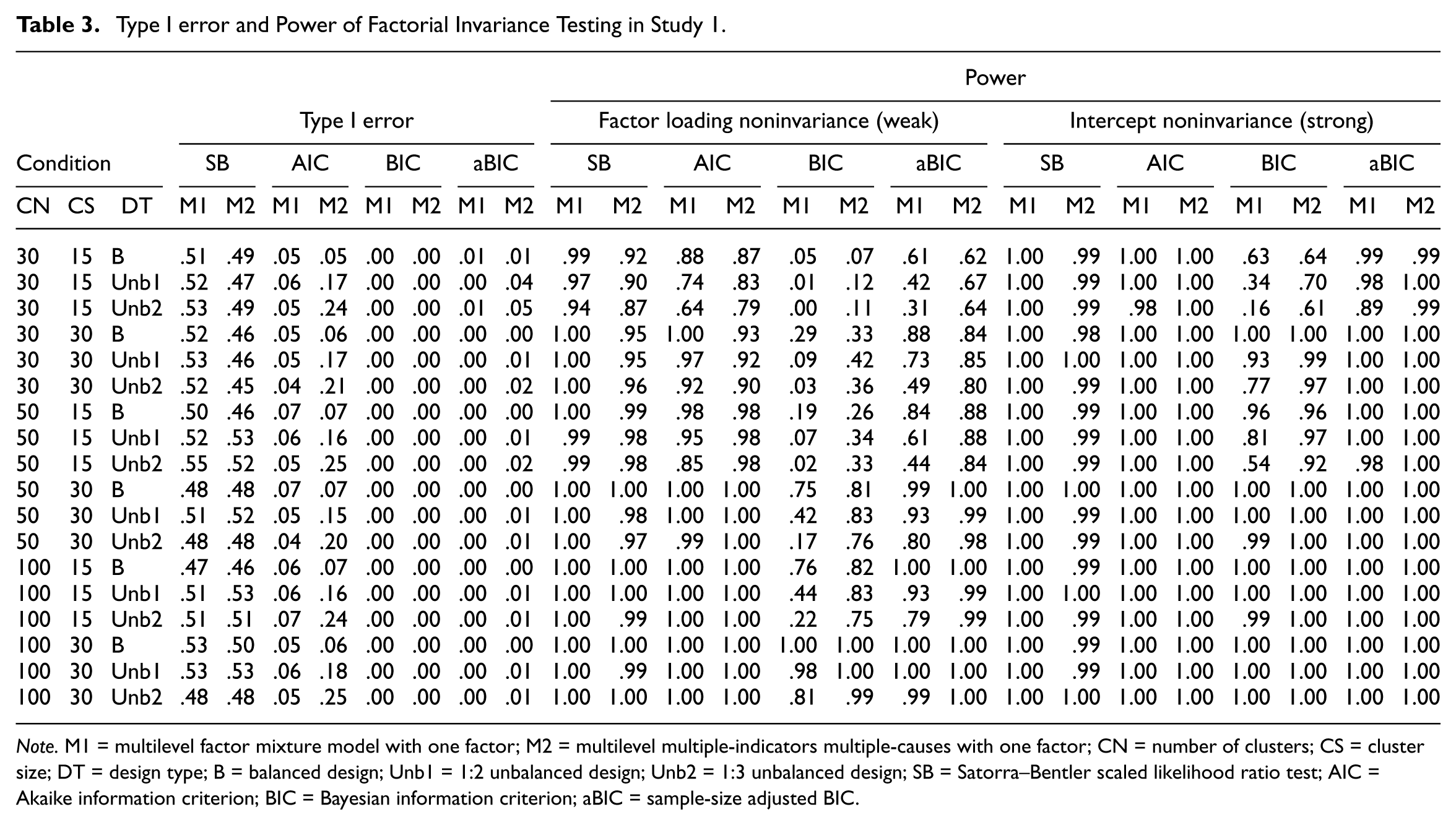
Note. M1 = multilevel factor mixture model with one factor; M2 = multilevel multiple-indicators multiple-causes with one factor; CN = number of clusters; CS = cluster size; DT = design type; B = balanced design; Unb1 = 1:2 unbalanced design; Unb2 = 1:3 unbalanced design; SB = Satorra–Bentler scaled likelihood ratio test; AIC = Akaike information criterion; BIC = Bayesian information criterion; aBIC = sample-size adjusted BIC.

Type I error and power of factorial invariance testing of AIC, BIC, and aBIC in Study 1.
Overall, three characteristics were observed across all conditions. First, the performances of the weak invariance testing were poorer than those of the intercept invariance testing across all model selection criteria. This indicates that the performance of both methods depends largely on the power of weak invariance testing estimating parameters more freely. Second, the powers of ML FMM were more sensitive to unbalanced sample size conditions than ML MIMIC except for large sample size conditions (i.e., CN = 100, CS = 30). This is more evident in Figure 3, indicating that it is appropriate to consider the use of ML MIMIC rather than ML FMM if there are sample differences between the two groups. Third, Type I errors showed consistent results regardless of the conditions, whereas power was positively related to CN and CS. Also, as expected, even with the same sample size, the power was higher in the balanced design condition than the unbalanced design type.
Specifically, power and Type I errors varied considerably depending on the model selection criteria. SB-LRT had high power (ranging from .87 to 1.00) in weak and strong invariance testing whereas the Type I error was unacceptably high (ranging from .45 to .53) in both methods. These results indicate that SB-LRT is not appropriate as a model selection criterion for multiple group analysis.
Regarding the AIC, both methods had satisfactory powers in the weak and strong invariance model testing except for the worst condition (i.e., CN = 30, CS = 15 and unbalanced design type). However, ML FMM had reasonably controlled Type I errors (from .04 to .07), whereas the Type I errors of the two unbalanced conditions in ML MIMIC notably increased (from .15 to .25).
BIC was found to be more affected by sample size than the other ICs. In the weak invariance model testing, satisfactory power was seen in the case of the large sample size with at least CN = 100 and CS = 30 for ML FMM and CN = 50 and CS = 30 for ML MIMIC. Also, the power of BIC was considerably low in the 1:3 unbalanced design type in both methods. The power of strong invariance testing was less affected by sample size than weak testing but required at least CN = 50 and CS = 15 for sample size for reasonable power in both methods. On the other hand, BIC had overcontrolled Type I errors to zero in all conditions for both methods.
aBIC was more robust to sample size than BIC but exhibited a fairly similar pattern. In strong invariance testing, both methods secured excellent power in all conditions (.89-1.0), but weak testing required at least CN = 50 and CS = 30 in FMM, and CN = 30 and CS = 30 in MIMIC. Like BICs, there was a tendency to lose power under unbalanced design conditions. Also, aBIC overcontrolled Type I errors less than .05 in most conditions for both methods.
Compared with the results of previous studies (Kim & Cao, 2015) that simulated the performance of multilevel factorial invariance testing across within-level groups for both methods, the results of this study are mostly supported. Specifically, the results that SB-LRT was not recommended as an excessively inflated Type I error and that BIC and aBIC were recommended for large sample sizes were replicated. However, there was also a contradictory result with this study. AIC in both methods was recommended because of its high power and properly controlled Type I errors except for a certain condition (i.e., unbalanced types using ML MIMIC) in this study, whereas AIC in ML FMM yielded an unacceptably inflated Type I error in the prior study. In their study, Type I errors of AIC were positively related to cluster size, but no such relationship was observed in this study. Therefore, further investigation in this regard is needed.
Power, Type I Errors, Bias, Mean Squared Error, and 95% Coverage of Latent Mean Difference Testing
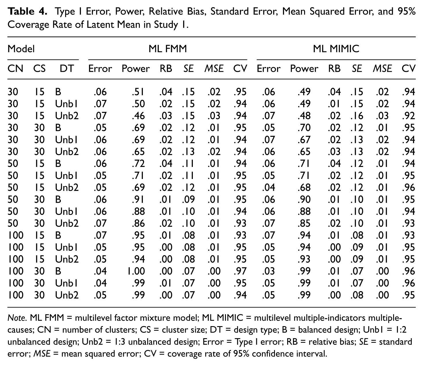
Table 4 summarizes Type I errors, power, relative bias, MSE, and 95% coverage of parameter estimation in Study 1. The performances of ML FMM and ML MIMIC were comparable in all evaluation criteria. Type I errors of ML FMM and MLMIMIC were properly controlled for regardless of small sample size and unbalanced design types. However, as expected, the power of both methods was very low for small sample size such as less than the combination of CN = 50 and CS = 15 (ranging from .51 to .72 for ML FMM and .48 to .71 for ML MIMIC), and it was increased to a reasonable level as the sample size increased. Also, the relative bias and 95% coverage rates of both methods were within the standard value of .1 and range of .91 to .97, respectively in all conditions. SE and MSE were not large in both methods and coverage rates of 95% CI for all conditions were within the appropriate range in both methods.
Type I Error, Power, Relative Bias, Standard Error, Mean Squared Error, and 95% Coverage Rate of Latent Mean in Study 1.
Note. ML FMM = multilevel factor mixture model; ML MIMIC = multilevel multiple-indicators multiple-causes; CN = number of clusters; CS = cluster size; DT = design type; B = balanced design; Unb1 = 1:2 unbalanced design; Unb2 = 1:3 unbalanced design; Error = Type I error; RB = relative bias; SE = standard error; MSE = mean squared error; CV = coverage rate of 95% confidence interval.
Results: Study 2
Convergence Rates
Similar patterns of convergence rates with Study 1 emerged. The convergence rates of two alternative ML FMM models were not different from each other and reached 1.0 or close to 1.0. ML MIMIC had a rather lower convergence rate (from 75.6% to 91.2%) than the ML FMM models. As with the results of Study 1, there were no significant differences across the factorial invariance testing models and simulation conditions. These results indicate that both methods can be easily applied in a modified form to complex models.
Power and Type I Errors of Factorial Invariance Testing Using Model Selection Criteria
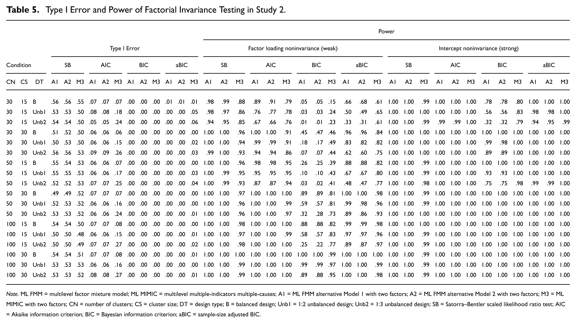
Table 5 presents the results of Type I errors and power of factorial invariance testing for ML FMM A1, ML FMM A2, and ML MIMIC with multilevel two-factor CFA model using model selection criteria (i.e., SB-LRT, AIC, BIC, and aBIC), respectively. The results of Study 2 were considerably similar to those of Study 1. The performances of ML FMM A1 and ML FMM A2 resulted in almost the same results, and the differences with ML MIMIC were negligible.
Type I Error and Power of Factorial Invariance Testing in Study 2.
Note. ML FMM = multilevel factor mixture model; ML MIMIC = multilevel multiple-indicators multiple-causes; A1 = ML FMM alternative Model 1 with two factors; A2 = ML FMM alternative Model 2 with two factors; M3 = ML MIMIC with two factors; CN = number of clusters; CS = cluster size; DT = design type; B = balanced design; Unb1 = 1:2 unbalanced design; Unb2 = 1:3 unbalanced design; SB = Satorra–Bentler scaled likelihood ratio test; AIC = Akaike information criterion; BIC = Bayesian information criterion; aBIC = sample-size adjusted BIC.
Generally, as in Study 1, the power of weak invariance model testing was poorer than that of the intercept invariance model testing. Alternative models of ML FMM tended to be more sensitive to uneven sample size conditions than ML MIMIC. In addition, Type I errors and power produced concordant results irrespective of sample size conditions.
Specifically, Type I errors of SB-LRT were unacceptably large regardless of the condition in all methods. Even though the power is excellent, it is not appropriate to consider the criteria for factor invariance testing. On the other hand, those of AIC, BIC, and aBIC were properly controlled for in all conditions at a nominal level except for AIC in the unbalanced condition in ML MIMIC. Accordingly, it can be considered a model selection criterion depending on sample size conditions in which power above a standard value is secured.
Except for a small sample size (CN = 30, CS = 15), the power of AIC was acceptable, whereas BIC and aBIC required a fairly large sample to have power above the standard of .8. BIC required a sample size of 1,500 (CN = 50, CS = 30) or higher for both methods, and 3,000 (CN = 100, CS = 30) if the sample size is unbalanced. aBIC was less demanding than BIC, and both methods required a sample size of 900 (CN = 30, CS = 30) or higher, and 1,500 (CN = 500, CS = 30) when the sample size between the comparison groups is unbalanced.
Power, Type I Errors, Bias, Mean Squared Error, and 95% Coverage of Latent Mean Difference Testing
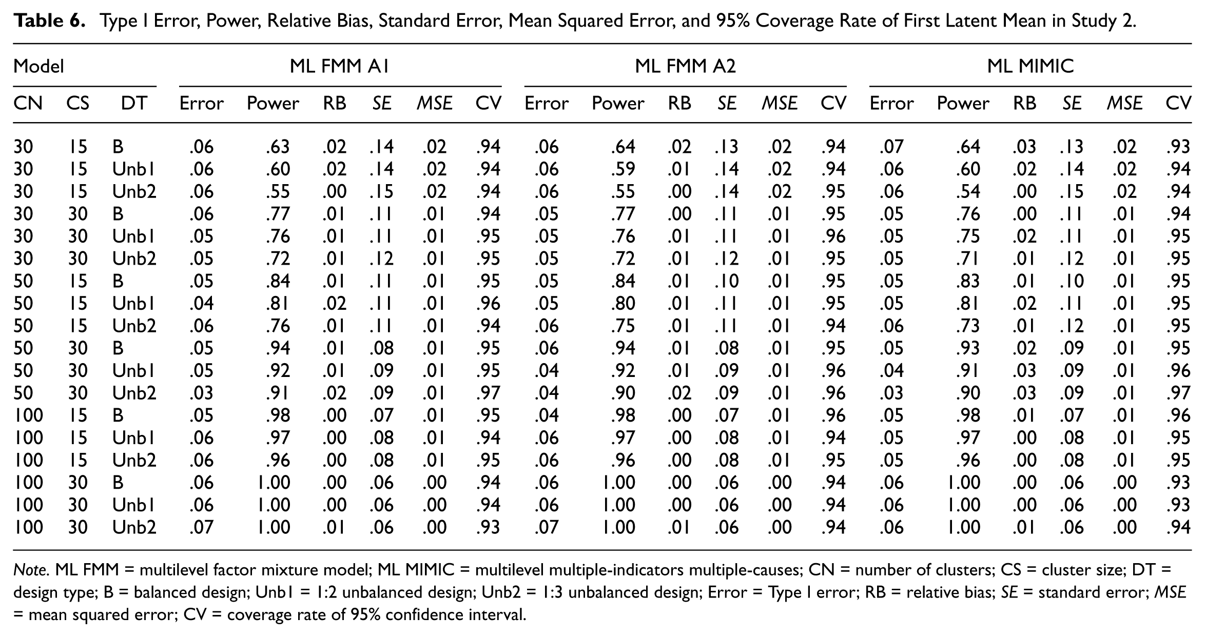
Table 6 summarizes Type I errors, power, relative bias, MSE, and 95% coverage of two latent mean parameter estimations. As in Study 1, the performance of two ML FMM alternative models and ML MIMIC in all evaluation criteria were comparable. Type I error rates were properly controlled and relative bias was below .05 in all conditions for both methods. Similar to Study 1, the power of both methods was low for a small sample size (i.e., less than CN = 50 and CS = 30), but as the sample size increased, the power also improved. But the only difference from Study 1 is that when the unbalanced degree of the sample size of the two comparison groups was not as large as 1:3, the condition of the combination of CN = 50 and CS = 15 also had a power of .8 or more.
Type I Error, Power, Relative Bias, Standard Error, Mean Squared Error, and 95% Coverage Rate of First Latent Mean in Study 2.
Note. ML FMM = multilevel factor mixture model; ML MIMIC = multilevel multiple-indicators multiple-causes; CN = number of clusters; CS = cluster size; DT = design type; B = balanced design; Unb1 = 1:2 unbalanced design; Unb2 = 1:3 unbalanced design; Error = Type I error; RB = relative bias; SE = standard error; MSE = mean squared error; CV = coverage rate of 95% confidence interval.
Discussion and Conclusion
Factorial invariance testing in multilevel data across within-level groups can be challenging due to the complexity of the model in relation to considering dependencies at the between level. This study addressed modeling and analysis issues in multilevel multiple group analysis when the grouping variable exists at the within level. Two methods have been considered to be suitable: ML FMM and ML MIMIC modeling. To investigate the performances of the proposed models regarding a set of factor invariance testing (i.e., weak and strong invariance testing) and subsequent latent group mean difference testing, two Monte Carlo studies were conducted. In Study 1, the performances of ML FMM and ML MIMIC were examined for multilevel one-factor CFA model. In Study 2, alternative models of ML FMM that are more restricted models (i.e., ML FMM A1 and A2) were suggested and their performance was compared with ML MIMIC for a multilevel two-factor CFA model. It is because when a research model is more complex (i.e., more than one factors or more than two groups), it is technically impossible to estimate all random group effects as in ML FMM.
The performance of the multiple group analysis on these methods was evaluated on two aspects. First, the performance of the factorial invariance testing was evaluated by setting noninvariance to either factor loadings or intercepts (i.e., weak and strong invariance model testing, respectively) for the two indicators. Second, to evaluate the performance of the latent group mean differences testing, a factorial invariance model in which there is a difference in the mean of the latent variable across within-level groups was simulated. In addition, factorial invariance model with a zero latent mean difference was also generated to assess the Type I error rates.
The major findings of the current study are summarized below to provide guidelines for applied researchers.
First, as expected based on previous studies, ML MIMIC had higher power than ML FMM for the small sample size condition. ML FMM needed more sample sizes than the ML MIMIC in order to obtain more than .8 power based on three ICs (i.e., AIC, BIC, and aBIC) in Study 1. Specifically, AIC using ML MIMIC had sufficient power regardless of the degree of unbalanced design under the small sample sizes condition of CN = 30 and CS = 15, whereas ML FMM’s power was secured only under balanced conditions. In BIC and aBIC, ML FMM required total sample sizes of 3,000 (CN = 100, CS = 30) and 1,500 (CN = 50, CS=30), respectively, whereas ML MIMIC was found to have power exceeding the standard value even under the relatively small sample size conditions of 1,500 (CN = 50, CS = 30) and 900 (CN = 30, CS = 30), respectively. These results are in line with previous studies (Kim & Cao, 2015; Woods, 2009) as the advantage of ML MIMIC for small sample sizes in multiple group analysis across within-level groups using multilevel data.
Second, as a result of examining the performance of SB-LRT, AIC, BIC, and aBIC as a criterion for detecting noninvariance, the performances of strong invariance testing were remarkably better than those of weak invariance testing across two studies. This result is not surprising in that the strong invariance testing is a more parsimonious model that constrains intercepts as well as factor loadings, implying that it is necessary to keep in mind that the conditions of weak invariance testing to reach the proper power in multiple group analysis are important. For both tests (i.e., weak and strong invariance testing), SB-LRT is not recommended due to unacceptably large Type I error rates. AIC showed the best performance among the three ICs criteria under small sample size condition. However, when the sample is an unbalanced type, AIC in the ML MIMIC results was found to be inappropriate for use as a model selection criterion due to unacceptably large Type I errors. BIC and aBIC generally functioned well under sufficiently large sample sizes conditions. To have adequate power in the multilevel one-factor model (Study 1), BIC required total sample of 3,000 (CN = 100, CS = 30) for ML FMM and 1,500 (CN = 50, CS = 30) for ML MIMIC. Also, aBIC required a smaller sample size than this, which was 1,500 (CN = 50, CS = 30) for ML FM and 900 (CN = 30, CS = 30) for ML MIMIC. Similar patterns were found in Study 2, and a proper power was reached even under smaller sample size conditions because of the more restrictive model than in Study 1. That is, when the comparison group size was balanced, in both methods, an appropriate power was reached when the total sample sizes were 1,500 (CN = 50, CS = 30) in BIC and 900 (CN = 30, CS = 30) in aBIC.
Third, to perform a series of factorial invariance testing and latent mean difference testing sequentially, the number of clusters is recommended to be at least 50 and ideally more than 100 in multilevel multiple group analysis across within-level groups. When the number of clusters is less than 50, the power of parameter estimation for the latent mean has not reached the standard value, and among the ICs used as a model selection criterion in factor invariance testing, only AIC can be used in a limited manner depending on the other conditions. This result was consistent with studies of sample sizes in MSEM (Hox et al., 2010; Hox & Maas, 2001; Maas & Hox, 2005). Besides the number of clusters, cluster size also contributes to increasing the total sample size, so it should be considered in the analysis, but it was confirmed that the number of clusters played a more important role in multilevel analysis. Comparing the two conditions of CN = 30, CS = 30 and CN = 50, CS = 15 in this study, the former condition is larger as the total sample sizes is 900 and 750, but the performance of the latter condition with a larger number of clusters was better across many conditions. In addition, in a comparison of the two conditions of CN = 50, CS = 30 and CN = 100, CS = 15 with the same total sample size, it was confirmed that the latter condition with a larger number of clusters has better performance than the former condition with a larger cluster size.
Fourth, as expected, if the sample size between groups is uneven, more samples should be obtained by considering the degree of unbalance. Under the minimum sample size conditions of CN = 30, CS = 15, the AIC of the two methods (i.e., ML FMM and ML MIMIC) secured power only in a balanced design but had low power under unbalanced conditions. However, if the sample sizes were large enough (CN = 100, CS = 30 in all three ICs), the uneven conditions were not an issue. It is not possible to conclude that the effects of the unbalanced design types are considerably critical given that the magnitude of the unbalanced set by the conditions in this study is not small at 2:1 and 3:1, but it is clear that researchers should consider it.
To sum up, there is a difference between the two methods in that ML MIMIC has the advantage of testing factorial invariance with small sample sizes. Whereas, the estimation is more difficult than ML FMM in that weak invariance testing takes longer to estimate by including interaction terms with latent variables, and in the case of multifactor models, it is necessary to test one by one for each factor. Nevertheless, the differences were not remarkable; therefore, both methods can be suitably used for multilevel multiple group analysis across within-level groups when researchers understand the performance patterns of the two methods and utilize the pros and cons.
Differentiation from previous studies and the implications of this study are as follows. First, this study compared two methods of ML FMM and ML MIMIC regarding sequential procedures (i.e., weak and strong invariance testing and latent means difference testing after holding for factorial invariance) in multiple group analysis and the performance in each procedure was evaluated integrally. Second, the current study confirmed by simulation that the design type in groups (i.e., balanced or unbalanced sample between the groups) is an important factor for the results of multiple group analysis. Third, given the fact that it was difficult to apply the standard analysis method (used in Study 1) to a complex model (e.g., multiple-factor or three or more groups comparison model), alternative models of ML FMM were presented and the performances were assessed. The major findings of Study 2 are expected to be generalizable to a more complex model. For example, ML FMM A1 or A2 can be applicable to a multilevel three-factor model or many groups analysis model.
The limitation of this study and future studies should be noted. First, in order to reflect the reality in the population model, heterogeneity (i.e., heterogeneous factor variance and residual variance) was assumed across within-level groups, and different factor loadings across within and between levels were set despite the cross-level factor loading constraint imposed on the analysis model. However, since they were not considered conditions (i.e., degree of heterogeneous variance and residual variance, degree of factor loading differences), overgeneralizations should be avoided. For example, when there are considerable differences in factor loading between levels, much deliberation is necessary for the application of these findings of the current study. Second, this study examined a model with an equal factor structure across levels (i.e., the same number of factors at both levels). When the model has unequal factor structures across levels, it is not possible to perform a factorial invariance testing in a multiple group approach that splits data by groups and imposes necessary constraints on each group. Not only is cross-level factor loading invariance required, but also intercept and latent group means are estimated at between level in multilevel multiple group analysis. In this case, a MIMIC approach that includes the group as a covariate can be more appropriate. In the MIMIC approach, all factorial invariance testing procedures are performed at the within level, in which the grouping variable exists, and latent group mean testing is also conducted at the corresponding level. Therefore, future studies will need to examine the performance of methods using ML MIMIC to models with unequal factor structures across levels.
Footnotes
Declaration of Conflicting Interests
The authors declared no potential conflicts of interest with respect to the research, authorship, and/or publication of this article.
Funding
The authors received no financial support for the research, authorship, and/or publication of this article.