
Abstract
This article studies the Type I error, false positive rates, and power of four versions of the Lagrange multiplier test to detect measurement noninvariance in item response theory (IRT) models for binary data under model misspecification. The tests considered are the Lagrange multiplier test computed with the Hessian and cross-product approach, the generalized Lagrange multiplier test and the generalized jackknife score test. The two model misspecifications are those of local dependence among items and nonnormal distribution of the latent variable. The power of the tests is computed in two ways, empirically through Monte Carlo simulation methods and asymptotically, using the asymptotic distribution of each test under the alternative hypothesis. The performance of these tests is evaluated by means of a simulation study. The results highlight that, under mild model misspecification, all tests have good performance while, under strong model misspecification, the tests performance deteriorates, especially for false positive rates under local dependence and power for small sample size under misspecification of the latent variable distribution. In general, the Lagrange multiplier test computed with the Hessian approach and the generalized Lagrange multiplier test have better performance in terms of false positive rates while the Lagrange multiplier test computed with the cross-product approach has the highest power for small sample sizes. The asymptotic power turns out to be a good alternative to the classic empirical power because it is less time consuming. The Lagrange tests studied here have been also applied to a real data set.
Introduction
Item response theory (IRT) models are used in psychological and educational research for measuring unobserved constructs, also known as factors or latent variables, from correlated observed variables/items. The main assumptions and features of an IRT model are (1) local independence among items conditional on the latent variable(s), (2) it is usually a parametric model for the probability of responding “correctly/positively” to an item given the latent variable(s) also known as response category probability and item characteristic curve (ICC), and (3) normal distribution for the latent variable(s) (Bartholomew et al., 2011). As with any statistical model, some of the above assumptions may be violated. The likelihood-ratio, the Wald, and the Lagrange multiplier or score (LM) test statistics (Cox and Hinkley, 1979) check model fit and they are asymptotically equivalent. Differently from the likelihood-ratio and the Wald test, the LM test only requires the computation of the restricted estimator (model under the null hypothesis). The LM test can be very convenient in IRT models, where multiple model violations (e.g., local dependence, nonnormality of latent distribution) can occur (Fox and Glas, 2005). The LM test does not need the estimation of an alternative model for each one of these violations. Moreover, there is model violation, such as differential item functioning (DIF), that requires testing items sequentially (Glas, 1998). The LM test does not require new parameter estimates for every tested item, making it computationally less intensive, especially in long tests. For these reasons, the LM test is used in IRT to detect DIF (Fox & Glas, 2005; Glas, 1998), local dependence (LD) (Fox and Glas, 2005; Glas, 1999; Glas & Falcón, 2003; Kim et al., 2011; Liu and Maydeu-Olivares, 2013; Liu & Thissen, 2012, 2014; Oberski et al., 2013; van der Linden & Glas, 2010) and deviation from the parametric model (i.e., ICC) (Glas, 1999; Glas & Falcón, 2003; Ranger & Kuhn, 2012).
The LM test depends on the Fisher information matrix. Different approximations of this matrix lead to different test performances. Accurate results for the LM test can be obtained by considering the expected Hessian and cross-product matrix, as shown in Liu and Maydeu-Olivares (2013), but they are unfeasible in long tests. For this reason, the observed versions of these matrices are preferred for the computation of the LM test. Some authors (Glas, 1998; Oberski et al., 2013) use the observed Hessian matrix, which we denote with LM(H), and others (Liu and Maydeu-Olivares, 2013; Liu & Thissen, 2012, 2014) the observed cross-product matrix, which we denote with LM(CP). Falk and Monroe (2018) compare both approaches. The LM(CP) test shows more inflated Type I error rates than the LM(H) test, especially with long tests and small sample size, but it is fast to compute (Falk & Monroe, 2018; Liu & Maydeu-Olivares, 2013; Liu & Thissen, 2012, 2014). In some works, the LM test statistic is applied in the case of model misspecification under the null and the alternative hypotheses, showing a good performance when the amount of model misspecification is overall small (Falk & Monroe, 2018; Glas & Falcón, 2003; Guastadisegni et al., in press). Different versions of the LM test are also derived under model misspecification (Boos, 1992; White, 1982). White (1982) proposes the generalized Lagrange multiplier (LM(S)) test, whose expression involves the sandwich variance and covariance matrix. Similarly Boos (1992) derives a generalized score (GS) test for least squares, robust M-estimation, and quasi-likelihood estimation methods that is equivalent to the LM(S) test when maximum likelihood (ML)-based methods are used. The generalized jackknife score (GS(J)) test is a version of the GS test, derived under model misspecification, where the covariance matrix of the score is computed using the jackknife estimates (J. Rao et al., 1998). The GS(J) test has not been studied in the IRT context. As far as we know, the LM(S) test is studied only by Falk and Monroe (2018) and Guastadisegni et al. (in press). Falk and Monroe (2018) compare the performance of the LM(S), LM(CP), and LM(H) tests for a single omitted cross-loading and Guastadisegni et al. (in press) compute the empirical and asymptotic power of the LM(S) and LM(H) tests to assess measurement invariance under misspecification of the latent variable distribution, without studying the Type I error/false positive rates of these two tests. Different from these works, we assess measurement invariance considering a more general framework, where the model misspecification is due to local dependence among items and different nonnormal latent variable distributions.
In the case of a one factor model, an item is measurement invariant if the conditional distribution of the item given the latent variable is independent of group membership identified by an external group variable (eg, sex, age, country) (Mellenbergh, 1982, 1983). An item is measurement noninvariant (also known as DIF), if it measures different abilities for different group memberships. In this case, the expected score of the item differs in the subgroups for the same level of the latent variable. Measurement invariance can be studied either in a multiple-group analysis setup (Jöreskog, 1971) or with the multiple indicator multiple causes (MIMIC) model (Jöreskog & Goldberger, 1975). The model allows direct and indirect effects of a binary group covariate on the probability of giving a “correct/positive” response to an item and on the latent variable respectively.
The contribution of this article is twofold. First, we assess item measurement invariance under model misspecification, using four versions of the LM test. The four versions differ in the form of the covariance matrix of the estimators. Mainly, the Hessian estimator (LM(H)), the cross-product estimator (LM(CP)), the sandwich estimator (LM(S)), and the jackknife estimator (GS(J)) are discussed and studied here. Second, we compute the power of the LM(H), LM(CP), and LM(S) tests in two ways, empirically through Monte Carlo simulation methods and asymptotically using the distribution of each test under the alternative hypothesis, which depends on a noncentrality parameter often difficult to compute (Gudicha et al., 2017). The noncentrality parameter is approximated using the procedure derived by Gudicha et al. (2017) for the Wald and likelihood-ratio tests and it is applied in Guastadisegni et al. (in press) to the LM(H) and LM(S) tests under misspecification of the latent variable distribution. We extend this method to the case of local dependence and to the LM(CP) test.
Through an extensive simulation study, we compare the performance of the different versions of the LM tests in terms of Type I error rate, false positive rate, and empirical and asymptotic power, varying the type and the misspecification level and considering single and multiple parameter hypotheses tests for measurement invariance. Moreover, we illustrate the use of these tests to a real data set.
The article is organized as follows. First, we present the MIMIC model with covariate effects. Second, we describe the four versions of the LM tests and the procedure to estimate the asymptotic power for the LM(H), LM(CP), and LM(S) tests. Next, we present a Monte Carlo simulation study and the results from the real data analysis. Finally, some concluding remarks are presented and discussed.
The MIMIC Model for Binary Data
Let us denote by
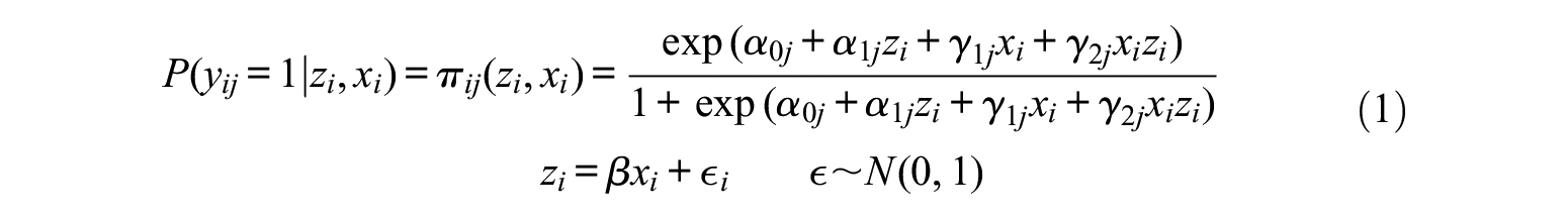
where
where
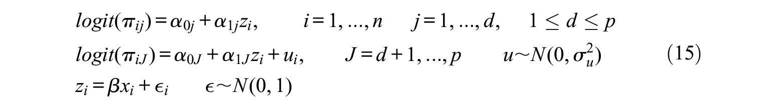
Uniform and nonuniform DIF for an item
Lagrange Multiplier Tests
The Classical Lagrange Multiplier Test
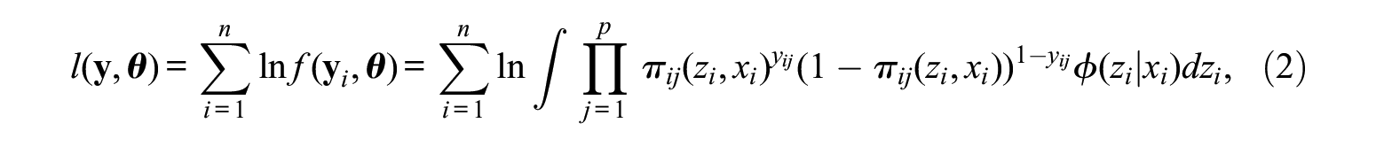
The LM test (C. R. Rao, 1948) evaluates the statistical significance of imposed restrictions on model parameters. We consider a sample

where
The LM statistic is (C. R. Rao, 1948):

where

where

and evaluated at
Two different versions of the LM test are studied here depending on which matrix is used for estimating

whereas the cross-product approach (LM(CP)), uses the observed cross-product matrix

Under correct model specification,
Under a correctly specified likelihood and under
To compute the local asymptotic power of the LM test, a standard approach is to consider a set of local alternatives close to the null value for large

The asymptotic power is computed as
Approximation Procedure for the Asymptotic Power
The asymptotic distribution of the LM test as a non-central chi-square with noncentrality parameter in equation (9) holds when the model defined under the set of local alternatives is true, that is, when the model under the null hypothesis is barely incorrect for large
From the model defined under the alternative hypothesis, create a large data set (e.g.,
Fit the model under
Take the value of the LM(H) or LM(CP) statistic as the estimate of the noncentrality parameter
Compute the noncentrality parameter for a sample of size 1 equal to
The noncentrality parameter for a sample of size
The asymptotic power of the LM(H) or LM(CP) test can be determined by comparing the
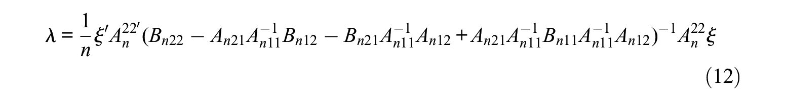
The Generalized Lagrange Multiplier Test
Consider a sample
Under model misspecification, the null and the alternative hypotheses are now specified in terms of

where
The Generalized Lagrange Multiplier test is defined as (Engle, 1984; White, 1982):

where
As before, the local asymptotic power of the LM(S) test is obtained by considering a set of local alternatives given by
where
The Jackknife Generalized Score Test
When ML-based methods are used, the LM(S) test derived by White (1982) is equivalent to the GS test derived by Boos (1992) under model misspecification and valid under different types of estimation methods, such as least squares, quasi-ML, and robust M-estimation. The Generalized Score test for the hypothesis testing given in (10) is

where
When likelihood-based methods are used,
J. Rao et al. (1998) proposed a version of the generalized score test in a general estimating equations framework (Godambe and Thompson, 1986) for a stratified multistage sampling design, based on a consistent jackknife estimator of

Simulation Study
We study the performance of the LM(H), LM(CP), LM(S), and GS(J) test statistics under no misspecification and misspecification either due to local dependence or in the latent variable distribution. Since the main focus of this work is the case of model misspecification, the results under correct model specification are reported in the Supplemental Material. Under a correct model specification, data are generated from the two-parameter logistic (2-PL) model (Birnbaum, 1968) with a linear structural model. When the model is correctly specified, we find results in line with the literature. In particular, the LM(CP) test shows inflated Type I error rates whereas the LM(H) and LM(S) tests have simulated Type I error rates quite close to the nominal level
In the Violation of Local Independence and the Misspecification of the Latent Variable Distribution sections, uniform and nonuniform DIF are studied in the simulation as well as single and multiple parameter hypotheses. The performance of the GS(J) test is evaluated in a separate simulation study in The study on the GS(J) Test section.
We consider the following simulation conditions: number of items
The optimization is conducted in R with the function “optim”, and numerical derivatives are obtained with the “NumDeriv” R package. In all the simulation scenarios,
Under model misspecification, in hypothesis testing we should account for the true data generating value
when
when
when
the case
To estimate the unknown parameters
Violation of Local Independence
Conditional dependence among certain items is introduced in the data generating model via a common individual specific random variables
Both for
To test for nonuniform DIF under model misspecification, we consider the following unconstrained model:

where items (
In our simulations, the model fitted to the data is given in (16) with parameters
This implies that one item is tested for uniform DIF.
where
One item is tested for nonuniform DIF.
One item is tested for uniform DIF.
Five items are tested for uniform DIF.
One item is tested for nonuniform DIF.
Table 1 presents the false positive rates for the LM(H), LM(CP), and LM(S) tests under local dependence for Scenarios A, B, and C.
False Positive Rates of The LM(H), LM(CP), and LM(S) Tests Under Scenarios A, B, and C,
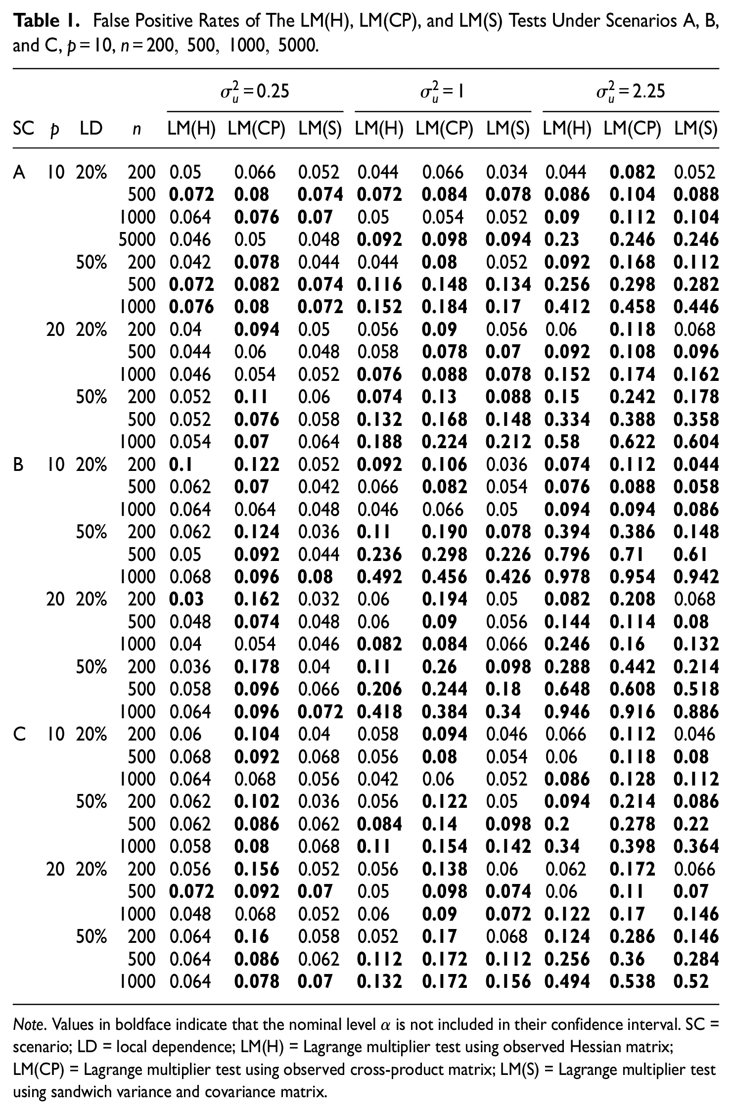
Note. Values in boldface indicate that the nominal level
In the majority of cases, we can see that when the variance of the random effect is low (
Table 2 presents the empirical and asymptotic power for the LM(H), LM(CP), and LM(S) tests under local dependence for Scenario D.
Empirical Power (EP) and Asymptotic Power (AP) of the LM(H), LM(CP), and LM(S) Tests Under Scenario D,
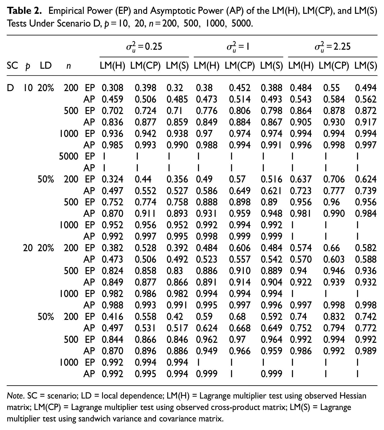
Note. SC = scenario; LD = local dependence; LM(H) = Lagrange multiplier test using observed Hessian matrix; LM(CP) = Lagrange multiplier test using observed cross-product matrix; LM(S) = Lagrange multiplier test using sandwich variance and covariance matrix.
Overall, there are some numerical differences between the asymptotic and empirical power that decrease with the increase in the number of items and the sample size. It is worth noting that the behaviour of the empirical and asymptotic power is the same. Indeed, according to both methods, LM(CP) has the highest power and LM(H) and LM(S) have a very similar power under all conditions. The empirical and asymptotic power increases with both the sample size and the number of items. Since there are no substantial differences between the two procedures, only the empirical power is computed for Scenarios E and F. Table 3 presents the empirical power for the LM(H), LM(CP), and LM(S) tests under local dependence for Scenarios E and F.
Empirical Power of the LM(H), LM(CP), and LM(S) Tests Under Scenarios E and F,
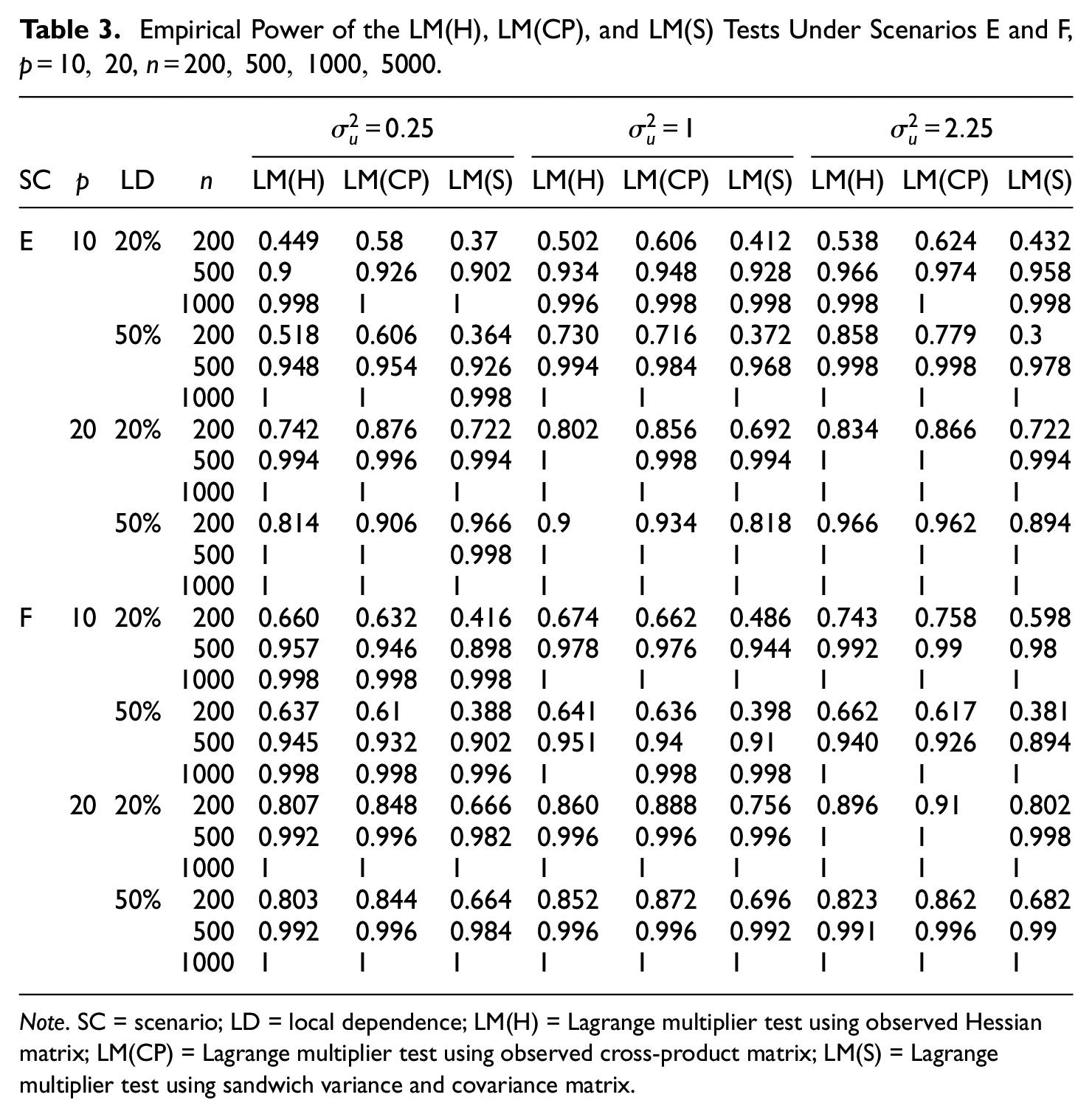
Note. SC = scenario; LD = local dependence; LM(H) = Lagrange multiplier test using observed Hessian matrix; LM(CP) = Lagrange multiplier test using observed cross-product matrix; LM(S) = Lagrange multiplier test using sandwich variance and covariance matrix.
Under the multiple parameters scenarios (E and F) and small sample sizes (
Misspecification of the Latent Variable Distribution
The data are generated from the following model:

Three different distributions are assumed for the latent variable. Namely, the error term is generated from a mixture of normals as

where
Intercepts (
Table 4 reports the false positive rates for the LM(H), LM(CP), and LM(S) tests under misspecification of the latent variable distribution for Scenarios A, B, and C.
False Positive Rates of the LM(H), LM(CP), and LM(S) Tests Under Scenarios A, B, and C,

Note. Values in boldface indicate that the nominal level
The misspecification of the latent variable distribution in the case of a mixture of normals does not affect the false positive rates of the LM(H) and LM(S) tests, whereas the LM(CP) test has inflated false positive rates, especially under Scenarios B and C. When
Table 5 presents the empirical and asymptotic power for LM(H), LM(CP), and LM(S) tests under misspecification of the latent variable distribution for Scenario D.
Empirical Power (EP) and Asymptotic Power (AP) of the LM(H), LM(CP), and LM(S) Tests Under Scenario D,
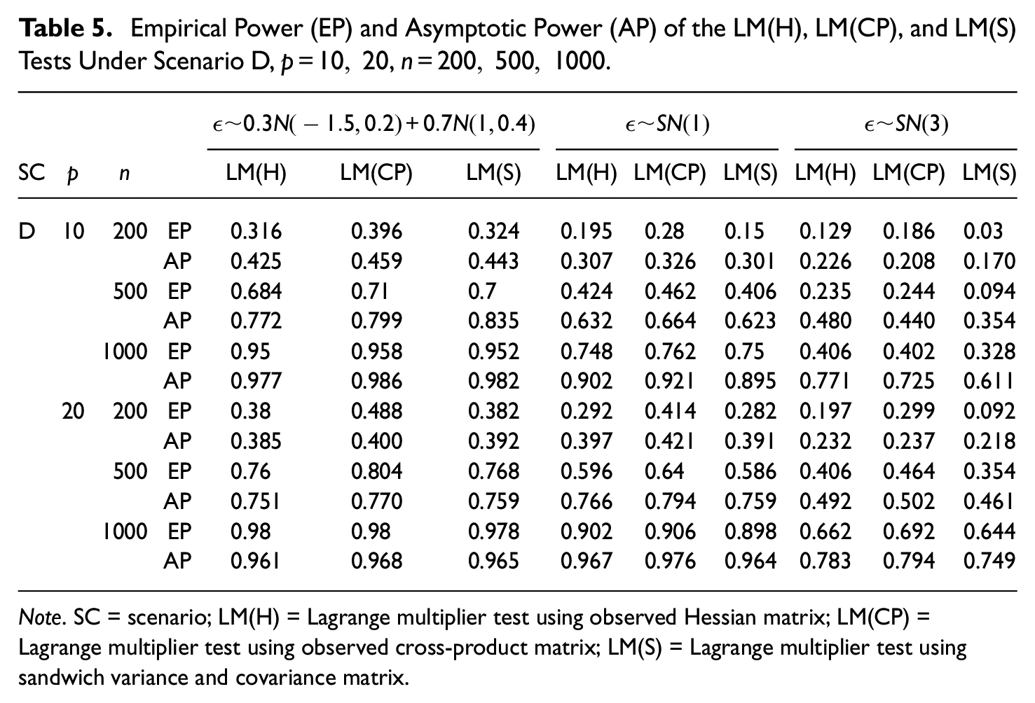
Note. SC = scenario; LM(H) = Lagrange multiplier test using observed Hessian matrix; LM(CP) = Lagrange multiplier test using observed cross-product matrix; LM(S) = Lagrange multiplier test using sandwich variance and covariance matrix.
Overall, the numerical differences between the asymptotic and empirical power are small. As in the case of local dependence, the empirical and asymptotic power give the same information. For Scenario D and large sample sizes, the power of all tests is not affected by the latent variable having a mixture of normal distributions. When
Table 6 presents the power for LM(H), LM(CP), and LM(S) tests under misspecification of the latent variable distribution for Scenarios E and F.
Empirical Power of the LM(H), LM(CP), and LM(S) Tests Under Scenarios E and F,
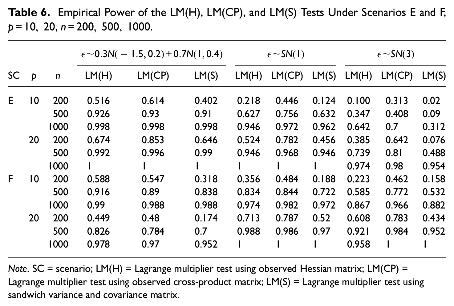
Note. SC = scenario; LM(H) = Lagrange multiplier test using observed Hessian matrix; LM(CP) = Lagrange multiplier test using observed cross-product matrix; LM(S) = Lagrange multiplier test using sandwich variance and covariance matrix.
Similarly to the false positive rates study, the power of all tests studied here is not affected by the latent variable having a mixture of normal distributions and it is lower for small sample sizes. Interestingly, when
The Study on the GS(J) Test
The GS(J) test is computationally expensive compared with the other tests. Indeed, in each replication of a sample of size
Type I Error/False Positive racte of the GS(J), LM(H), LM(CP), and LM(S) Tests Under Scenario A,

Note. Values in boldface indicate that the nominal level
The GS(J) test and the LM(S) test perform similarly under all conditions. In general, all tests have good performance and only the LM(CP) test shows inflated false positive rates under some conditions.
Table 8 presents the empirical power for the GS(J), LM(H), LM(CP), and LM(S) tests under correct model specification, local dependence, and incorrect distribution of the latent variable, for Scenario A.
Empirical Power of the GS(J), LM(H), LM(CP), and LM(S) Tests Under Scenario A,
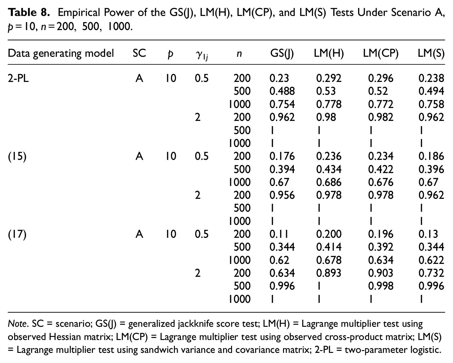
Note. SC = scenario; GS(J) = generalized jackknife score test; LM(H) = Lagrange multiplier test using observed Hessian matrix; LM(CP) = Lagrange multiplier test using observed cross-product matrix; LM(S) = Lagrange multiplier test using sandwich variance and covariance matrix; 2-PL = two-parameter logistic.
Under all conditions for small sample size, the power of the GS(J) test is always equal to or lower than the one of the LM(S) test. When the sample size increases, the two tests reach the same power. Similarly to the Type I error/false positive rate study, the performance of the GS(J) test is never superior to that of the other tests. For this reason, and for its high computational cost, we do not use the GS(J) test in the real data analysis.
An Application to a Real Data Set
In this section, we assess measurement invariance under model misspecification through the LM(H), LM(CP), and LM(S) tests on a real data set, taken from Miller et al. (1984). We select the same sample of observations and items analyzed by Duncan (1979). In 1953, in the Detroit Area, the following questions regarding sex role expectations were asked to a sample of 257 women: Here are some things that might be done by a boy or a girl. As I read each of these to you, I would like you to tell me if it should be done as a regular task by a boy, by a girl, or by both: (1) Shoveling walks, (2) Washing the car, (3) Dusting furniture, (4) Making beds.
Responses of “boy” to Items 1 and 2 and “girl” to Items 3 and 4 are coded as “0” and refer to traditional answers. Responses of “both” for all items are coded as “1” and refer to “egalitarian” answers. For the same sample of women, in addition to the four binary items, we consider a group variable, that we call “Work,” taken from the original data set (Miller et al., 1984). The following question was asked to the sample of mothers “What is your occupation? What kind of business is that in?” The possible responses were the following: “Professional, technical, and kindred workers”, “Managers, officials and proprietors, except farm”, “Clerical and kindred workers”, “Sales workers”, “Operatives and kindred workers”, “Private household workers, service workers”, “Laborers, except farm and mine”, and “Not in labor force”. We group these responses into two classes:
Class coded as “0”, which includes only answers “Not in labor force”. This class includes the group of nonworking women (
Class coded as “1”, which includes all the other responses. This class includes the group of working women (
The percentages of “egalitarian” answers among the group of nonworking women are 31%, 31%, 29% and 42% to Items 1 to 4, respectively. The percentages of “egalitarian” answers among the group of working women are 43%, 29%, 50% and 55% to Items 1 to 4, respectively. Women in the working group give more “egalitarian” answers than women in the nonworking group, especially to Items 3 and 4. The data set is analyzed by Mavridis and Moustaki (2009) and Irincheeva (2011). They show that the classical unidimensional IRT model with the latent variable distributed as a standard normal has a poor fit on this data set. Irincheeva (2011) estimates a semi-nonparametric (SNP) unidimensional IRT model to the data, that allows for more flexibility in the shape of the latent variable distribution, and gives a better fit of the proposed model to the data compared with the classic unidimensional IRT model. Moreover, the results found by Irincheeva (2011) suggest that the shape of the true latent variable is right skewed or even more complex.
Starting from these results, in this study we consider a unidimensional IRT model for binary data based on the assumption of standard normal latent variable distribution under the null hypothesis, that we know to be misspecified. Measurement invariance on the intercept of each item is tested through
The first step of the bootstrap hypothesis testing procedure is to generate
Calculate the statistic
Calculate the statistic
Compute the bootstrap p value as
Reject the null hypothesis if
When
Table 9 presents the p values for the LM(H), LM(CP), and LM(S) tests based on their theoretical distributions (TD) under the null hypothesis and on bootstrap hypothesis testing (BH) for measurement invariance on the item intercept and slope.
Theoretical Distributions (TD) and Bootstrap Hypothesis Testing (BH) p Values of the LM(H), LM(CP), and LM(S) Tests for Measurement Invariance on the Item Intercept and Slope.
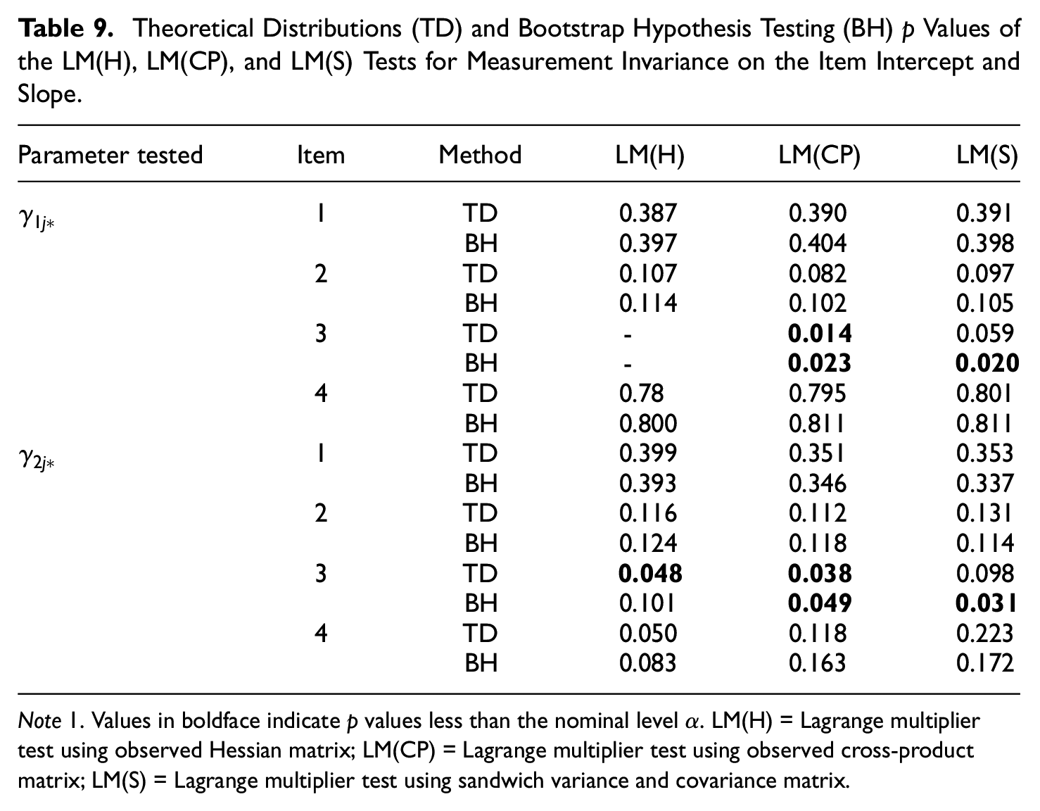
Note 1. Values in boldface indicate p values less than the nominal level
For all tests, TD and BH do not reject the null hypothesis of intercept and slope invariance for Items 1, 2, and 4. This is consistent with the simulation results, in which the false positive rates are less affected than the power of the tests by the misspecification of the latent variable distribution. However, BH and TD disagree for Item 3. Interestingly, only the LM(CP) test produces similar results to the BH p values of the LM(S) test, rejecting the null hypothesis of measurement invariance on the intercept and slope. This is consistent with the simulation results, where the LM(CP) test has the highest power for small sample sizes under misspecification of the latent variable distribution. The bootstrap hypothesis testing procedure for the LM(S) and LM(CP) tests turns out to be a good instrument to make a clearer decision on the acceptance or rejection of the null hypothesis, especially when these tests show contradictory results. By contrast, the LM(H) test gives negative statistics in the real data set and in a large number of bootstrap replications, as in some simulation scenarios under high misspecification of the latent variable distribution and small sample size. This makes it difficult to interpret results and worsens the performance of the bootstrap hypothesis testing procedure. Indeed, for measurement invariance on the intercept of Item 3, the TD and BH p values of the LM(H) test cannot be computed because the statistic calculated in the real data set is negative. Moreover, in the measurement invariance testing of the slope of Item 3, the result of the BH p value of LM(H) test is not stable because in 11.5% of the bootstrap replications we obtain nonvalid statistics that have been excluded from the BH p value computation.
Discussion
In this work, we evaluated the performance of the LM(H), LM(CP), LM(S), and GS(J) tests to assess measurement invariance under both correct model specification and different types of model misspecification by means of a wide simulation study and in a real data analysis. Moreover, we computed the empirical and asymptotic power of the LM(H), LM(CP), and LM(S) tests, using for the latter the asymptotic distributions of the statistics under the alternative hypothesis.
Under model misspecification, there are some differences between the three tests due to the type and the strength of the model misspecification. Under low local dependence, and when the latent variable is generated from a mixture of normals or from a moderate skew-normal, all tests have good performance in terms of false positive rates and power for large sample sizes. Only the LM(CP) test shows inflated false positive rates in some cases. For this reason, under mild model misspecification, we discourage the use of the LM(CP) test due to its inflated false positive rates. When the misspecification is high, the tests performance deteriorates. Indeed under high local dependence the false positive rates for all tests are seriously inflated while, when the latent variable is highly skewed, with 10 items and for small sample sizes, the LM(H) and LM(S) tests have very low power. Under high model misspecification, the LM(CP) test has the highest power for small sample sizes. It is worth noting that the LM(S) test, although derived under model misspecification, does not have better performance than the LM(H) test, particularly in terms of power but it always produces valid statistics. Under all types of misspecification considered, we do not find significant differences in the tests’ behavior between the case of measurement invariance on the intercept and that on the intercept and slope, both in single and multiple parameter hypothesis testing.
The simulation study highlights that there are small numerical differences between the asymptotic power, computed through the approximation method for the noncentrality parameter, and the empirical power. However, the results given by the two procedures are coherent and the asymptotic power can be a valid alternative to obtain the power of a test, since it allows us to reduced the time complexity compared with the empirical power.
Concerning the GS(J) test, it is never superior to the other tests and, due to its high computational cost, we do not recommend the use of this test to assess measurement invariance under model misspecification.
Consistently with the simulation results, in the real data analysis the LM(CP) test has the highest power to detect item measurement noninvariance under high misspecification of the latent variable distribution. The bootstrap hypothesis testing procedure turns out to be a good instrument under model misspecification. Indeed, it helps to make a clearer decision on the acceptance or rejection of the null hypothesis when the asymptotic tests provide contradictory results.
For further studies on the performance of the LM tests under model misspecification, different types of estimation methods could be considered. Moreover, we found that when data are generated assuming a skew-normal distribution for the latent variable, parameter estimates are seriously biased with respect to the true parameters’ values. Further research should be devoted to exploring misspecified models where the parameter estimates are consistent with regard to the true parameter values. In these cases, the LM tests should have a better performance.
Footnotes
Declaration of Conflicting Interests
The authors declared no potential conflicts of interest with respect to the research, authorship, and/or publication of this article.
Funding
The authors received no financial support for the research, authorship, and/or publication of this article.
Supplemental Material
Supplemental material for this article is available online.
References
Supplementary Material
Please find the following supplemental material available below.
For Open Access articles published under a Creative Commons License, all supplemental material carries the same license as the article it is associated with.
For non-Open Access articles published, all supplemental material carries a non-exclusive license, and permission requests for re-use of supplemental material or any part of supplemental material shall be sent directly to the copyright owner as specified in the copyright notice associated with the article.