On Effect Size Measures for Nested Measurement Models

Abstract

A class of effect size indices are discussed that evaluate the degree to which two nested confirmatory factor analysis models differ from each other in terms of fit to a set of observed variables. These descriptive effect measures can be used to quantify the impact of parameter restrictions imposed in an initially considered model and are free from an explicit relationship to sample size. The described indices represent the extent to which respective linear combinations of the proportions of explained variance in the manifest variables are changed as a result of introducing the constraints. The indices reflect corresponding aspects of the impact of the restrictions and are independent of their statistical significance or lack thereof. The discussed effect size measures are readily point and interval estimated, using popular software, and their application is illustrated with numerical examples.

Keywords

confidence interval confirmatory factor analysis effect size nested model parameter restriction proportion explained variance

Since its introduction about a half century ago, confirmatory factor analysis (CFA) has rapidly grown in popularity across the educational, behavioral, social, marketing, organizational, and biomedical sciences (e.g., Jöreskog, 1967). A key feature of this modeling approach is that it permits accounting for measurement error in studied construct indicators, is useful for developing complex measurement models for underlying latent dimensions of interest, and helps to examine theories about substantively important concepts and their interrelationships (e.g., Bollen, 1989). In addition, a particular strength of CFA is the opportunity it offers to scholars concerned with evaluating theoretical propositions reflected in corresponding parametric constraints (e.g., Millsap, 2012).

Model parameter restrictions are frequently utilized in applications of CFA in educational and behavioral research. For example, the equality of factor loadings pertaining to two or more indicators of an examined latent construct will often be of theoretical and empirical concern. This is because their identity represents the hypothesis of true score-equivalence (tau-equivalence) that is oftentimes of particular interest to examine as it can reflect, for instance, a characteristic feature of the popular Rasch model or a setting where the widely used coefficient alpha equals scale reliability at the population level (e.g., McDonald, 1999; Raykov & DiStefano, 2021). In addition, the test of tau-equivalence in a congeneric model (Jöreskog, 1971) permits scientists to select more parsimonious measurement models for studied latent variables, which may be involved in more general structural equation or latent variable models employed subsequently (e.g., Raykov & Marcoulides, 2006). Similarly, multiple population studies including one or more unobserved dimensions will be considerably facilitated, and their validity enhanced, if the loading and intercept group equality restrictions are plausible in relevant multigroup factor analysis models (e.g., Mulaik, 2009). The reason is that these restrictions represent what may be considered a necessary condition for measuring the same latent constructs in the examined populations (cf., Raykov et al., 2013). Testing these and other types of parametric constraints can therefore constitute an integral part of the process of the CFA-based study of important measurement-related research questions for behavioral and social scientists.

A consequential limitation of CFA and structural equation modeling applications more generally, however, is that, with increasing sample size, the pertinent restriction tests tend to be associated with significant results that may be spurious (cf. Schmidt, 1996). Consistent with other statistical hypothesis testing situations, when sufficiently large samples are available, a parametric constraint that is violated to a substantively trivial extent in a population under investigation will tend to be associated with a significant test finding (e.g., Casella & Berger, 2002). Such a result typically lacks subject matter meaning, is difficult if at all possible to interpret in content-domain terms, and may well be substantively uninformative for the researcher conducting the test within conventional CFA applications. For example, under normality, the popular likelihood ratio test (LRT; for example, Agresti, 2002) can be spuriously associated with a significant result in a large sample (see, for example, illustration section). At the same time, however, this finding may be reflecting mostly, if not exclusively, the sample size effect that is entangled with a potentially trivial and empirically meaningless violation(s) of the examined parameter restriction. Empirical settings where these circumstances may become relevant are increasingly more frequently encountered in contemporary educational and behavioral research. This marked trend is in particular due to the growing interest and popularity of complex design, nationally representative, and large-scale studies (e.g., Heeringa et al., 2017). All of them are usually based on samples with sizes well into the thousands from populations of research interest. For this reason, it is particularly important to be in a position to properly deal with the potential of spurious findings when examining various parametric constraints in these and other studies involving large samples. Therefore, alternative quantification of the effect of restrictions introduced in initially considered CFA models is desirable to evaluate corresponding subject-domain hypotheses in substantively meaningful terms. Such quantification can be offered by suitably developed effect size measures (cf. Grissom & Kim, 2012) that focus on the practical importance-related interpretability of the consequences of imposing the parameter restraints that produce two or more nested models under consideration.

To respond to this need, the following discussion is concerned with a class of effect size (ES) measures that index the respective degree to which two nested CFA models differ from each other in terms of their fit to a given set of analyzed observed variables, such as latent factor or studied construct indicators. The indices reflect the effects of parametric restrictions implemented in originally considered models and are each developed, so as to be free from an explicit relationship to sample size. They accomplish this aim by representing the extent to which suitable functions of the proportions explained variance for the manifest variables are changed as a consequence of imposing the constraint in question. Based on this feature, the described ES indices (a) inform the researcher about the substantive importance of the restriction under consideration, (b) are not impacted by statistical significance or lack thereof of the constraint, and (c) are directly extended and applicable with more general structural equation and latent variable models. These ES measures are readily point and interval estimated using popular latent variable modeling software and their application in CFA studies is illustrated with a pair of numerical examples.

Background, Notation, and Assumptions

In the remainder of this article, we assume that a set of p (approximately) continuous observed variables are given, which will be denoted X₁, X₂, . . ., X_p (p>2; compare Raykov & Calvocoressi, 2021). These variables may be some or all components of a psychometric scale or test under consideration, or alternatively part of or an entire inventory, composite, questionnaire, survey, test-battery, or self-report. We posit that their number is fixed, that is, X₁, X₂, . . ., X_p are given beforehand and are the only manifest variables of concern rather than sampled from a larger pool or universe of components/items that one wishes to make inferences to. In addition, X₁, X₂, . . ., X_p are presumed to have been administered to a sample from a studied population of units of analysis (e.g., students, subjects, persons, patients, employees, or respondents) that is not characterized by clustering effects or substantial unobserved heterogeneity (e.g., Raykov et al., 2016). Furthermore, we stipulate that the common factor model is valid for them (e.g., Mulaik, 2009), that is,

\underline{X} = \underline{μ} + Λ \underline{η} + \underline{δ}

(1)

holds, where X is the p× 1 vector of these measures and µ is the p× 1 vector of their means (with underlining used to denote vector; cf. Jöreskog & Sörbom, 1996). In Equation 1, Λ = [λ_ij] is the p×m factor loading matrix with entries λ_ij where m is an a priori known or given integer number (1≤m < p– 1), which matrix may, but need not, include cross-loadings (i = 1, . . ., p, j = 1, . . ., m). Moreover, η is the m× 1 vector of common factors there, denoted η₁, . . ., η_m, which are assumed with mean 0 and unit variance as well as possessing an unconstrained positive definite m×m covariance matrix Φ = [φ_uv] (u, v = 1, . . ., m). In addition, δ represents the p× 1 vector of unique factors (residual or error terms) that are assumed uncorrelated with the m factors and themselves associated with a positive definite covariance matrix Ψ = [ψ_gh] (g, h = 1, . . ., p). In multigroup studies, a direct extension of the model is defined in Equation 1 and this discussion is to be considered (e.g., Bollen, 1989), with the developments in the following sections being directly applicable then. Finally, all CFA models used or referred to in the rest of this article are testable with respect to their fit to analyzed data sets, and are assumed to be identified (if needed, by additional parameter restrictions that themselves are not of concern or dealt with in the sequel) as well as associated with admissible solutions once fitted to data.

ES Measures of Parameter Constraint Impact in Nested Models

In the described CFA setting, consider two nested CFA models that will be denoted M1 and M2. (The remaining discussion is directly extended to the case of more than two nested models, which is thus not explicitly pursued in what follows.) Assume that M2 is nested in M1, that is, M2 is obtained from M1 by imposing a constraint in M1 involving at least one (and usually two or more) of its parameters. The constraint may but need not be representable as a linear restriction, and may involve any (integer) number of parameters in M1. For example, as in the following illustration section, a constraint of interest may be stating the equality of q factor loadings in M1, which yields M2 (q>1). Similarly, in a two-group setting, a restriction of concern may be that of cross-group identity in some or all factor loadings involved in Model 1 (formally, in its two-group extension then), as, for instance, in measurement invariance studies (e.g., Millsap, 2012).

As indicated earlier, when tested, the parameter constraint that produces M2 as nested in M1 may turn out to be spuriously significant, that is, associated with a significant statistical hypothesis testing result, whereas the restriction violation has no meaningful substantive interpretation or practical importance. In particular, with a (sufficiently) large sample, a restriction that is trivially violated in a studied population may entail a significant finding mostly, if not exclusively, because of the size of the sample (e.g., Schmidt, 1996). More concretely, a constraint that for all empirical purposes may be treatable as satisfied in the population, while not being completely correct (unbeknownst to the researcher), may turn out to be significant, purely due to a large enough sample size (examples are provided in the illustration section.) In those cases, the scholar needs to be in a position to assess the effect of the parameter restriction when introduced in M1, rather than rely on the statistical testing procedure and possibly incorrectly infer from its spurious result that the examined constraint is not valid or plausible at large. That is, it is necessary to use then a substantively meaningful index of the consequences of imposing the constraint in Model M1, which quantity should not be affected by a potentially misleading significance result pertaining to that restriction.

A class of ES measures accomplishing this goal can be obtained by focusing on the popular proportion explained variance index. Accordingly, as one such measure, a researcher may consider the index ε₁ defined as follows:

ε_{1} = {R^{2}}_{a 1} - {R^{2}}_{a 2},

(2)

where

{R^{2}}_{a 1} = ({R^{2}}_{11} + {R^{2}}_{21} + \dots + {R^{2}}_{p 1}) / p

(3)

is the average R-squared index for the p observed variables X₁ through X_p in Model M1, while

{R^{2}}_{a 2} = ({R^{2}}_{12} + {R^{2}}_{22} + \dots + {R^{2}}_{p 2}) / p

(4)

is their average R-squared index in Model M2 (cf. Raykov & Calvocoressi, 2021). In Equations 3 and 4, each of the respective R-squared indices in their right-hand sides is the familiar and widely used proportion of variance in the respective response variable, which is explained by one or more independent variables that the former is related to in a model under consideration, and is readily provided by popular software when that model is fitted to data (e.g., Muthén & Muthén, 2021). For example, in a single-factor model, this R-squared index is defined as R² = λ²/(λ²+θ) for any construct indicator (when assuming unit latent variance, as in this article), where λ is its loading on the factor and θ is the associated unique variance (residual variance). In a model with two or more factors, this R-squared index is formally defined in the same way with respect to the pertinent factor in case of no cross-loadings, or its numerator and denominator are extended by the squared additional cross-loadings and twice all pertinent pairwise loading products with the factor correlations (cf. Raykov & Marcoulides, 2016).

The ES index ε₁ assigns the same weight of 1/p to all manifest variable R-squared indices. A natural extension of ε₁ is the weighted index ε₂ that is defined as follows:

ε_{2} = w_{1} {R^{2}}_{11} + w_{2} {R^{2}}_{21} + \dots + w_{p} {R^{2}}_{1} - (w_{1} {R^{2}}_{12} + w_{2} {R^{2}}_{22} + \dots + w_{p} {R^{2}}_{p 1}),

(5)

where the weights w₁ through w_p are prespecified nonnegative constants summing to 1, that is, with the property that w₁+. . .+w_p = 1. These weights can be suitably chosen, for instance, based on substantive and/or other relevant considerations (see below).

As a generalization of the quantity in Equation 5, a closely related ES index may use different sets of weights for Model M1 relative to the weights for Model M2, while within model these weights sum up to 1 as aforementioned:

ε_{3} = w_{11} {R^{2}}_{11} + w_{21} {R^{2}}_{21} + \dots + {w_{p}}_{1} {R^{2}}_{1} - (w_{12} {R^{2}}_{12} + w_{22} {R^{2}}_{22} + \dots + {w_{p}}_{2} {R^{2}}_{p 1}),

(6)

with w₁₁+ . . . +w_p₁ = w₁₂+ . . . +w_p₂ = 1 holding. One possible choice to consider along these lines is of the weights in Equation 6 being the corresponding ratios of the individual R-squared indices, per model, to the overall sum of R-squared across all observed variables in it, that is, as

w_{jg} = {R^{2}}_{jg} / ({R^{2}}_{1 g} + {R^{2}}_{2 g} + \dots + {R^{2}}_{pg}),

(7)

where j = 1, . . ., p is the observed variable subindex; while g = 1, 2 is the model subindex. (We note in passing that the sum of the weights [7] across all observed variables in a given model is 1; for examples, see illustration section.)

As additional informative options, any ES index from the aforementioned three, ε₁ through ε₃, may only involve manifest variables that are “affected” by a parameter constraint of interest. More specifically, if one were to be concerned with evaluating the impact of introducing the restriction of equality on say only q factor loadings, rather than on all p loadings in a CFA model, with q < p (for instance, in a model without cross loadings, and similarly in more general models; q≥ 1), then in the right-hand sides of the aforementioned defining equations for each of the indices ε₁ through ε₃ one may involve only the R-squared of the observed variables pertaining to these loadings, that is, the loadings of the “affected variables.”¹ For example, assuming without loss of generality that these q loadings are associated with the first q observed variables, X₁ through X_q, in a single-factor model, then the resulting version ε_1,q of the first described ES measure say, ε₁, is defined as

ε_{1, q} = ({R^{2}}_{11} + {R^{2}}_{21} + \dots + {R^{2}}_{q 1}) / q - ({R^{2}}_{12} + {R^{2}}_{22} + \dots + {R^{2}}_{q 2}) / q,

(8)

and similarly for the other two ES indices, ε₂ and ε₃. Equation 8, similar to the respective versions of ε₂ and ε₃ as well as those previously discussed, defines ES indices obviously also for the cases when the constraint of concern includes error variances in addition to, or instead of factor loadings (see Note 1).² A special case of the preceding developments that can also, or instead of the aforementioned indices, be of interest in an empirical study is obtained when all weights but one, say the jth, are selected as 0 (1 ≤j≤p; note that w_j = 1 in that case). Then Equation 8 yields the change in the respective individual measure R-squared as a result of introducing a respective parametric restriction (cf. Raykov & Zajacova, 2012).

Based on their formal definition in Equations 2 through 8, and earlier discussion, we note that none of the described ES measures depends on the statistical significance or lack thereof for the underlying parameter constraint. The reason is that these measures are by construction functions of R-squared indices that as proportions from observed sample variance are descriptive quantities and hence unaffected by statistical inferences and their results. Therefore (so long as the weights are chosen as prefixed constants as aforementioned), these R-squared values are independent of statistical significance results, and thus none of these ES measures is impacted by such results. We also mention that, while the context in which these measures are proposed here is that of nested measurement models, that is, a CFA setting, the same definitional equations can be applied in any structural equation model, resulting as a special case of the general LISREL model (e.g., Jöreskog & Sörbom, 1996), with at least one observed dependent variable. This is because the definition of the ES measures does not use (explicitly) information about the actual model being considered, and hence their formal definition is valid for any such LISREL model. Similarly, none of the aforementioned ES measures depends explicitly on sample size due to the fact that no R-squared index involved in them does by its definition.³

Unless a researcher has strong substantive or other reasons to prefer one or more of the ES measures defined in Equations 2 through 8, which reasons are deferred to the experts in the subject domain of application, the described ES indices are, in general, best treated as providing complementary information with respect to the impact of nesting parameter restrictions in CFA models. Their utilization in an empirical study may also involve a judicious choice among them, if beneficial, by the educational or behavioral scientist, possibly based on substantive expert considerations that could be idiosyncratic to the study.

The discussion up to this point has evolved exclusively at the population level. In empirical research, sample point and interval estimation of the described ES measures is readily accomplished, using the popular software Mplus (Muthén & Muthén, 2021) and Stata (Stata Base Reference Manual, 2019; see illustration section and Appendices A through D). This software application includes, in particular, the use of the bootstrap approach for furnishing their confidence intervals (CIs) as these indices are continuously differentiable functions of the corresponding model parameters (see Equations 2 through 8; Efron & Tibshiriani, 1993). In a given educational or behavioral study, a researcher using any of the discussed ES indices will be facing the task of interpreting their resulting estimates. Part of the goal of this article is to initiate and contribute to a discussion on the interpretation of the indices’ estimates. With this in mind, we would like to propose, in admittedly somewhat arbitrary terms, that estimated ES measures in the double digits in the percentage metric might be considered suggestive of considerable evidence for possibly practically important violations of examined constraints in the population under investigation. This may be appropriate, in particular, when the associated 95% CIs are positioned entirely above .10. Alternatively, estimated ES indices between .05 and .10 might be viewed as suggestive of moderate empirical evidence for constraint violation. Finally, ES estimates below .05, and especially when the associated 95% confidence intervals are entirely located below .05, might be seen as suggestive of weak, if any notable, evidence for practically meaningful violation of the constraints in the population, even if the statistical tests of the nesting constraints may turn out to be significant due to large sample size. We hasten to add, however, that these are rather informal “guides” that are to be treated only as initial proposals and not in any conclusive way (hence the use of quotation marks for them). For this reason, we encourage extensive simulation studies examining them further and/or qualifying and modifying them appropriately if need be, which are, as such, beyond the confines of this article. Until sufficient informative studies of this type are carried out, we would like to stress that these “guides” could only be viewed as informal and merely intended to offer an initial proposal for assessing the effect of examined parameter restrictions in nested measurement models.

We demonstrate next the described ES indices and outlined procedure of their evaluation, using numerical examples.

ES Index Applications

To achieve the aims of this illustration section, we provide two numerical examples. In the first, due to a sizable sample that is realistic in many contemporary educational studies, the LRT for the nested models involved indicates spuriously a significant result for a parameter constraint that is violated in the population to a rather limited extent with minimal practical importance if any. At the same time, however, the ES indices suggest correctly that the underlying parameter restriction can be treated as plausible. In the second example, as a consequence of a notably larger sample size that is common in complex design and nationally representative studies, the nested model LRT similarly spuriously indicates as significant an actually trivial and effectively nonexistent violation of a parametric constraint. Yet the discussed ES indices suggest correctly again that the pertinent restriction is in essence fulfilled in the population.

Example 1

Here we employ a simulated data set on p = 5 observed variables, denoted X₁ through X₅, for a sizable sample with n = 2,000 cases, which is not infrequent in present-day educational studies. As we will see in the following, this example demonstrates the utility of the ES indices discussed in the article when the statistical nested models’ testing approach (LRT) in effect fails and is associated with a spurious finding. The data are generated using the following single-factor model (cf. Equation 1; n denotes sample size in this section):

\begin{matrix} X_{1} = 3 + . 6 η_{1} {+ δ}_{1}, \\ X_{2} = 3 + . 7 η_{1} + δ_{2}, \\ X_{3} = 3 + . 6 η_{1} + δ_{3}, \\ X_{4} = 3 + . 7 η_{1} + δ_{4}, \\ X_{5} = 3 + . 6 η_{1} + δ_{5}, \end{matrix}

(9)

where η₁ is a standard normal variate and the residuals, δ₁ to δ₅, are independent standard normal variables. (See Appendix A for the used Mplus source code that includes the seed employed.)

For the aims of this example, suppose that Model M1 is the single-factor model, as defined in Equation 1 with no additional restrictions. Furthermore, let M2 be that model where the constraint of equal loadings is introduced, that is, the restriction

λ_{11} = λ_{21} = \dots = λ_{51}

(10)

is imposed, which renders M2 from M1. (The use of the second subindex is not necessary in Equation 10, but we utilize it to emphasize the single-factor nature of the two models considered.)

Before proceeding, we observe that because we know the population loadings we can evaluate the degree to which the restraint (10) is violated here. This can be done by inspecting the discrepancy between each loading and their average that is readily found to be (2*.7+3*.6)/5=.64 (with an asterisk denoting multiplication). Comparing then each loading to .64, we note that the maximal discrepancy between a loading and their population average is .06. This maximal violation of the parameter restriction in Equation 10 represents therefore just 6% of the population latent variance (which is fixed at 1 in the data simulation process, as aforementioned). Hence, the population violation of the restraint (10) here may well be considered empirically irrelevant for most practical purposes in contemporary educational and behavioral research.

Returning to the simulated data set, we commence our analyses by fitting the single-factor Model M1 to it. (The Mplus command file accomplishing this aim is presented in Appendix B; see also its Notes.) As expected, this leads to tenable model fit indices: χ² = 3.497, df = 5, p-value = .624, and root mean square error of approximation (RMSEA) = 0 with a 90% confidence interval of [0, .026], all indicating a plausible model. Table 1 presents the parameter estimates and indicator R-squared indices, with their standard errors and associated statistics.

Table 1.

Parameter Estimates for Model M1 in Example 1 (Software Format)

Parameter	Estimate	SE	t-value	p-value
F BY
X1	0.578	0.031	18.688	.000
X2	0.684	0.032	21.304	.000
X3	0.619	0.031	19.970	.000
X4	0.704	0.032	21.834	.000
X5	0.593	0.031	19.020	.000
Intercepts
X1	2.938	0.026	112.062	.000
X2	2.998	0.027	109.745	.000
X3	2.962	0.026	112.504	.000
X4	2.990	0.027	109.050	.000
X5	3.004	0.026	113.732	.000
Variances
F	1.000	0.000	999.000	999.000
Residual variances
X1	1.040	0.039	26.367	.000
X2	1.024	0.042	24.129	.000
X3	1.003	0.040	25.390	.000
X4	1.008	0.043	23.552	.000
X5	1.044	0.040	26.108	.000
ARSQ	0.283	0.011	26.307	.000
WARSQ	0.287	0.011	25.976	.000
R -SQUARED
X1	.243	.023	10.576	.000
X2	.314	.025	12.461	.000
X3	.276	.024	11.484	.000
X4	.330	.026	12.857	.000
X5	.252	.023	10.808	.000

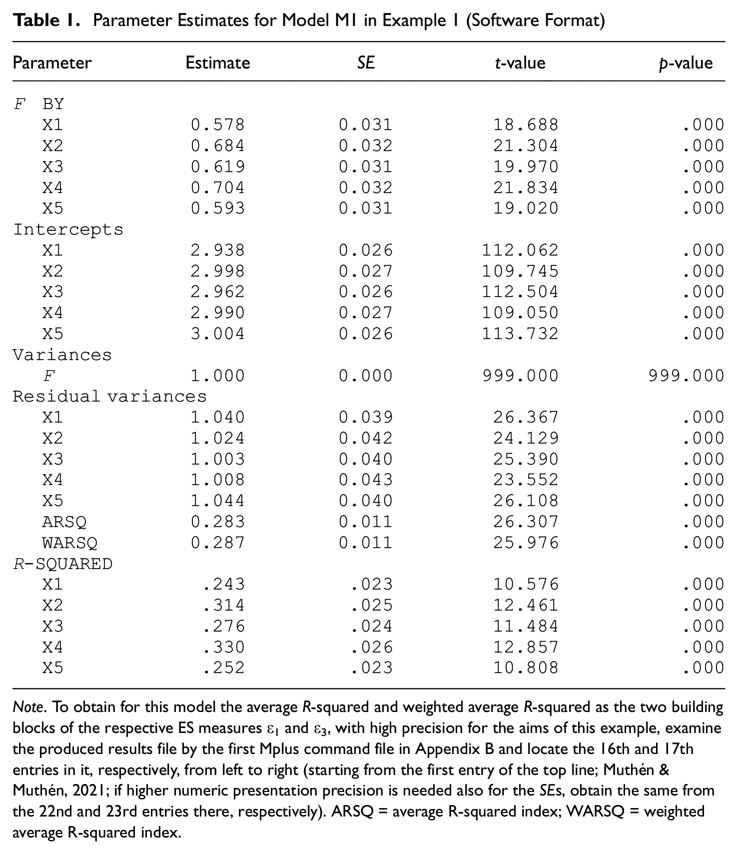
Note. To obtain for this model the average R-squared and weighted average R-squared as the two building blocks of the respective ES measures ε₁ and ε₃, with high precision for the aims of this example, examine the produced results file by the first Mplus command file in Appendix B and locate the 16th and 17th entries in it, respectively, from left to right (starting from the first entry of the top line; Muthén & Muthén, 2021; if higher numeric presentation precision is needed also for the SEs, obtain the same from the 22nd and 23rd entries there, respectively). ARSQ = average R-squared index; WARSQ = weighted average R-squared index.

Next, in this model, the first building blocks of the ES measures ε₁ and ε₃, namely, the average R-squared and weighted average R-squared for M1, are estimated as .282944 (.011) and .286965 (.011), respectively (standard errors given in parentheses; see Notes to Table 1 and Appendix B).⁴

In the second step, we fit the nested Model M2 to the same data and also obtain tenable fit indices: χ² = 16.263, df = 9, p = .062, and RMSEA = .020 (0, .035), similarly indicating a plausible model (with 90% confidence interval following RMSEA point estimate, as in the rest of this section). Table 2 presents the parameter estimates and indicator R-squared indices in M2, with their standard errors and associated statistics.

Table 2.

Parameter Estimates for Model M2 in Example 1 (Software Format)

Parameter	Estimate	SE	t-value	p-value
F BY
X1	0.634	0.015	41.252	.000
X2	0.634	0.015	41.252	.000
X3	0.634	0.015	41.252	.000
X4	0.634	0.015	41.252	.000
X5	0.634	0.015	41.252	.000
Intercepts
X1	2.938	0.027	110.518	.000
X2	2.998	0.027	111.019	.000
X3	2.962	0.026	112.007	.000
X4	2.990	0.027	110.785	.000
X5	3.004	0.027	112.673	.000
Variances
F	1.000	0.000	999.000	999.000
Residual variances
X1	1.011	0.037	27.293	.000
X2	1.056	0.039	27.420	.000
X3	0.996	0.037	27.204	.000
X4	1.054	0.038	27.396	.000
X5	1.020	0.037	27.327	.000
New/ additional parameters
ARSQ	0.282	0.011	26.045	.000
WARSQ	0.282	0.011	26.058	.000
R -SQUARED
X1	.285	.013	22.481	.000
X2	.276	.013	21.834	.000
X3	.288	.013	22.360	.000
X4	.276	.013	21.764	.000
X5	.283	.013	22.365	.000

Note. To obtain for this model the average R-squared and weighted average R-squared as the two building blocks of the respective ES measures ε₁ and ε₃, with higher precision for the aims of this example, examine the produced results file by the first Mplus command file in Appendix B and locate the 12th and 13th entries in it, respectively, from left to right (starting from the first entry of the top line; Muthén & Muthén, 2021; higher precision SEs, if needed, are found in the 17th and 18th entries in that file, respectively). ARSQ = average R-squared index; WARSQ = weighted average R-squared index.

In this model, the second building blocks of the ES measures ε₁ and ε₃, namely, the average R-squared and weighted average R-squared for M2, are estimated as .281508 (.011) and .281587 (.011), respectively (see Notes to Table 2 and Appendix B, and Note 4).

If one were to be willing to test the true score-equivalence restriction (10) using the LRT, the resulting test statistic of the loading constraint (10) would be equal to 16.263 – 3.497 = 12.766, for degrees of freedom = 9 – 5 = 4, and hence would be associated with a p-value of .012 (see also Note 5; for example, Bollen, 1989). Therefore, the LRT would reject the null hypothesis (10) (at the conventional significance level of .05). That is, despite the rather minor violation of the restriction (10) in the underlying population, as explicated earlier, the pertinent statistical test result would suggest in effect incorrectly the rejection of this parameter restraint. We stress, however, that constraint (10) is essentially fulfilled in the population (see preceding discussion). Hence, the present is an example of a spurious finding of parameter restriction rejection by the respective statistical test (LRT), which is mostly due to the large sample effect.

Instead of (or in addition to) conducting this statistical test of the restriction (10), we can proceed using the ES measures discussed in the article, which are applicable in this setting. With this in mind, as indicated in the preceding section, to facilitate their interval estimation we request first r = 2,000 bootstrap resamples with replacement that are saved separately for the following use. (See the second Mplus source code in Appendix B and its Notes.) In a next step, to each of these resamples we fit Model M1, and then Model M2, utilizing the external Monte Carlo facility in Mplus (Muthén & Muthén, 2021, Chapter 12). Thereby, we save the resulting parameter estimates per model and resample. (See the respective Mplus command files in Appendix C accomplishing this goal, and notice the use of the SAVEDATA command as well as the names of produced results data sets, each with 2,000 records.)

To illustrate next an application of the interval estimates of the aforementioned ES indices ε₁ and ε₃ (see also ε₂, with ε₃ being a special case of it that is of relevance here), we employ the Stata command file in Appendix D that yields their 95% bootstrap CIs (see also Note to that appendix and Note 4). Accordingly, this CI for ε₁ results as [.000515, .003641], and that for ε₃ as [.001797, .015698]. (See foregoing discussion in this section for their point estimates in the initially simulated data set, which are also of importance and fall within the respective CIs.) As each of these two CIs is located entirely above 0 and below .02, and thus covers only a rather limited range of very small numbers, it is suggested that the effect of the examined nesting constraint (10) is negligible. Therefore, this parameter restriction of loading equality can be treated as plausible in the underlying population. The latter interpretation is consistent with the previous discussion in this section, which indicated the degree of population violation of (10) as effectively ignorable. We emphasize that the last finding and interpretation differs from the result of the statistical nested model test conducted earlier, whereas the application of the ES measures of this article allowed us to conclude that in practical terms the five used measures X₁ through X₅ can be treated as true-score equivalent (e.g., McDonald, 1999).

Example 2

In this subsection, as a further development of the aforementioned discussion we present a more extreme instance of a serious failure of the statistical nested models’ testing approach (LRT), namely, in a setting with (a) a fairly large sample size that is not unusual in complex design and nationally representative studies, as well as (b) markedly smaller and in effect trivial violation of a parameter constraint. To this end, within the same data generation setup as that of Example 1, we use now a sample size of n = 7,000 cases and a practically nonexistent if at all meaningful violation of the factor loading equality constraint in Equation 10. Specifically, the data on the five single-factor indicators, X₁ through X₅, are generated here following this model (cf. Example 1):

\begin{matrix} X_{1} = 3 + . 69 η_{1} + δ_{1}, \\ X_{2} = 3 + . 71 η_{1} + δ_{2}, \\ X_{3} = 3 + . 70 η_{1} + δ_{3}, \\ X_{4} = 3 + . 71 η_{1} + δ_{4}, \\ X_{5} = 3 + . 69 η_{1} + δ_{5}, \end{matrix}

(11)

where η₁ is a standard normal variate and the residuals, δ₁ to δ₅, are independent standard normal variables. (See Note 2 to Appendix A regarding the details of the data simulation process.) Based on this information, one readily finds (see the foregoing in this section) that the maximal loading discrepancy from their average is .01, that is, 1% of the population latent variance, and can thus be considered trivial for most, if not all, practical purposes if at all meaningful or important.

When Model M1 is fitted to the simulated data set (i.e., the unrestricted, single-factor model, as defined in Equation 11 and discussion following them), its tenable fit indices are found to be as follows: χ² = 3.309, df = 5, p = .652, and RMSEA = 0 [0, .013]; see Appendix B). Similarly, Model M2 (i.e., the single-factor model with restriction [10] imposed on its five loadings) is associated with tenable fit indices as well: χ² = 14.612, df = 5, p = .102, and RMSEA = .009 [0, .018] (see Appendix B). Testing the nested Model M2 against M1 using the LRT, as stated in this section, yields a significant result: LRT statistic = 14.612 – 3.309 = 11.303, df = 4, p = .023.⁵ Tables 3 and 4 contain the parameter estimates and related statistics for Models M1 and M2 in this example.

Table 3.

Parameter Estimates for Model M1 in Example 2 (Software Format)

Parameter	Estimate	SE	t-value	p-value
F BY
X1	0.663	0.016	41.043	.000
X2	0.714	0.016	43.755	.000
X3	0.725	0.016	44.005	.000
X4	0.716	0.017	43.362	.000
X5	0.683	0.016	42.911	.000
Intercepts
X1	3.001	0.014	207.382	.000
X2	3.001	0.015	204.233	.000
X3	2.979	0.015	200.753	.000
X4	2.989	0.015	201.449	.000
X5	2.986	0.014	208.701	.000
Variances
F	1.000	0.000	999.000	999.000
Residual variances
X1	1.026	0.021	48.500	.000
X2	1.001	0.022	46.446	.000
X3	1.015	0.022	46.226	.000
X4	1.029	0.022	46.745	.000
X5	0.966	0.021	47.119	.000
New/additional parameters
ARSQ	0.328	0.006	55.835	.000
WARSQ	0.328	0.006	55.798	.000

Note. To obtain for this model the average R-squared and weighted average R-squared as the two building blocks of the respective ES measures ε₁ and ε₃, with higher precision for the aims of this example, examine the produced results file by the first Mplus command file in Appendix B and locate the 16th and 17th entries in it, respectively, from left to right (starting from the first entry of the top line; Muthén & Muthén, 2021; if higher numeric presentation precision is needed also for the SEs, obtain the same from the 22nd and 23rd entries there, respectively). ARSQ = average R-squared index; WARSQ = weighted average R-squared index.

Table 4.

Parameter Estimates for Model M1 in Example 2 (Software Format)

Parameter	Estimate	SE	t-value	p-value
F BY
X1	0.700	0.008	82.960	.000
X2	0.700	0.008	82.960	.000
X3	0.700	0.008	82.960	.000
X4	0.700	0.008	82.960	.000
X5	0.700	0.008	82.960	.000
Intercepts
X1	3.001	0.015	205.220	.000
X2	3.001	0.015	205.031	.000
X3	2.979	0.015	202.142	.000
X4	2.989	0.015	202.345	.000
X5	2.986	0.014	207.707	.000
Variances
F	1.000	0.000	999.000	999.000
Residual variances
X1	1.007	0.020	50.630	.000
X2	1.009	0.020	50.611	.000
X3	1.030	0.020	50.775	.000
X4	1.037	0.020	50.846	.000
X5	0.957	0.019	50.164	.000
New/additional parameters
ARSQ	0.327	0.006	55.738	.000
WARSQ	0.327	0.006	55.756	.000

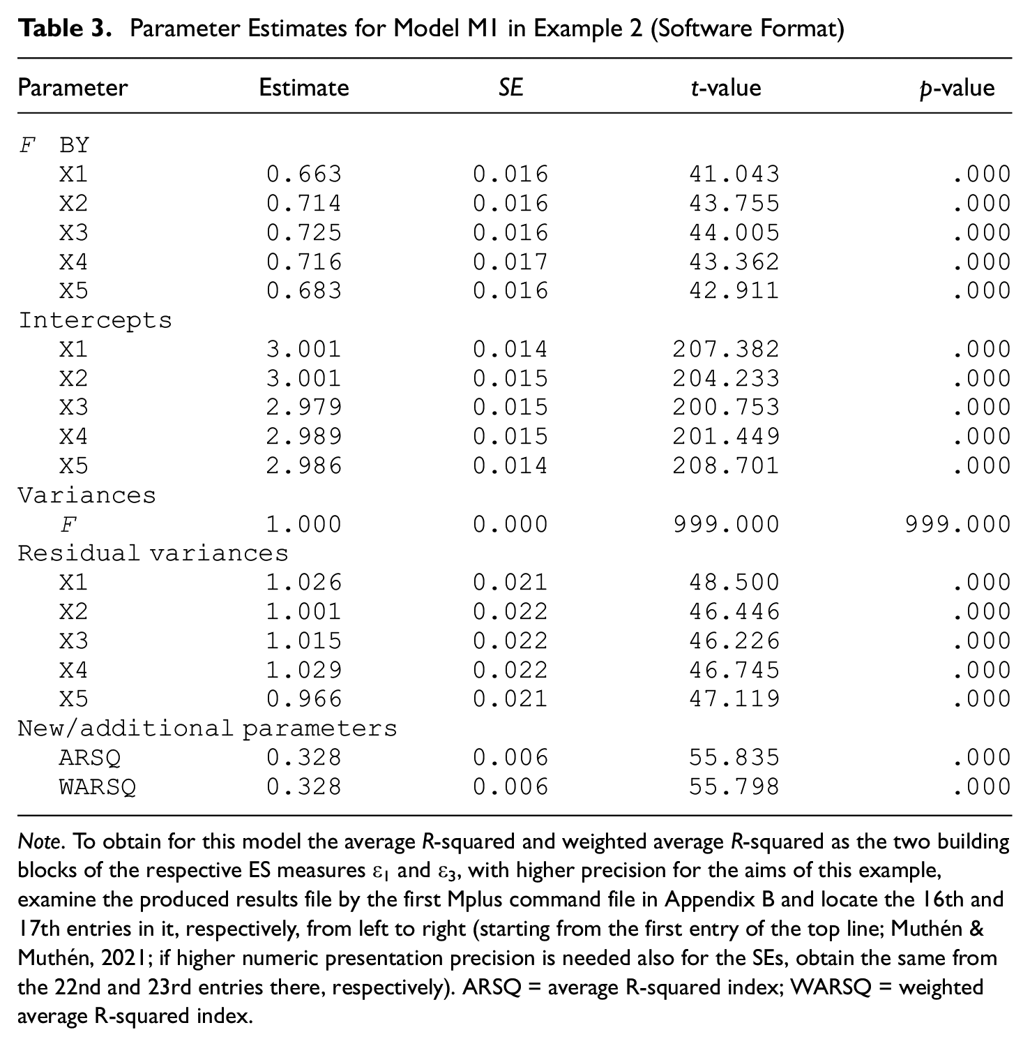
Note. To obtain for this model the average R-squared and weighted average R-squared as the two building blocks of the respective ES measures ε₁ and ε₃, with higher precision for the aims of this example, examine the produced results file by the first Mplus command file in Appendix B and locate the 16th and 17th entries in it, respectively, from left to right (starting from the first entry of the top line; Muthén & Muthén, 2021; if higher numeric presentation precision is needed also for the SEs, obtain the same from the 22nd and 23rd entries there, respectively). ARSQ = average R-squared index; WARSQ = weighted average R-squared index.

Following the earlier outlined procedure for estimation of the ES indices ε₁ and ε₃, we obtain their point estimates and 95% CIs correspondingly as follows: .000336 [.0001, .0008], and .000872 [.0002, .0028] (see Appendices C and D, Notes to Tables 3 and 4, Note 4, and the earlier discussion in this section).⁶ These ES indices clearly indicate effectively no impact of the constraints (10) on the local fit of the model, specifically in terms of the respective functions of the indicator R-squared indices, and hence that the constraint (10) can be considered not violated in the population to an extent that has practical importance. This conclusion is correct, given the specifics of the process of data simulation, and runs counter to the spuriously significant LRT result when testing constraint (10) as aforementioned.

Conclusion

This note discusses a class of ES measures whose aim is to aid educational, behavioral, and social scientists in their studies of nested CFA models. The measures represent important aspects of the cross-model discrepancies in the indicator R-squared indices, which result from imposing a studied parameter constraint in an initial CFA model. The described ES quantities do not involve explicitly sample size, and do not reflect statistical significance or lack thereof when testing the restriction under consideration (see also Note 3). With this feature, the ES measures are designed to be essentially resistant to the spurious effect of large sample size, when examining parameter restraints in CFA and more generally structural equation and latent variable models in empirical research.

The discussed ES indices and procedure for their evaluation possess several limitations. First, they represent some from possibly a (much) larger set of ES measures that could be devised as means for evaluating substantively meaningful aspects of the effects of nesting restrictions. We do not claim that the indices proposed are the best possible ES measures or that they are optimal in some sense, and certainly do not imply that they are the only ones possible to develop. We therefore encourage research into alternative ES measures and their comparison with the indices of this article. Second, there is some arbitrariness in the offered informal and tentative “guides” for interpretation of the point and interval estimates of these ES indices, which may also depend on the magnitude of the R-squared values of the observed variables in the initial model (denoted earlier as M1). For this reason, additional research is needed also on this issue, which we hope this article will stimulate, and resulting future studies will elaborate on (see also the following). Third, as mentioned in the introductory section, we assumed no clustering effects and a single-class (as opposed to mixture) population of concern. We conjecture that minor violations of the former assumption may not limit considerably the applicability, in a trustworthy way, of the described ES measures, except producing possibly shorter than warranted confidence intervals for them. The latter tendency may be counteracted to an acceptable degree by employing robust estimation methods (such as robust maximum likelihood when applicable). In this connection, we caution against using the ES indices of this article in mixture settings before appropriate modifications are carried out on the procedure of their application, to account for the multiplicity of latent classes. These modifications go beyond the confines of this note and are encouraged in future research. Fourth, the article does not intend to suggest or imply that the outlined ES evaluation method will always furnish ES point and interval estimates that are necessarily informative and straightforward to interpret in an unambiguous way. As indicated earlier, our only aim was to discuss such measures and offer them to empirical educational and behavioral scholars as a means potentially providing important additional and complementary information that may be useful in the process of examining nested CFA models. Fifth, and related to the preceding discussion, we stress that the proposed “guides” in relation to the interpretation of the ES indices obtained in an empirical study, are intended only to be initial proposals rather than meant to approach the status of “rules of thumb,” let alone “cutoffs” for such interpretation. In fact, the earlier discussion of the “guides” was not intended to offer anything beyond a rough idea as to what magnitude of the ES measures could be in our view meaningfully interpretable in educational and behavioral studies. We realize that this is an area that requires additional research, which goes beyond the confines of this article and is strongly encouraged. Sixth, we note that, in some settings, depending on the specifics of the imposed parameter constraint(s), it may be possible that some of the ES measures, as potentially complicated averages, are not sufficiently sensitive to the effect of imposing the constraint. In those cases, it may be likely, however, that some of the individual factor indicator R-squared indices could be more sensitive. These individual indices are obviously special cases of the ES measures of this article (see Equations 2 through 8 and Note 2) and thus their point and interval estimation can be readily obtained with the same procedure when appropriately adjusted to focus only on those individual indices. (Alternatively, see Raykov & Zajacova, 2012, for point and interval estimation of R-squared indices of observed variables and associated software-based procedure for latent variable models, which can then be directly applied.) Last but not least, we assumed that the indicators of the latent variables of concern were (approximately) continuous. We suspect that the discussed ES indices and their point and interval estimation procedure would be largely applicable in a trustworthy way also with indicators that take a relatively limited number of values in an empirical study, as long as they are at least 5 to 7 in number and preferably with relatively symmetric distributions (e.g., Rhemtulla et al., 2012). Extensions of the ES measures discussed in the article to the highly discrete items case, for instance, with binary or binary scored items or such with very few possible response values, seem to be feasible along similar lines (see Equations 2 through 8 and accompanying discussion), go beyond the confines of this article, and are encouraged to be developed in future research.

In conclusion, this article discusses ES measures that are (a) helpful in the potentially complicated process of evaluation of the effect of nesting constraints in CFA models, (b) free from an explicit relationship to sample size, and (c) unrelated to the outcome of the statistical test of the corresponding parameter restrictions. With this feature, these ES indices hold promise to aid educational and behavioral scientists using nested measurement models, particularly with large sample sizes, as is the case increasingly more often following the growing interest in large-scale and related studies in educational and psychological research.

Footnotes

Appendix A

Appendix B

Appendix C

Appendix D

Acknowledgements

The authors are grateful to S. Penev, T. Asparouhov, C. Huber, and L. K. Muthén for helpful discussions on bootstrap software applications. Thanks are also due to the Editor and two anonymous Referees for valuable comments and criticism on an earlier version of the article, which have contributed considerably to its improvement.

Declaration of Conflicting Interests

The authors declared no potential conflicts of interest with respect to the research, authorship, and/or publication of this article.

Funding

The authors received no financial support for the research, authorship, and/or publication of this article.

ORCID iDs

Tenko Raykov

Christine DiStefano

Notes

References

Agresti

(2002). Categorical data analysis. Wiley.

Bollen

K. A.

(1989). Structural equations with latent variables. Wiley.

Casella

Berger

J. O.

(2002). Statistical inference. Wadsworth.

Efron

B. J.

Tibshiriani

(1993). An introduction to the bootstrap. CRC Press.

Grissom

R. J.

Kim

J. J.

(2012). Effect sizes for research. Taylor & Francis.

Heeringa

West

B. T.

Berglund

(2017). Applied survey data analysis. CRC Press.

Jöreskog

K. G.

(1967). Some contributions to maximum likelihood factor analysis. Psychometrika, 32, 443–482.

Jöreskog

K. G.

(1971). Statistical analysis of sets of congeneric tests. Psychometrika, 36, 109–133.

Jöreskog

K. G.

Sörbom

(1996). LISREL8 user’s guide. Scientific Software International.

10.

McDonald

R. P.

(1999). Test theory. A unified treatment. Earlbaum.

11.

Millsap

R. E.

(2012). Statistical approaches to measurement invariance. Taylor & Francis.

12.

Mulaik

S. A.

(2009). Foundations of factor analysis. CRC Press.

13.

Muthén

L. K.

Muthén

B. O.

(2021). Mplus user’s guide. Muthén & Muthén.

14.

Raykov

Calvocoressi

(2021). Model selection and average proportion explained variance in exploratory factor analysis. Educational and Psychological Measurement, 81, 1203–1220.

15.

Raykov

DiStefano

(2021). Evaluating restrictive models in behavioral research: Local misfit overrides overall model plausibility. Educational and Psychological Measurement, 81, 980–995.

16.

Raykov

Marcoulides

G. A.

(2006). A first course in structural equation modeling. Earlbaum.

17.

Raykov

Marcoulides

G. A.

(2016). Scale reliability evaluation under multiple assumption violations. Structural Equation Modeling, 23, 302–313.

18.

Raykov

Marcoulides

G. A.

Chang

(2016). Studying population heterogeneity in finite mixture settings using latent variable modeling. Structural Equation Modeling, 23, 726–730.

19.

Raykov

Marcoulides

G. A.

Millsap

R. E.

(2013). Examining factorial invariance: A multiple testing procedure. Educational and Psychological Measurement, 73, 713–727.

20.

Raykov

Zajacova

(2012). On latent change model choice in longitudinal studies. Structural Equation Modeling, 19, 580–592.

21.

Rhemtulla

Brosseau-Liard

Savalei

(2012). When can categorical variables be treated as continuous? A comparison of robust continuous and categorical SEM estimation methods under suboptimal conditions. Psychological Methods, 18, 354–369.

22.

Schmidt

F. L.

(1996). Statistical significance testing and cumulative knowledge in psychology: Implications for training of researchers. Psychological Methods, 1, 115–129.

23.

Stata Base Reference Manual. (2019). Stata Press.