Investigating Confidence Intervals of Item Parameters When Some Item Parameters Take Priors in the 2PL and 3PL Models

Abstract

To reduce the chance of Heywood cases or nonconvergence in estimating the 2PL or the 3PL model in the marginal maximum likelihood with the expectation-maximization (MML-EM) estimation method, priors for the item slope parameter in the 2PL model or for the pseudo-guessing parameter in the 3PL model can be used and the marginal maximum a posteriori (MMAP) and posterior standard error (PSE) are estimated. Confidence intervals (CIs) for these parameters and other parameters which did not take any priors were investigated with popular prior distributions, different error covariance estimation methods, test lengths, and sample sizes. A seemingly paradoxical result was that, when priors were taken, the conditions of the error covariance estimation methods known to be better in the literature (Louis or Oakes method in this study) did not yield the best results for the CI performance, while the conditions of the cross-product method for the error covariance estimation which has the tendency of upward bias in estimating the standard errors exhibited better CI performance. Other important findings for the CI performance are also discussed.

Keywords

2PL model 3PL model confidence interval IRT Item priors priors for item parameters

Item response theory (IRT) is a widely used latent variable modeling method in educational and psychological measurement. Due to its versatility, IRT has been used for many applications such as test construction, differential item functioning, and test equating (de Ayala, 2009; Yen & Fitzpatrick, 2006). A major reason for IRT’s popularity was due to successful realizations of estimation methods for IRT models. For the item parameter estimation of IRT models, the marginal maximum likelihood (MML) method with the application of the expectation-maximization (EM) algorithm (Bock & Aitkin, 1981) and its variant where item parameters take priors in the context of the MML EM method (e.g., Mislevy & Stocking, 1989; Mislevy, 1986; Tsutakawa, 1992) are the most frequently used methods in research and practice.

When estimating an IRT model, the point estimates of model parameters are the first major interest (e.g., item difficult and item discrimination [or slope] parameter estimates). Uncertainty estimates such as confidence intervals (CIs) of model parameters, however, are important and may be of another interest in IRT applications because the interval estimates take into account sampling fluctuations, accommodating the extent of sampling variability in the point estimation. In estimating an IRT model with the MML method, the person ability parameters are assumed to take a certain distribution a priori (or simply stating that they are assumed to follow a distribution from the traditional frequentist point of view), such as normal distribution, while the item parameters do not take any prior distributions. In this “pure” MML approach, the item parameter estimates are the maximum likelihood (ML) estimates and their large-sample theory standard errors (SEs) are obtained typically from an observed or expected information matrix. The 100 ×(1 $- α$ )% CI for an item parameter, as an interval estimation in the MML approach, is computed as

\hat{ζ} \pm z_{α / 2} \hat{SE} (\hat{ζ})

(1)

where $\hat{ζ}$ = the item parameter estimate, $α$ = the nominal significance level (.05 in this study), and $z_{\frac{α}{2}}$ is the quantile that corresponds to $α / 2$ in the standard normal distribution. The probability statement attached to the above interval estimation is based on the approximate normality from the large-sample theory in ML.

In the MML estimation, typically no prior distributions are used for item parameters. However, when a sample size is small, or to prevent unreasonable estimates or nonconvergence, prior distributions for item parameters may be used in the estimation process. For example, an application of the 2-parameter logistic model (2PLM) may exhibit unreasonable item slope estimates (e.g., very large or extremely uncommon values) or nonconvergence for several items due to Heywood cases. Also, in applications of the 3-parameter logistic model (3PLM), it is common to find the use of prior distributions for the pseudo-guessing parameters to reduce the issue of nonconvergence due to the model complexity by adding the pseudo-guessing parameters. When the item prior distributions are used in the MML-EM approach, the estimation method may be called a marginalized Bayesian EM approach, where the point estimates of item parameters are the marginal maximum a posteriori (MMAP) and the SE of item parameter is replaced by the posterior standard error (PSE). MMAP and PSE are the terms adopted for the MML-EM approach. They are to differentiate from MAP and posterior standard deviation (PSD) from a posterior distribution in a Bayesian approach using Markov Chain and Monte Carlo (MCMC). In the Bayesian modeling with MCMC, a credibility (or posterior) interval, which is similar to CI can also be obtained directly from the simulated posterior distribution where the 100 $\times (1 - α / 2)$ th and 100 $\times α / 2$ th quantiles are located. MMAP and PSE are not obtained from the simulated posterior distributions. In the MML-EM and the marginalized Bayesian EM approach, only the point estimates of item parameters are obtained. MMAP may be viewed as a point estimate which maximizes a weighted likelihood that consists of the usual MML objective function and the prior part. A separate method to find SE or PSE is necessary in the MML-EM and the marginalized Bayesian EM approach. The SE or PSE are usually obtained from an observed information matrix. MMAP and PSE are the only available quantities for the end users when one adopts the marginalized Bayesian EM approach. A straightforward procedure in this occasion to obtain an interval estimate for an item parameter is to mimic the CI procedure in the MML estimation, that is

{\hat{ζ}}_{MMAP} \pm z_{α / 2} \hat{PSE}

(2)

This interval estimation may be treated as an approximation of the 95% CI in the marginalized Bayesian EM approach to formula (1). This CI construction assumes that $\hat{ζ} \approx {\hat{ζ}}_{MMAP}$ and $\hat{SE} (\hat{ξ}) \approx \hat{PSE}$ in a large sample. In finite samples whose sizes are not large, especially when item prior distributions are considered, given that the specified priors do not match the true population prior distributions in real data analysis, the above CI formula is unlikely to be a good approximation to the 95% CI because ${\hat{ζ}}_{MMAP}$ is a shrinkage estimator and $\hat{PSE}$ is less than $\hat{SE} (\hat{ξ})$ .

Popular IRT programs often uses MML-EM as default, providing the marginalized Bayesian EM approach as an option. When item priors are employed, practitioners end up with the point estimates of items parameters (MMAPs) and their PSEs, and are more likely to resort to formula (2) to construct an interval estimate and use it as 95% CI. This study investigates the performance of the interval estimation procedure, formula (2) as 95% CI for the 2PLM and the 3PLM applications when item priors are taken under the marginalized Bayesian EM estimation approach. Currently, the literature does not show the behavior of formula (2) in the marginalized Bayesian EM estimation context. The 2PLM estimation usually works well without item priors, but there exist some situations, especially in some small samples, which use priors for item slope parameters because of improper solutions or nonconvergence in the item slope parameter estimation. Therefore, the focus of our investigations is on the item slope parameters in the 2PLM estimation when taking priors. For the 3PLM applications, the investigation centers on the pseudo guessing parameters when taking priors, given the common practice of using priors for the pseudo guessing parameters. Also in this study, the distributions of item slope and pseudo-guessing parameters for data generation are not the same as the prior distributions for the item slope and the pseudo-guessing parameters in the 2PLM and 3PLM estimation. (More details on the item prior distributions are provided later in the “Method” section.) In real data analysis, it is highly likely that chosen prior distributions do not match the true unknown distributions of parameters exactly. Given this reality, the parameter simulation distributions were chosen not to be identical with the specified prior distributions for the item slope and the pseudo-guessing parameters. In this sense, this study is also a sensitivity analysis for using widely known prior distributions, examining the degree of robustness of them as well.

The term SE is used from now on to denote SE in the MML-EM or PSE for simplicity. Also, the interval estimation procedures (1) and (2) will be referred to as, simply, CI construction procedures although formula (2) may be more properly called as posterior CI. As mentioned, in the MML-EM and the marginalized Bayesian EM approach, an SE method is required separately. Because SEs play a pivotal role in the CI construction procedures, they are reviewed briefly in the next section.

Methods for Standard Error Estimation

The descriptions of SE methods here are brief. Readers interested in more detailed technical treatment of those are referred to the references in the descriptions later. SE values are computed by taking the square root of the diagonal elements in the error covariance matrix which is the inverse of an information matrix. Because the EM approach only yields a complete-data information matrix in the process of estimation as a byproduct, methods to estimate an observed information matrix (or error covariance matrix) have been proposed in the IRT literature. In the MML-EM estimation context, those include the “cross-product” method (Meilijson, 1989; Pawitan, 2001.), the supplemented EM algorithm (S-EM: Cai, 2008; Meng & Rubin, 1991), the sandwich covariance matrix (White, 1982; Yuan et al., 2014), the Oakes method (Chalmers, 2018; Oakes, 1999; Pritikin, 2017)), and the Louis method with a refined computational approach (Liu & Chalmers, 2020; Louis, 1982).¹ Of these, the most studied methods up to now appears to be S-EM and the cross-product, the latter of which tends to be included as part of the comparisons with other major SE method(s) in the studies due to its relative simplicity and computational efficiency. The performance of S-EM was investigated by Cai (2008), Tian et al. (2013), Paek and Cai (2014), Pritikin (2017), and Chalmers (2018). The performances of the sandwich covariance, the Oakes, and the Louis were not fully documented yet by many studies in the IRT literature. As far as the authors are aware, Yuan et al. (2014) is the only published study on the performance of the sandwich procedure in IRT. To formulate the sandwich estimator, Yuan et al. combined the cross-product method in the IRT literature and the Louis (1982) information form. For the Louis (1982) method, a refined computational approach was proposed by Liu and Chalmers (2021). Their approach greatly enhanced the computational efficiency of the Louis procedure, demonstrating the refined approach’s potential across IRT and other latent variable models.

With respect to finite difference methods to approximate the observed information matrix, the Oakes method with finite difference applications (Chalmers, 2018; Pritikin, 2017) has been shown to be as good as or better than S-EM. More concretely, Pritikin (2017) implemented the Oakes method with the forward difference numerical approximation, comparing it with three types of S-EM procedures: original S-EM by Meng and Rubin (1991), a refined S-EM by Tian et al. (2013), and another refined S-EM by Pritikin (2016). Chalmers (2018) used the three numerical approximation methods (forward, central, and Richardson’s extrapolation) for the Oakes procedure and compared them with the refined S-EM by Tian et al., concluding that the central difference or the Richardson extrapolation method worked best. The Oakes procedure with numerical approximation was preferred to S-EM by both Chalmers (2018) and Pritikin (2017) for its accuracy and computational efficiency (calculation speed and reducing the occasions of nonconvergence in the calculation of S-EM error covariance matrix). Three SE methods were included in this study: cross-product denoted as CRP, Louis, and Oakes.

As mentioned before, the CRP method is considered as the most straightforward computationally relative to the Louis and the Oakes method. It is the outer products of gradients. The Louis observed information procedure is more complex than the CRP involving the second-order partial derivative, but it could provide a better sample-based approximation of the information matrix than CRP (see Yuan et al., 2014). The Louis observed information can be expressed as two components and one of the two is equivalent to the CRP (Liu & Chalmers, 2020; Yuan et al., 2014). Under the correct model specification assumption, as sample size N increases, CRP and the Louis observed information matrices becomes equal, the CRP component in the Louis method approaching zero (Yuan et al., 2014). The Oakes method, as the S-EM method,² is built upon the missing information principle, that is, the observed information matrix ( $I_{o}$ ) is equal to the difference between the information matrix of the complete data ( $I_{c}$ ) and the information matrix of the missing data ( $I_{m}$ ) (Orchard & Woodbury, 1972). Chalmers (2018) showed that the Oakes method with two numerical approximations—both the central and the Richardson extrapolation methods—worked better than with the numerical approximation of the forward difference method, while the central method exhibited higher computational efficiency than the Richardson extrapolation method. The Oakes procedure with the central difference method was used in this study.

In the Oakes procedure, when items take priors, their first- and second-order derivatives (i.e., gradients and Hessian matrix) of the priors are added in the process of obtaining the complete data information and the missing data information to obtain the observed information. For the Louis procedure, Liu and Chalmers (2020) showed that its information, when item priors are used, is equal to the Louis information without item parameter prior plus the Hessian of the item parameter priors, that is, $I_{L}^{*} = I_{L} + H (ξ)$ where $I_{L}^{*}$ is the updated observed information for the Louis method with item parameter priors, $I_{L}$ is the right-hand side of Equation (7), and $H (ξ)$ is the Hessian matrix of the item parameter priors. Thus, the vector of the standard errors of item parameters for the Louis method with item parameter priors is the square root of ${diag [I^{*}]}^{- 1}$ . Under the standard regularity condition and the correct model specification assumption, with a large sample size, the information of the CRP with item parameter priors can also be expressed as the sum of the CRP information without item parameter priors and the Hessian of the item parameter priors.

Method

Simulations were conducted to assess the CI procedures, formula (1) in the MML-EM and formula (2) in the marginalized Bayesian EM approach.

IRT models used in this study are the unidimensional 2PLM and 3PLM. The 3PLM item response function is

P_{j} (θ_{i}) = g_{j} + (1 - g_{j}) \frac{\exp [a_{j} (θ_{i} - b_{j})]}{1 + \exp [a_{j} (θ_{i} - b_{j})]},

(3)

where $θ_{i}$ is the ith person ability or latent trait score $(i = 1, 2, \dots, N)$ , $a_{j}$ is the jth item slope or discrimination parameter $(j = 1, 2, \dots, L)$ , $b_{j}$ is the jth item difficulty parameter, and $g_{j}$ is the $j$ th item pseudo-guessing parameter. In the MML-EM and the marginalized Bayesian EM approach, $θ$ is assumed to follow a certain distribution $h (θ)$ , which was a normal distribution (with its mean equal to zero and its standard deviation [SD] equal to one for the model identification purpose) in this study. The 2PLM is obtained when $g_{j}$ = 0.

The item response data were generated following the standard IRT data generation method. The steps to generate item response data are as follows. For a response to the jth item by the ith person, (a) compute $P$ —probability of a correct answer with the data generating item and parson parameters. (See the “Parameter Value for Data Generation in the Method section for the details of drawing the item and person parameters); (b) draw a value, $u$ , from the standard uniform distribution; (c) assign 1 if $u < P$ and assign 0, otherwise.

The simulation factors were SE methods, sample sizes, test lengths, and prior distributions for item slope parameters in the 2PLM and for the pseudo guessing parameters in the 3PLM. CIs were constructed by fitting correct models with and without item priors (i.e., 2PLM fit to 2PLM data and 3PLM fit to 3PLM data). The number of replications per condition was 1000. Data simulation and IRT model estimation with different SE methods under the MML-EM and the marginalized Bayesian EM approach where item priors are taken, were implemented using the “mirt” package (Chalmers, 2012) in the R statistical language and environment for statistical computing (R Core Team, 2020).³ Convergence was checked using the default check provided by the “mirt” program and its second-order test of a unique modal solution. In addition, unreasonable or improper solutions were flagged if $a_{j} \in [0, 10), b_{j} \in (- 10, 10)$ , and $g_{j} \in (0, 1)$ were not met for both prior and no-prior conditions and if any of the standard error estimates were greater than 2.5. Under these checking rules, the rates for the valid data sets for the 2PLM ranged from .949 to 1. For the 3PLM, they were between .961 and 1. When a replication turns out to be flagged by these rules, it was discarded and the simulation of the replications was carried on to reach the 1000 replications, all of which pass the above checks.

SE Methods

As mentioned in the section of “Methods for Standard Error Estimation,” cross-product denoted as CRP, Louis, and Oakes methods were included in this study. CRP is computationally most straightforward and used as a default method in some IRT programs (e.g., IRTPRO by Vector Psychometric Group, LLC., 2021). The Louis method appeared to regain attention recently as an SE method in IRT (Liu & Chalmers, 2020) although its performance is not yet completely and fully documented yet (for scenarios where item parameter takes its prior as in this study).⁴ Past studies (Chalmers, 2018; Pritikin, 2017) indicated Oakes performed the same or better than S-EM. The Oakes method is a default method in the “mirt” program. Note that although the three SE methods were originally included, the results showed that the Oakes and the Louis produced virtually the same results, therefore, in the presentation of the results, the Louis method is omitted.

Test Length

When data followed the 2PLM, a 20-item test and a 40-item test were simulated. Given that the 3PLM is popular in large-scale educational achievement testing which tends to have a relatively long test, 30-item and 50-item tests were simulated for the 3PLM data.

Sample Size

In the 2PLM data, sample sizes of 200, 900, and 1600 were used. The sample sizes for the 3PLM data were 1000, 1700, and 2400. Some small-scale preliminary analyses were conducted with smaller sample sizes (e.g., less than 200 for the 2PLM and 1000 for the 3PLM). Based on some preliminary analysis, large sample sizes (900 or 1600 for the 2PLM application and 1700 or 2400 for the 3PLM) were selected to examine the extent of the improvement in the approximation of the CR procedure, formula (2).

Prior Distributions for Item Parameters

When the 2PLM was fitted to the 2PLM data, the item slope parameters ( $a_{j}$ ) took their prior distributions. For the item slope parameters, the use of lognormal distributions is popular in research and practice. (The manual of the BILOG-MG program [Scientific Software International, Inc., 2003] shows the use of logN(0, 0.5)). Two lognormal distributions were used as priors for the item slope parameters in the 2PLM estimation: $a_{j} ~ lognormal (0, 0.5)$ denoted by logN(0, 0.5) and $a_{j} ~ lognormal (0, 1)$ denoted by logN(0, 1) where each of the two numbers in the parentheses represents mean and SD, respectively. The latter, logN(0, 1), is a weaker prior than the former in that it has a larger SD. In addition, a no-prior condition where the slope parameter does not take a prior distribution was included. In the 2PLM model estimation, across the two lognormal and no-prior conditions, the item difficulty parameters did not take prior distributions. Graphical presentations of the prior distributions for the slope parameters are shown in Figure 1 (the plots of the first row) and descriptive statistics for the prior distribution are presented in the top panel under “Prior distribution” in Table 1.

Figure 1.

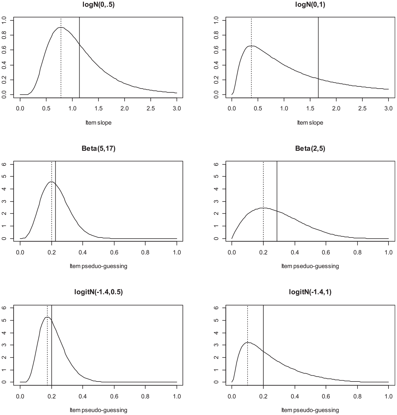
Prior Distributions For Item Slope and Pseudo Guessing Parameters

Table 1.

Descriptive Statistics for Prior Distributions and for Parameter Simulation Distributions.

	Prior distribution	E(X)	SD	Mode
2PLM slope parameter	lognormal(0, 0.5)	1.13	0.60	0.78
	lognormal(0, 1)	1.65	2.16	0.37
3PLM pseudo-guessing parameter	beta(5, 17)	0.23	0.09	0.20
	beta(2, 5)	0.29	0.16	0.20
	logitnormal(–1.4, 0.5)	0.20	0.08	0.17
	logitnormal(–1.4, 1)	0.20	0.16	0.10
Parameter simulation distribution
2PLM slope parameter	truncated-lognormal(.25, .25) with lower limit = .7 and upper limit = 3	1.33	0.33	1.21
3PLM pseudo-guessing parameter	uniform(0.05, 0.3)	0.18	0.07	Any value on (0.05, 3)

Note. 2PLM = 2-parameter logistic model; 3PLM = 3-parameter logistic model.

Prior distributions of the slope parameters are positively skewed. LogN(0, 1) is flatter than logN(0, 0.5) and the difference between the mean (solid line) and the mode (dotted line) is larger in the logN(0, 1) than logN(0, 0.5). The expectation E(X), the SD, and the mode of $a_{j}$ for logN( $0, 0.5)$ are 1.13, 0.60, and 0.78, respectively. For logN(0, 1), they are 1.65, 2.16, and 0.37, respectively. In terms of the mode, logN(0, 1) is farther away than logN(0, 0.5) from the parameter simulation distribution (, which is described below), while logN(0, 1) exhibits the wider spread (i.e., the largest SD) than logN(0, 0.5).

In the 3PLM fit to the 3PLM data, four types of prior distributions were used for the pseudo-guessing parameters ( $g_{j}$ ) while the slope and the difficulty parameters did not take prior distributions. Two beta distributions and two logitnormal distributions were used for $g_{j}$ : $g_{j} ~ Beta (5, 17)$ denoted by B(5, 17) and d $g_{j} ~ Beta (2, 5)$ denoted by B(2, 5), $g_{j} ~ logitnormal (- 1.4, 0.5)$ denoted by logitN(–1.4, 0.5), and $g_{j} ~ logitnormal (- 1.4, 1)$ denoted by logitN(–1.4, 1). Using the logitnormal distribution, $logit (g_{j}) = \log [g_{j} / (1 - g_{j})]$ is assumed to follow a normal distribution. The expectations of $g_{j}$ following B(5, 17) and B(2, 5) are 0.23 and 0.29. Their modes are the same as 0.2 which is closer to the expectation of the parameter simulation distribution. For the logitnomral distributions, their expectations are the same as 0.2 while their modes are different (0.17 and .1). The SDs of the two beta prior distributions are 0.09 and 0.16, respectively. The logitnormal priors’SDs were 0.08 and 0.16. Due to the lack of closed form solutions for the expectation and the SD of the logitnormal distributions, they were obtained by the delta method. Regarding SD, within each of the beta and the logitnormal distributions, SDs of the weak priors—B(2, 5) and logitN(–1.4, 1)—are approximately twice as large as those of the relatively strong prior distribution which are B(5, 17) and logitN(–1.4, 0.5). The third and the fourth row of Figure 1 show the shapes of the prior distributions for $g_{j}$ . It is clear that Beta(2, 5) and logitN(–1.4, 1) are flatter than their corresponding strong priors which have smaller SDs. Also, the difference between the expectation and the mode is larger in the relatively weak prior distributions. The use of B $(5, 17)$ is shown in some IRT programs such as BILOG-MG (Scientific Software International, Inc., 2003) and B(2, 5) was addressed for the 3PLM calibration in the flexMIRT program manual (Houts & Cai, 2020).⁵ LogitN(−1.4, 0.5) is very similar to logitN(−1.39, 0.5) which is also shown for a 3PLM calibration in the flexMIRT program manual. The last logitN(−1.4, 1) is observed sometimes in practice in large-scale assessment programs (Florida Department of Education, 2019).

Parameter Values for Data Generation

For both 2PLM and 3PLM, the item slope parameters ( $a_{j}$ ) and the item difficulty parameters $(b_{j}$ ) were drawn from truncated-lognormal and truncated-normal distributions, respectively. $a_{j}$ was drawn from a truncated-lognormal distribution where the mean is .25, the SD is .25, the lower limit is .7, and the upper limit is 3. $b_{j}$ was drawn from a truncated normal distribution with its mean equal to 0, its SD equal to 1, its lower limit equal to −2 and its upper limit equal to 2. For the pseudo guessing parameters ( $g_{j}$ ), they were drawn from a uniform distribution whose end points were .05 and .3.

Note again that, for the reason explained in the introduction, the prior distributions for the item slope and the pseudo-guessing parameters are not the same as those of item slope and pseudo-guessing parameters for data generation. (See the bottom panel in Table 1.)

Evaluation of CIs

For quantifying the performance of a CI procedure, coverage rate (CR) was used as outcome. CR is defined as

CR = \frac{\sum_{r} 1 (τ \in C I_{r})}{R}

(4)

where $τ$ is a true parameter of interest (e.g., a slope parameter), $C I_{r}$ is the CI for the rth replication data set ( $r = 1, 2, \dots, R = 1000$ ), and $1 (\cdot)$ is an indicator function (1 if $τ \in C I_{R}$ or 0 otherwise). CR was compared with $1 - α$ . Assuming that formula (2) provides a $100 \times (1 - α)$ CI, CR should be close to .95.

Results

The results from the Oakes SE method were virtually the same as those from the Louis SE method. The description of the results below, therefore, does not include the Louis SE method. Readers should be aware that the Louis SE method is always implied whenever the Oakes SE method is addressed. For those who are also interested in the item parameter recovery and the standard error estimation performance, their summaries are available upon request.

2PLM Data

In fitting the 2PLM to data, the slope parameters took lognormal(0, 0.5), lognormal(0, 1) or no prior distribution, while the item difficulty did not take any priors. Figure 2 provides CR for the slope parameters.

Figure 2.

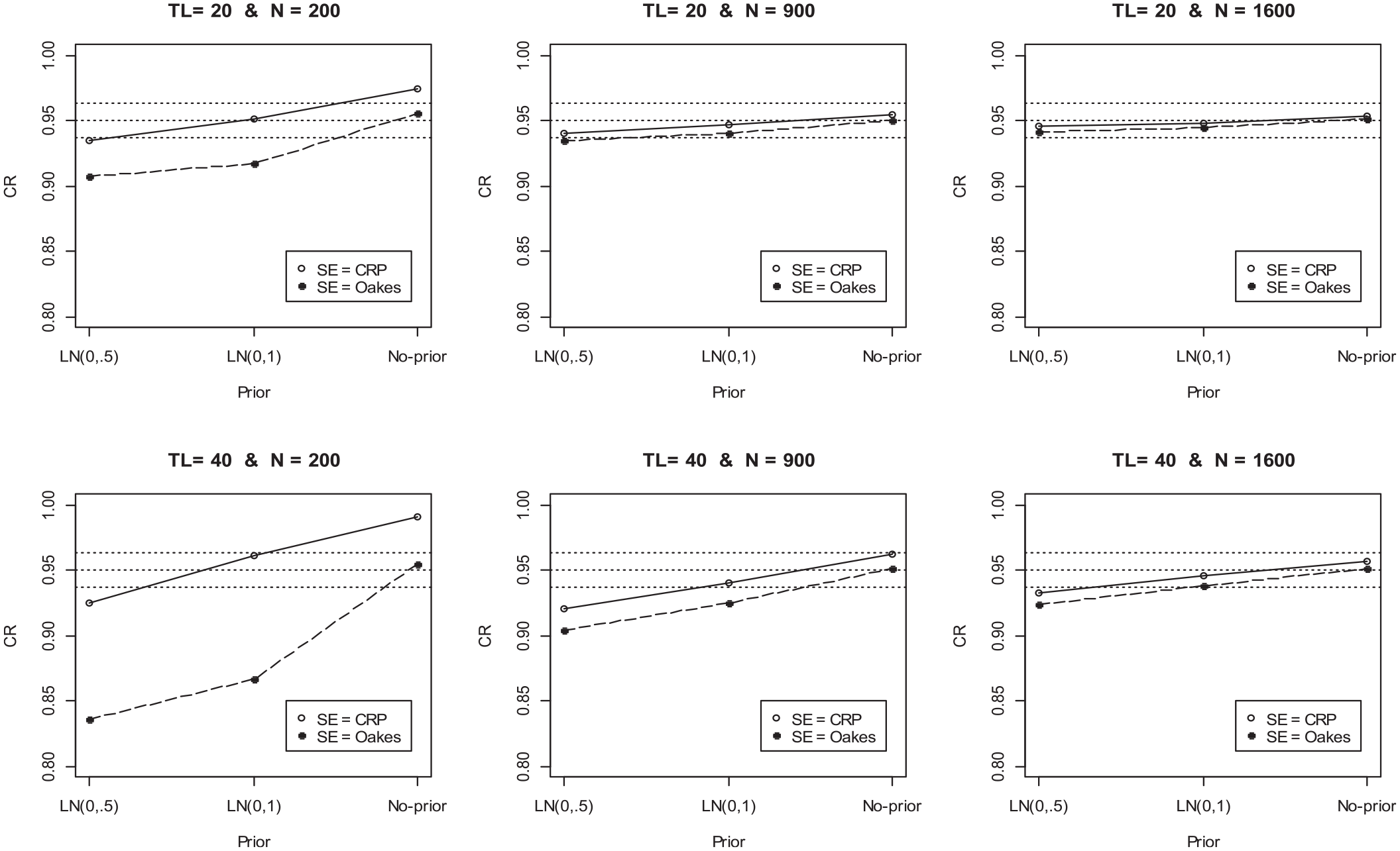
CR for the Item Slope Parameter (With Its Prior) in the 2PLM.

A larger sample size (N = 900 or 1600) increased the performance of CR, reducing bias (the deviation from .95). A short test, TL (test length) = 20, produced better performance of CR than a long test (TL = 40). The differences made by the SE methods and the prior distributions decreased in a larger sample and in a shorter test. The CRP SE method always produced larger CR than the Oakes SE method. When no prior is taken, the overestimation of CR in the CRP SE method is clearly noticed compared to the CR of the Oakes method. This is consistent with the past result that CRP tends to overestimate SE (Paek & Cai, 2014). Between the two prior conditions, the lognormal(0, 1) prior condition produced better CR performance than the lognormal(0, 0.5).

The percent bias of CR ( = $100 \times CR - 95{\rm %})$ is provided in Table 2. The conditions where CR deviates from the expected margin of error for .95 (upper and the lower dotted lines in the plots) under $α = . 05$ were highlighted in gray and their percent bias values are also highlighted in bold numbers in Table 2.

Table 2.

Percent Bias of CR for the Item Slope Parameter in the 2PLM.

TL	N	CRP			Oakes
		LN(0, 0.5)	LN(0, 1)	No-prior	LN(0, 0.5)	LN(0, 1)	No-prior (%)
	200	−1.5%	0.1%	2.4%	−4.3%	−3.3%	0.6
20	900	−0.9%	−0.3%	0.5%	−1.6%	−1.0%	0.0
	1600	−0.5%	−0.2%	0.3%	−0.9%	−0.5%	0.1
	200	−2.5%	1.2%	4.1%	−11.5%	−8.3%	0.5
40	900	−2.9%	−0.9%	1.2%	−4.6%	−2.5%	0.1
	1600	−1.7%	−0.4%	0.7%	−2.6%	−1.2%	0.2

Note. CR = coverage rate; 2PLM = 2-parameter logistic model; TL = test length.

Comparing the no-prior conditions of the two SE methods, the percent bias is larger in the CRP than the Oakes. Across all test lengths and sample sizes except for N = 1600 and TL = 20, the Oakes method with logN(0, 0.5) produced the largest size of bias, that is, the largest underestimation of CR, entailing significant sizes of bias. The logN(0, 0.5) prior condition, when combined with TL = 40, showed bias significantly deviating from .95 across all sample sizes. The logN(0, 1) prior condition yielded three cases of significant underestimation of CR with the Oakes SE method across all combinations of TL and N, while yielding none with the CRP SE method. The top four largest underestimation of CR (by −11.5% to −4.3%, which means CR = 83.5% to 90.7%) were found when the Oakes SE method was used with the lognormal prior distribution. The largest underestimation of CR was observed when a test was large (TL = 40), the sample size was small (N = 200), and the Oakes SE method was used with the logN(0, 0.5) prior distribution. Although the Oakes SE method is a better performer for the SE estimation than the CRP, as shown in the literature, the performance of the CI construction by formula (2) with the Oakes seems to suffer when item priors are used together. On the contrast, the overestimation tendency of SE in CRP appears to help with the performance of CR when the item prior distributions are used.

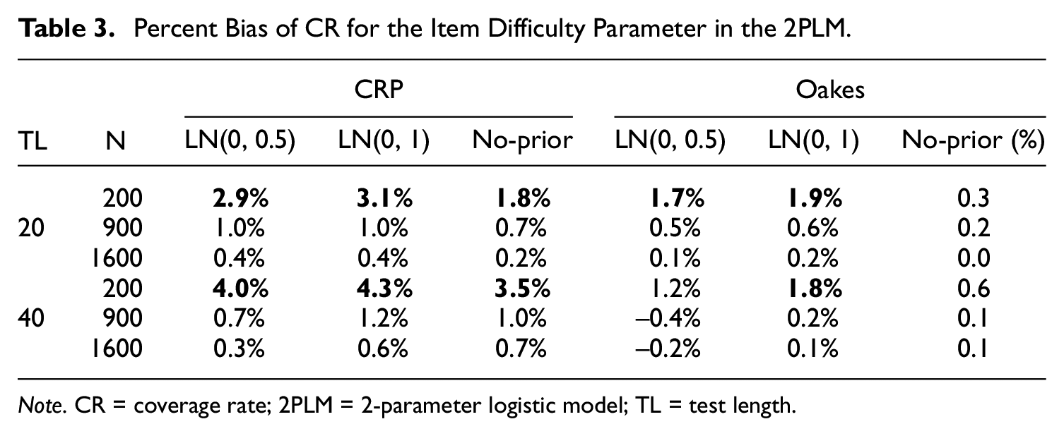
To check if there was any impact of the item slope priors on the CR of the item difficulty parameter which did not take any priors, the CR of the item difficulty parameters was examined. The CR for the item difficulty performed well in general, showing it is within the margin of error except for the small sample size of N = 200. The plot of CR and the percent bias of CR are shown in Figure 3 and Table 3.

Figure 3.

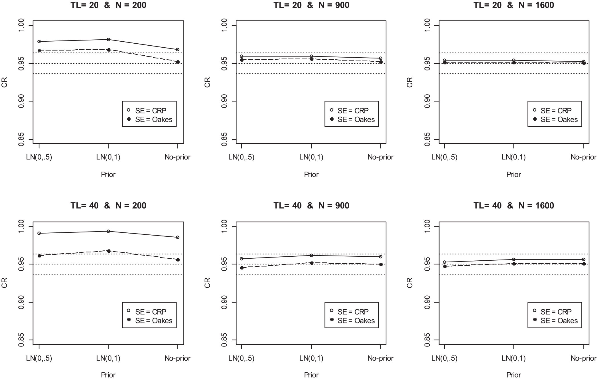
CR for the Item Difficulty Parameter (With No Prior) in the 2PLM.

Table 3.

Percent Bias of CR for the Item Difficulty Parameter in the 2PLM.

TL	N	CRP			Oakes
		LN(0, 0.5)	LN(0, 1)	No-prior	LN(0, 0.5)	LN(0, 1)	No-prior (%)
	200	2.9%	3.1%	1.8%	1.7%	1.9%	0.3
20	900	1.0%	1.0%	0.7%	0.5%	0.6%	0.2
	1600	0.4%	0.4%	0.2%	0.1%	0.2%	0.0
	200	4.0%	4.3%	3.5%	1.2%	1.8%	0.6
40	900	0.7%	1.2%	1.0%	−0.4%	0.2%	0.1
	1600	0.3%	0.6%	0.7%	−0.2%	0.1%	0.1

Note. CR = coverage rate; 2PLM = 2-parameter logistic model; TL = test length.

Note again, the item difficulty did not take any priors. CR and the percent bias in Figure 3 and Table 3 are presented in each of the simulation conditions for the item slope parameters. (For example, logN(0, 0.5) on the x-axis (denoted as LN(0, 0.5)) does not mean that the item difficulty took the lognormal prior distribution.). The same pattern of the relatively higher CR for the CRP than the Oakes SE method was observed. The differences between CRP and Oakes decreased as the sample size increases and the test length decreases, which were observed in the item slope parameter case. When the sample size is N = 200, the range of the overestimation of CR in CRP was from 1.7% to 3.1%, meaning CR ranged from 96.7% to 98.1%. This overestimation bias of CR for item difficulty parameters in CRP is again compatible with the past report of the overestimation tendency of CRP in the literature. The item difficulty parameters did not take priors and the CR of the item difficulty with the Oakes method performed better than the CRP method. Overall, in the 2PLM estimation, the impact of the item slope priors on the CI of the item difficulty appears to be little except for a relatively small sample size (N = 200).

3PLM Data

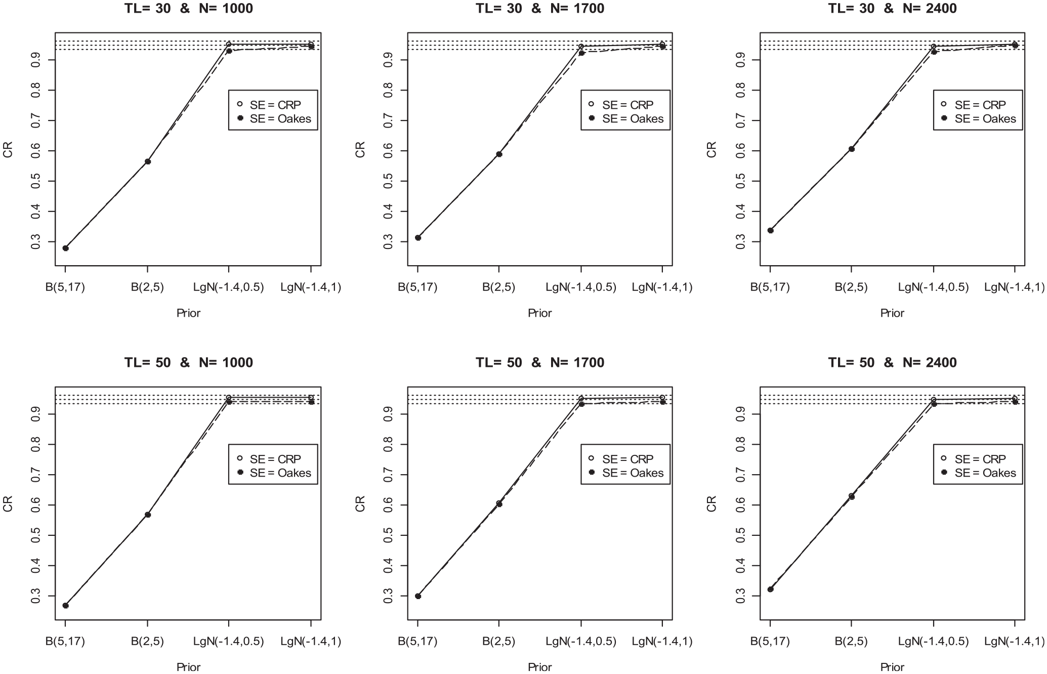
In the estimation of the 3PLM, the pseudo-guessing parameter ( $g_{j}$ ) took four different priors: $g_{j} ~$ B(5, 17), $g_{j}$ ~B(2, 5), $g_{j} ~$ logitN(–1.4, 0.5), and $g_{j} ~$ logitN(−1.4, 1). The means of the priors were .23, .29, .2, and .2, respectively, while their SDs were .09, .16, .08, and .16. Their modes were, .2, .2, .17, and .1, respectively. The other item parameters (item slope and difficulty) did not take any priors. Figure 4 and Table 4 show the CR plots and the percent bias of CR for the pseudo-guessing parameter.

Figure 4.

CR for the Pseudo-Guessing Parameter (With Its Prior) in the 3PLM.

Table 4.

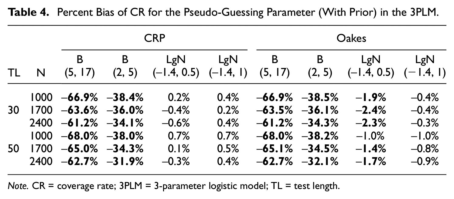
Percent Bias of CR for the Pseudo-Guessing Parameter (With Prior) in the 3PLM.

TL	N	CRP				Oakes
TL	N	B(5, 17)	B(2, 5)	LgN(–1.4, 0.5)	LgN(–1.4, 1)	B(5, 17)	B(2, 5)	LgN(–1.4, 0.5)	LgN(−1.4, 1)
	1000	−66.9%	−38.4%	0.2%	0.4%	−66.9%	−38.5%	−1.9%	−0.4%
30	1700	−63.6%	−36.0%	−0.4%	0.2%	−63.5%	−36.1%	−2.4%	−0.4%
	2400	−61.2%	−34.1%	−0.6%	0.4%	−61.2%	−34.3%	−2.3%	−0.3%
	1000	−68.0%	−38.0%	0.7%	0.7%	−68.0%	−38.2%	−1.0%	−1.0%
50	1700	−65.0%	−34.3%	0.1%	0.5%	−65.1%	−34.5%	−1.4%	−0.8%
	2400	−62.7%	−31.9%	−0.3%	0.4%	−62.7%	−32.1%	−1.7%	−0.9%

Note. CR = coverage rate; 3PLM = 3-parameter logistic model; TL = test length.

The impacts of TL and N were not consistent across different prior conditions. For the two beta prior distributions, increasing N reduced CR underestimation, but that was not always the case in the logitnormal prior conditions. The SE method showed the similar pattern as in the 2PLM. The CRP SE method tended to produce a larger CR than the Oakes method. In both the logitN(–1.4, 0.5) and logitN(–1.4, 1) prior conditions, the CR bias of the CRP SE methods were all within the margin of error. The magnitudes of the CR bias for the Oakes SE method were within the margin of error in the logitN(–1.4, 1) prior condition only. The use of the beta priors resulted in very large underestimation of CR while the logitnormal priors yielded much improved results. When logitN(–1.4, 0.5) was used with the Oakes SE method, the CRs were slightly off from the margin of error, especially when TL = 50 and N = 1700 and 2400, whose CRs were .936 (–1.4% bias) and .933 (−1.7% bias).

The CR and the percent bias of the item slope parameter which did not take any priors are shown in Figure 5 and Table 5.

Figure 5.

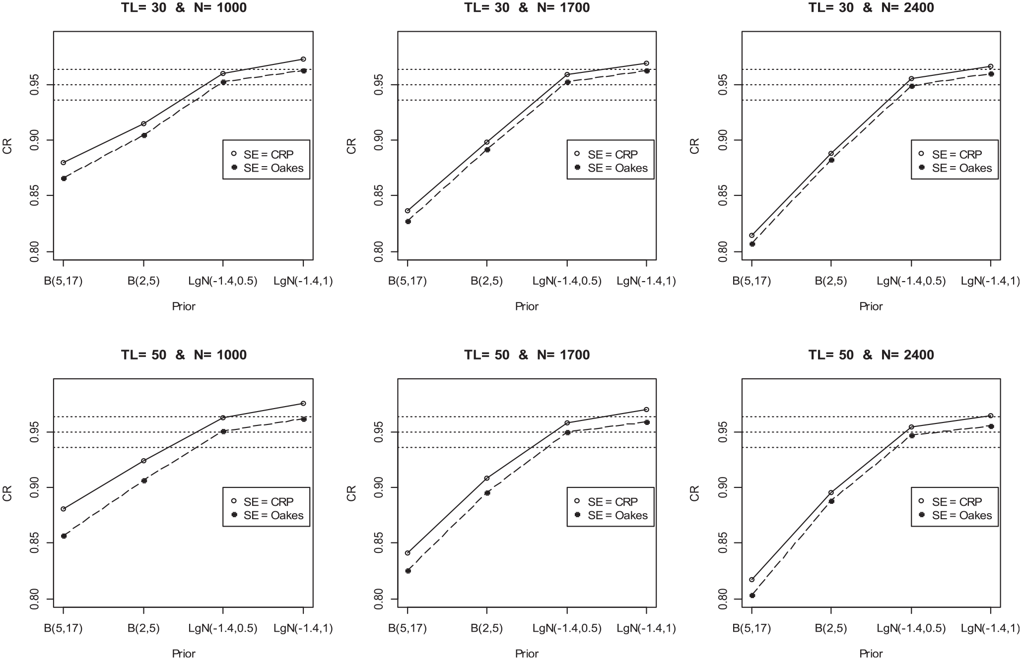
CR for the Item Slope Parameter (With No Prior) in the 3PLM.

Table 5.

Percent Bias of CR for the Item Slope Parameter (Without Prior) in the 3PLM.

TL	N	CRP				Oakes
		B(5, 17)	B(2, 5)	LgN(−1.4, 0.5)	LgN(−1.4, 1)	B(5, 17)	B(2, 5)	LgN(−1.4, 0.5)	LgN(−1.4, 1)
	1000	−7.0%	–3.5%	1.1%	2.4%	–8.4%	–4.5%	0.3%	1.3%
30	1700	–11.4%	–5.2%	0.9%	2.0%	–12.3%	–5.8%	0.2%	1.3%
	2400	–13.6%	–6.2%	0.5%	1.7%	–14.3%	–6.7%	–0.1%	1.0%
	1000	–6.9%	–2.6%	1.3%	2.6%	–9.4%	–4.3%	0.1%	1.2%
50	1700	–10.9%	–4.2%	0.8%	2.0%	–12.5%	–5.4%	0.0%	1.0%
	2400	–13.3%	–5.5%	0.5%	1.5%	−14.7%	−6.2%	−0.3%	0.6%

Note. CR = coverage rate; 3PLM = 3-parameter logistic model; TL = test length.

In the conditions where the pseudo guessing parameter took the beta priors, the CR of the item slope parameter showed very large underestimation of CR (by min = 2.6% and max = 13.6% underestimation), falling outside of the margin of error. As before, the CRP SE method condition produced higher CR than the Oakes CR. The impact of the overestimation tendency of the CRP SE method on CR was also observed in the logitN(–1.4, 1) prior condition, making the CR fall outside the margin of error. The CR of Oakes SE method conditions fell within the margin of error for both logitN(–1.4, 0.5) and logitN(–1.4, 0.5) prior conditions. No uniformly consistent pattern of CR bias was observed across all levels of N and TL. The differences between the CRP and the Oakes SE method conditions were smaller in TL = 30 than TL = 40. The average difference of the percent CR (= 100 × CR) between CRP and Oakes SE methods was 0.8% (min = 0.6% and max =1.4%) in TL = 30% and 1.3% (min = 0.7% and max = 1.7%) in TL = 50.

For the item difficulty parameter which did not take any priors, Figure 6 and Table 6 show the CR and the percent bias.

Figure 6.

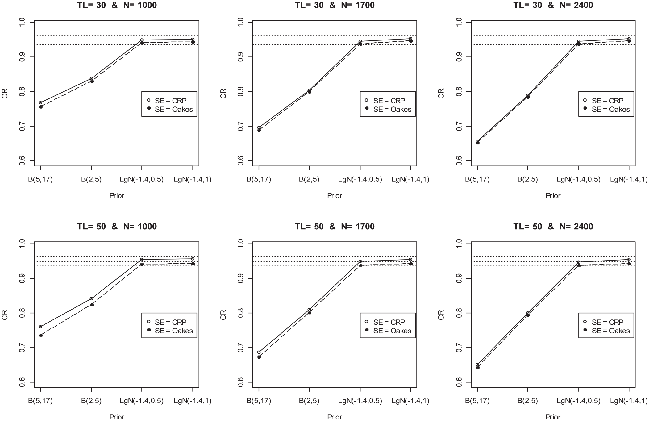
CR for the Item Difficulty Parameter (With No Prior) in the 3PLM.

Table 6.

Percent Bias of CR for the Item Difficulty Parameter (Without Prior) in the 3PLM.

TL	N	CRP				Oakes
		B(5, 17)	B(2, 5)	LgN(−1.4, 0.5)	LgN(−1.4, 1)	B(5, 17)	B(2, 5)	LgN(−1.4, 0.5)	LgN(−1.4, 1)
	1000	−18.2%	−11.1%	0.0%	0.2%	−19.4%	−12.0%	−0.8%	−0.5%
30	1700	−25.5%	−14.6%	−0.4%	0.4%	−26.1%	−15.1%	−1.1%	−0.2%
	2400	−29.4%	−16.2%	−0.5%	0.3%	−29.7%	−16.4%	−1.3%	−0.2%
	1000	−19.0%	−10.8%	0.5%	0.7%	−21.4%	−12.5%	−0.8%	−0.7%
50	1700	−26.4%	−14.0%	−0.1%	0.5%	−27.7%	−14.8%	−1.3%	−0.6%
	2400	−30.0%	−15.0%	−0.3%	0.4%	−30.8%	−15.5%	−1.2%	−0.6%

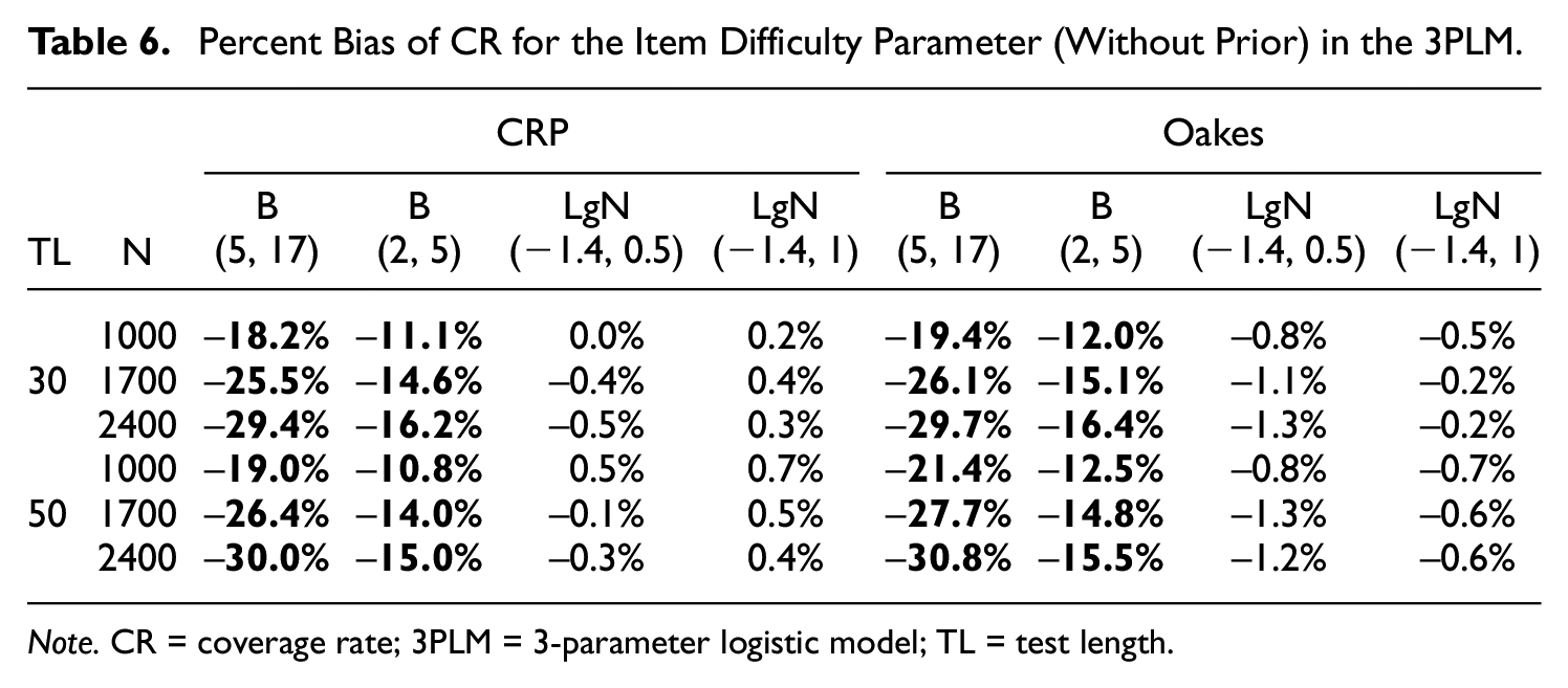
Note. CR = coverage rate; 3PLM = 3-parameter logistic model; TL = test length.

Overall, the patterns of the CR bias followed those of the item slope parameter which were mentioned above. The biggest impact factor was the prior distribution of the pseudo-guessing parameter as before. In the conditions where the beta priors were taken for the pseudo-guessing parameter, CR of item difficulty was underestimated to a very large extent and its percent bias ran the gamut from −11.1% to −30%. When the pseudo-guessing parameter took either logitN(–1.4, 0.5) and logitN(–1.4, 1) priors, all the CRs of item difficulty in both CRP and Oakes SE method conditions fell within the margin of error, though the tendency of the higher CR in the CRP than in the Oakes SE method was consistently observed as in all other parameter CIs. The differences of CR for the item difficulty between CRP and Oakes SE method across different test lengths were slightly smaller than those for the item slope parameter (by 0.1% in each test length condition).

Summary and Discussion

The MML estimation is the most popular method to obtain the IRT model item parameters. As IRT model complexity increases and to reduce the occurrences of nonconvergence or to make sure more reasonable parameter estimates, prior distributions for item parameters were made available in the MML estimation approach. With the use of priors for item parameters, the point estimates and their standard errors are MMAP are PSE. For the end-users of IRT programs which use the MML method with priors for item parameters, the estimates of MMAP and PSE are available as output from the estimation. When an interval estimation such as CI is desired, a straightforward approach to construct 95% CI with the available output of MMAP and PSE in the marginalized Bayesian EM approach is to use ${\hat{ζ}}_{MMAP} \pm 1.96 \hat{PSE}$ based on the usual CI for the MLE. Major patterns of the performance of the CR using this interval construction procedure are summarized below first. We remind the readers again that whenever the Oakes SE method is mentioned, the Louis SE method is always implied because of their virtually identical results.

When data follow the 2PLM, the performance of the CI improved as N increases and TL decreases. The CR of the CRP SE method was higher than that of the Oakes SE method. This was observed for all the CIs for all parameters. This seems to be due to the overestimation tendency of the CRP SE estimation, which is reported in the past literature. The differences of CR between CRP and Oakes SE method conditions decreased as N increases and TL decreases. For the item slope parameter with its lognormal prior distribution, the Oakes SE method condition produced poor performance compared to the CRP SE method. However, when no prior distribution was used, the Oakes SE method condition yielded more accurate results of CR than the CRP SE method for both item slope and difficulty parameters. The worst condition for CR for both SE methods was where a test is large (TL = 40) and a small sample size (N = 200) was used. When the lognormal prior for the item slope parameter was combined with N = 200 and TL = 40, the underperformance of the CI for the item slope parameter was the most severe one in the Oakes SE method condition (e.g., −11.5% in the percent CR bias, that is, CR = 0.835).

When data follow the 3PLM, the pattern of the higher CR in the CRP SE method than the Oakes SE method was repeated as in the 2PLM applications. The use of the different priors for the pseudo-guessing parameter had the largest effects on the performance of CI for all item parameters. The conditions where the beta prior distributions for the pseudo-guessing parameter were employed exhibited very poor performance of CI, showing the CR bias ranging from −68% to −34.3% for the pseudo-guessing parameter; from −14.3% to −2.6% for the item slope parameter; and from −30.8% to 16.4% for the item difficulty parameter.

Across 2PLM and 3PLM data simulation conditions, the strongest factor affecting the CI performance was the use of prior distributions. Compared to relatively strong prior conditions, weak prior conditions ( $g_{j}$ ~ B(2, 5) rather than B(5, 17) and $g_{j}$ ~ logitnormal(−1.4, 1) rather than logitnormal(−1.4, 0.5) in the 3PLM; and lognormal(0, 1) rather than lognormal(0, 0.5) in the 2PLM) resulted in better performance of CI. No matter how close either the mode or the expectation of the prior distribution is to that of the parameter simulation distribution, the degree of dispersion in the prior distributions played more important roles in this study.

In addition to this general observation, several peculiar observations which were not anticipated deserve attention. First, across 2PLM and 3PLM applications, the performances of CIs for the item parameters which did not take any priors (item difficulty parameter in the 2PLM and both item slope and difficulty parameters in the 3PLM) were consistently poor when the item slope in the 2PLM and the pseudo-guessing parameter in the 3PLM took, especially, their relatively strong prior distributions. Specifically, in a small sample size of N = 200 in the 2PLM estimation, the CR of item slope parameter with the lognormal(0, 0.5) prior and the CR of the item difficulty parameter with no prior distribution were mostly out of the margin of error. In the 3PLM estimation with a relatively small sample size of N = 1000, all beta priors and the logitnormal(−1.4, 0.5) prior for $g_{j}$ made CRs out of the margin of errors for all item parameters (item slope, difficulty, and pseudo-guessing parameters) regardless of the status of having priors. The result in this study suggests clearly that one should be aware of the possible impact of taking priors of some item parameters on the estimation of other item parameters which do not take any priors and the CI construction. Second, across 2PLM and 3PLM data, the CRP SE method condition produced larger intervals for CIs than the Oakes method condition. The reported overestimation tendency of the CRP SE method in the literature seems to contribute to this, and ironically making the CRP SE method condition show better performance, that is, less underestimation of CR than the Oakes method for the item parameters with their priors (the item slope parameter with its prior in the 2PLM and the pseudo-guessing parameter with its prior in the 3PLM). The upward bias in the CRP SE method appears to help with the decrease of the underestimation of CR for the CIs of the item parameters with their priors. Third, the effect of increasing a sample size N on lessening the impact of priors is observed in general, but within the scope of the simulation conditions in this study, increasing N was not very effective for adjusting the large underestimation of CR when priors were taken for item parameters. In the 2PLM condition, even N = 1600 could not diffuse the impact of a prior distribution, to a full extent, when a relatively strong prior—lognormal(0, 0.5) for item slope—was used in the 2PLM. In the 3PLM estimation, a large sample size such as N = 2400 could not correct the severe underestimation of CR much for the beta priors. Fourth, when item parameter priors are employed, a short test condition produced better CR than a long test condition. This may sound opposite a conjecture based on usual understanding of the relationship between data size and the extent of the impact of priors. More investigations on the reason(s) for such a relationship should be considered further. Fifth, the conditions with the beta prior distributions for the pseudo-guessing parameter in the 3PLM performed very poorly compared to those with the logitnormal priors. The beta priors had the higher means (0.23, and 0.29) and the higher modes (0.2 and 0.2) than the logitnormal priors (0.2 and 0.2 for the means and 0.17 and 0.1 for the modes). Regarding the extent of dispersion, both beta and logitnormal distributions had similar or the same SDs, showing that the SD of the weak prior was half the size of the SD of the relatively strong prior. The CI performance in the beta prior conditions was very clearly inferior to that in the logitnormal priors condition. This seems to be at least partly due to the way that the pseudo-guessing parameters for data simulation were generated from a uniform distribution. Even so, when considering the weak beta prior condition ( $g_{j}$ ~ B(2, 5)) compared to the logitnormal priors ( $g_{j}$ ~ logitN(−1, 0.5) or logitN(−1, 1)), the differences of the CI performance between the weak beta prior and the two logitnormal priors’ conditions are quite contrasting. The underperformance of the weak beta prior condition compared to either of the logitnormal prior conditions is noticeable.

The CI in this study was constructed by formula (2). Formula (2) is an approximation to the CI for the MLE. The results of this study can also be interpreted to indicate that the CI procedure using formula (2) is not working well unless a sample is sufficiently large, that is, the assumed normal approximation in formula (2) using MMAP and PSE is not very good unless N is large enough. Given that the MML estimation with priors of item parameters are used in practice to estimate IRT models, the CI construction by formula (2) could be often adopted when CIs are desired. The impact of using the priors for item parameters in small samples on the CI construction by formula (2) could be very negative and severe as shown in N = 200 with lognormal(0, 0.5) for the item slope parameter in the 2PLM estimation and N 2400 with beta priors—B(5, 17) and B(2, 5)—for the pseudo-guessing parameter in the 3PLM. The observed underperformance of the CI procedure by formula (2) does not mean that PSE underestimates the variability of the sampling distribution of MMAP. As mentioned before, PSE tends to be smaller than the MLE’s SE. The reason for PSE smaller than MLE’s SE is that the sampling distribution of MMAP itself has less variability than that of MLE. As a sample size increases, the extent of shrinkage in MMAP reduces and PSE approximates the MLE SE more closely in theory. One may, therefore, expect that the sampling distribution of MMAP get closer to that of MLE as sample sizes get larger, thereby ${\hat{ζ}}_{MMAP} \pm (1.96) \hat{PSE}$ representing the 95% coverage as the 95% CI. Our study shows that this expectation is unlikely to be met even with relatively weak priors unless one employs a large or a very large sample size. The coverage of the interval estimation by ${\hat{ζ}}_{MMAP} \pm (1.96) \hat{PSE}$ even with relatively weak priors can be very further away from the probability of 95% than one may expect (e.g., 2PLM with TL = 40, N = 200, and a lognormal prior of LN(0, 1); 3PLM with TL =30, N = 1700, and a beta prior of B(2, 5)).”

To construct less biased CI using formula (2) with MMAP and PSE from the marginalize Bayesian EM approach, general recommendations based on this study include using a large sample and a weak prior distribution. In real data analysis, the first choice of increasing a sample size is often not possible and the second option is expected to be the choice more often. This study clearly demonstrated the extent of bias which stems from the CI construction procedure by formula (2) when priors which are widely known and used in research and practice are adopted for item parameters under the marginalized Bayesian EM approach. Though the above recommendations sound plain, one should be careful when dealing with a small sample size and the chosen priors because the CI constructed by formula (2) can be severely biased. Specifically, when there is no information or reasonable conjecture to make a choice for a prior distribution of the pseudo-guessing parameters, the use of beta priors with the same distribution parameter specifications used in this study does not seem to be an easy recommendation to be made in the 3PLM estimation when N $\leq 2400$ . For 3PLM applications, considering all the CIs for all item parameters, both logitnormal priors of logitN(−1.4, 0.5) and logitN(−1.4, 1) may be the choice for the pseudo-guessing parameter with the Oakes SE method and N 1000 (logitN(−1.4, 1) would be a preferred one to (−1.4, 0.5)). In 2PLM applications where a small sample size of N = 200 is used and the item slope parameter needs to take its prior distribution, the lognormal(0, 1) with the CRP SE method is better than the Oakes SE method for the construction of CI by formula (2). Note that when no prior distribution for item parameters is used in the 2PLM, the Oakes SE method is superior for not only the estimation of SE itself but also the CI construction.

The study used the priors known in the literature or used in practice. The choice of a particular distribution and its parameters for the selection of priors of item parameters may not be the same as in this study. Future endeavors may include different priors, for example, normal distributions for the item slope parameter or the same but different specifications of the parameters of the prior distributions. In terms of the CI construction by formula (2), the use of a weaker prior is generally preferable to the extent that there is no estimation issue (e.g., nonconvergence or unreasonable estimates) incurred by the weaker specification of the prior. For practitioners who are more likely to stick to those widely known priors as used in this study, weaker prior specifications such as beta distributions with wider SD and the logitnormal with wider SD, for example, logitN(–1.4, 2) may be tried. (It should be noted that using a very weak priors increase the chance of convergence problems in small samples or complex models such as the 3PLM.) Exploring diverse and weaker forms of prior distributions for the investigation of the CI construction by formula (2) in the MML estimation with priors for item parameters seems to be another line of future applied research. Exploring diverse sample sizes and test lengths may also be considered at the same time. This study used up to N = 2400, which was not successful to improve the performance of CI by formula (2) in the 3PLM estimation with some prior distributions. It would be interesting to examine the effects of larger sample sizes and weaker specifications of the beta priors simultaneously, which could reveal the conditions that improve the performance of CI constructed by formula (2). Also, investigations at the item level to identify the associations of particular constellations of item parameters with better or worse CI performance may be pursued.

Finally, we would like to remind readers that our study is a simulation study which can reflect real data applications as much as the study design covers important aspects of real data analysis. The points addressed above should be cautiously applied as the characteristics of real analysis deviates from those incorporated in this study.

Footnotes

Declaration of Conflicting Interests

The authors declared no potential conflicts of interest with respect to the research, authorship, and/or publication of this article.

Funding

The authors received no financial support for the research, authorship, and/or publication of this article.

ORCID iD

Insu Paek

Notes

References

Bock

R. D.

Aitkin

(1981). Marginal maximum likelihood estimation of item parameters: Application of an EM algorithm. Psychometrika, 46, 443–459.

Cai

(2008). SEM of another flavour: Two new applications of the supplemented EM algorithm. British Journal of Mathematical and Statistical Psychology, 61, 309–329.

Chalmers

R. P.

(2018). Numerical approximation of the observed information matrix with Oakes’ identity. British Journal of Mathematical and Statistical Psychology, 71, 415–436.

Chalmers

R. P.

(2012). Mirt: A multidimensional item response theory package for the R environment. Journal of Statistical Software, 48, 1–29. https://doi.org/10.18637/jss.v048.i06

de Ayala

R. J

. (2009). The theory and practice of item response theory. Guilford.

Florida Department of Education. (2019). Florida Standards assessments volume 1 annual technical report. https://www.fldoe.org/core/fileparse.php/5663/urlt/V1-FSATechReportYear1819.pdf

Houts

C. R.

Cai

(2020). flexMIRT: Flexible multilevel multidimensional item analysis and test scoring user’s manual version 3.6 RC. https://vpgcentral.com/wp-content/uploads/2020/06/flexMIRTUserManual3.6.pdf

Liu

C.-W.

Chalmers

R. P.

(2021). A note on computing Louis’ observed information matrix identity for IRT and cognitive diagnostic models. British Journal of Mathematical and Statistical Psychology, 74, 118–138.

Louis

T. A.

(1982). Finding the observed information matrix when using the EM algorithm. Journal of the Royal Statistical Society. Series B, 44, 226–233.

10.

Meilijson

(1989). A fast improvement to the EM algorithm on its own terms. Journal of the Royal Statistical Society. Series B, 51, 127–138.

11.

Meng

X. L.

Rubin

D. B.

(1991). Using EM to obtain asymptotic variance-covariance matrices: The SEM algorithm. Journal of the American Statistical Association, 86, 899–909.

12.

Mislevy

R. J.

Stocking

M. L.

(1989). A consumer’s guide to LOGIST and BILOG. Applied Psychological Measurement, 13, 57–75.

13.

Mislevy

R. J.

(1986). Bayes modal estimation in item response models. Psychometrika, 51, 177–195.

14.

Monroe

(2019). Estimation of expected Fisher information for IRT models. Journal of Educational and Behavioral Statistics, 44, 431–447. https://doi.org/10.3102/1076998619838240

15.

Oakes

(1999). Direct calculation of the information matrix via the EM algorithm. Journal of the Royal Statistical Society. Series B, 61, 479–482.

16.

Orchard

Woodbury

M. A.

(1972). A missing information principle: Theory and application. In LeCam

L. M.

Neyman

Scott

E. L.

(Eds.), Proceedings of the sixth Berkeley symposium on mathematical statistics and probability (Vol. 1, pp. 697–715). University of California Press.

17.

Paek

Cai

(2014). A comparison of item parameter standard error estimation procedures for unidimensional and multidimensional item response theory modeling. Educational and Psychological Measurement, 74, 58–76.

18.

Pawitan

(2001). In all likelihood: Statistical modelling and inference using likelihood. Oxford University Press.

19.

Pritikin

J. N.

(2016). A computational note on the application of the supplemental EM algorithm to item response models. arXiv preprint arXiv:160500860. https://arxiv.org/pdf/1605.00860.pdf

20.

Pritikin

J. N.

(2017). A comparison of parameter covariance estimation methods for item response models in an expectation-maximization framework. Cogent Psychology, 4, 1279435. https://doi.org/10.1080/23311908.2017.1279435

21.

R Core Team. (2020). R: A language and environment for statistical computing. R Foundation for Statistical Computing. http://www.R-project.org/

22.

Scientific Software International Inc. (2003). BILOG-MG Guide. https://ssicentral.com/wp-content/uploads/2020/07/BILOGMG_Guide.pdf

23.

Tian

Cai

Thissen

Xin

(2013). Numerical differentiation method for computing error covariance matrices in item response theory modeling: An evaluation and a new proposal. Educational and Psychological Measurement, 73, 412–439. https://doi.org/10.1177/0013164412465875

24.

Tsutakawa

R. K.

(1992). Prior distribution for item response curves. British Journal of Mathematical and Statistical Psychology, 45, 51–74.

25.

Vector Psychometric Group LLC. (2021). IRTPRO [Computer Software].

26.

White

(1982). Maximum likelihood estimation of misspecified models. Econometrica, 50, 1–25.

27.

Yen

W. M.

Fitzpatrick

A. R.

(2006). Item response theory. In Brennan

R. L.

(Ed.), Educational measurement (4th ed., pp. 111-153.). American Council on Education and Praeger Publishers.

28.

Yuan

K. H.

Cheng

Patton

(2014). Information matrices and standard errors for MLEs of item parameters in IRT. Psychometrika, 79, 232–254.