



Abstract
Item response theory (IRT) models are often compared with respect to predictive performance to determine the dimensionality of rating scale data. However, such model comparisons could be biased toward nested-dimensionality IRT models (e.g., the bifactor model) when comparing those models with non-nested-dimensionality IRT models (e.g., a unidimensional or a between-item-dimensionality model). The reason is that, compared with non-nested-dimensionality models, nested-dimensionality models could have a greater propensity to fit data that do not represent a specific dimensional structure. However, it is unclear as to what degree model comparison results are biased toward nested-dimensionality IRT models when the data represent specific dimensional structures and when Bayesian estimation and model comparison indices are used. We conducted a simulation study to add clarity to this issue. We examined the accuracy of four Bayesian predictive performance indices at differentiating among non-nested- and nested-dimensionality IRT models. The deviance information criterion (DIC), a commonly used index to compare Bayesian models, was extremely biased toward nested-dimensionality IRT models, favoring them even when non-nested-dimensionality models were the correct models. The Pareto-smoothed importance sampling approximation of the leave-one-out cross-validation was the least biased, with the Watanabe information criterion and the log-predicted marginal likelihood closely following. The findings demonstrate that nested-dimensionality IRT models are not automatically favored when the data represent specific dimensional structures as long as an appropriate predictive performance index is used.
Different dimensional structures can be represented in item response data gathered from the administration of educational and psychological instruments. The dimensions could have a non-nested form, such as a unidimensional or a between-item-dimensionality structure (Adams et al., 1997), or the dimensions could have a nested structure, such as when secondary (or specific) dimensions are nested within a single primary dimension (i.e., a bifactor structure; Gibbons & Hedeker, 1992; Holzinger & Swineford, 1937) or are nested within multiple primary dimensions (i.e., a two-tier structure; Cai, 2010). Therefore, when examining the dimensional structure of the data during a confirmatory phase, researchers often assess whether the structure has a non-nested or a nested form by comparing various item response theory (IRT) models with respect to the predictive performance of the data.
Recent work suggests that confirming nested-dimensionality structures in data may be challenging, however. Bonifay and Cai (2017) demonstrated that bifactor IRT models and two-dimensional exploratory IRT models have a greater propensity to fit random data when compared with alternative IRT models having equal—or even higher—number of parameters (e.g., a three-parameter logistic IRT model, or 3PL). For example, they showed that, relative to a unidimensional 3PL model, a bifactor model with one fewer parameter was better at explaining simulated data that did not represent any dimensional structures. An implication of their findings is that nested-dimensionality models such as the bifactor model have a greater fit propensity that may bias model comparison results toward those models, thereby misleading researchers to believe that more complex dimensional structures are represented in the data. Recent work in a frequentist structural equation modeling (SEM) context further supports the notion that model selection indices tend to favor more complex models, such as a bifactor model (Greene et al., 2019).
However, it is unclear as to what extent model comparison results in practice can be biased toward a bifactor or other complex models when Bayesian model selection indices are used. Investigations into fitting propensity, such as Bonifay and Cai (2017), often equate competing models on the number of parameters, randomly generate data from some data space, and observe whether unadjusted model fit differs across models. Such investigations are critical for understanding that model complexity is more than just the estimated number of parameters per model. However, it is difficult to extrapolate from the results of the said investigations to real-world model selection for several reasons.
In practice, researchers often examine real data that should represent dimensional structures corresponding to the theoretical frameworks of the latent traits that the psychological instruments that elicited those data were intended to measure, given that the theory and the design of the instruments are not too far off. In addition, researchers are not always interested in selecting among models with an equal number of parameters. Along these lines, Preacher (2006) compared the fit propensity of several competing two-dimensional models inspired by empirical research but did not include a bifactor model or other nested-dimensionality models. Typical alternative candidate models to the bifactor model were also not examined by Bonifay and Cai (2017). It may be rare, for example, that a researcher would contemplate among a bifactor model, a unidimensional 3PL model, and a diagnostic classification model. It is arguably more common that competing models will have similar dimensional structures and differ in the number of estimated parameters. Although Falk and Muthukrishna (2021) compared a few such alternative models to a bifactor model, the pattern of the fit propensity results was difficult to interpret.
A first step in model selection is often to compute some index that could be used to differentiate the models. For example, in a frequentist context, the Akaike information criterion (AIC; Akaike, 1998) and the Bayesian information criterion (BIC; Schwarz 1978) penalize complex models based on at least the number of estimated parameters, and some work in the SEM literature suggests that asymptotically the BIC is able to select the true model (if a parametric model exists), whereas the AIC will tend to choose a model that minimizes the mean squared error of prediction (Vrieze, 2012). Other model fit indices in SEM do not necessarily have these properties and may be ill-suited for model selection. Yet, some evidence also suggests that the AIC and BIC do not perform well when selecting among a bifactor model and various alternatives (Greene et al., 2019).
A valid argument from the fit propensity literature is that adjustments for parsimony based solely on the number of estimated parameters may not be adequate. This issue is further complicated when using Bayesian estimation because the prior distributions assigned to the parameters can affect the penalty terms of predictive performance indices, such as the effective number of parameters. Although the DIC is often the most popular predictive performance index due to its wide availability, there are other recently developed indices that could be used for model selection (Gelman et al., 2014; Vehtari et al., 2017). As we will review later, the indices examined in our study have typically not been simultaneously compared for their ability to perform model selection with multidimensional IRT models corresponding to the type of structures outlined earlier. These indices quantify model fit and model complexity in different ways and, therefore, may perform differently when conducting model selection in a multidimensional IRT context.
Understanding how much the bifactor model’s fit propensity could bias model comparison results (e.g., Bonifay & Cai, 2017; Preacher, 2006) is crucial because of the way those results could be used. For instance, the dimensional structure confirmed in data could inform the theoretical framework of the measured trait, inform the necessary measurement model to scale the respondents, and be used as evidence for the internal structural aspect of validity as outlined in Standards for Educational and Psychological Testing (American Educational Research Association et al., 2014). We note that there is much further debate surrounding the bifactor model in the literature, including criticisms (Bonifay et al., 2017; Sellbom & Tellegen, 2019), overviews (Markon, 2019), and illustrations of the utility of the model (Hansen et al., 2014; Stucky & Edelen, 2015). We emphasize upfront that clues other than from pure evaluation of model fit—such as the size and direction of the general and specific item discrimination estimates—should be inspected, and a strong theoretical justification for conceptualizing the measured trait with a bifactor structure should exist. However, model fit is often the first step of a dimensionality analysis, and ideally, it is desirable if the model fit conclusions align with other steps in determining the most appropriate dimensional structure of the data.
Because of the implications incorrect conclusions from a dimensionality analysis could have in practice, we conducted a simulation study to investigate whether nested-dimensionality IRT models were favored over non-nested-dimensionality IRT models in situations in which the latter were the true models. For this study, the nested-dimensionality models included the bifactor model and the two-tier model (Cai, 2010). We included the two-tier model in our study because of the relationship between that model and the bifactor model. The former can be viewed as an extension of the latter, or conversely, the bifactor model can be viewed as a special case of the two-tier model (Cai, 2010), as the two differ with respect to the number of primary dimensions within which the secondary dimensions are nested. Therefore, if the bifactor model could be automatically favored over simpler models, then the two-tier model could be as well.
In our simulation study, we generated data to represent specific dimensional structures, with some being nested-dimensionality structures and others being non-nested-dimensionality structures. By generating data in this way, we were able to determine how much a nested-dimensionality model’s fit propensity could bias model comparison results. We also used Bayesian estimation methods for the IRT models rather than marginal maximum likelihood estimation because Bayesian estimation is suitable for smaller samples (Fujimoto & Neugebauer, 2020) and high-dimensional spaces (Fox, 2010), such as spaces often explored with nested-dimensionality models. To determine which model was the most appropriate for the data, we compared them with respect to predictive performance of the data. Our study, then, was designed to demonstrate which Bayesian predictive performance indices are more likely to accurately identify whether nested- or non-nested-dimensionality structures are represented in the data, making our findings useful to practitioners.
In regard to the remainder of the article’s organization, next, we review the Bayesian predictive performance indices that we examined. We then report on the simulation study that we conducted to test the accuracy of these indices. We end the article with a discussion and concluding remarks.
Predictive Performance Indices
The predictive performance indices we investigated were the deviance information criterion (DIC; Spiegelhalter et al., 2002), Watanabe–Akaike information criterion (WAIC; Watanabe, 2013), and two approximations of the leave-one-out cross-validation (or LOO for brevity). The two approximations of LOO are based on importance sampling—one based on raw ratios, leading to the log-predicted marginal likelihood (LPML; Gelfand, 1996), and the other based on Pareto-smoothed weights, leading to the Pareto-smoothed importance sampling (PSIS) version of the LOO, or PSIS-LOO (Vehtari et al., 2017). We focused on these indices for the following reasons.
The DIC is available in various Bayesian estimation software (e.g., OpenBUGS) and Bayesian estimation packages within statistical software (e.g., SAS), is simple to compute, and has been reported in many studies, including in multidimensional IRT settings. The LPML is also easy to compute and has been used in simulation studies involving multidimensional IRT models. Relative to the DIC and LPML, the WAIC and PSIS-LOO are newer predictive performance indices; thus, these indices have not been as extensively studied as the DIC and LPML, especially in multidimensional IRT situations that we explored (at least to our knowledge). However, the WAIC and PSIS-LOO were included in our study because of their relationship to the DIC and LPML, respectively, as we review below and because general Matlab and R code are available that can be adapted to work with many Bayesian estimation software (see Vehtari et al., 2017).
Next, we present the technical details of these indices and review the literature on how well these indices perform in selecting IRT models. We use the following notations for the presentation and the remainder of this article. Let
Deviance Information Criterion
The first index we review is the DIC, which can be represented as follows:

where

with

with
Although the DIC is widely used, a shortcoming of it is that it depends only on summaries of the posterior distribution instead of using all the information contained in the posterior, thereby possibly under-penalizing more complex models (Plummer, 2008). Such under-penalization could result in the DIC to favor complex models over simpler ones even when the latter are more appropriate for the data. The DIC’s tendency to favor more complex models has been observed within multidimensional IRT. In a simulation study, a full bifactor IRT model was compared with constrained variations of the model (e.g., a testlet model), and the DIC consistently favored the full bifactor IRT model regardless of whether it was the true model (Li et al., 2006). In another simulation study, the DIC selected the correct multidimensional IRT model, but in each of the dimensional conditions, only two models were compared—the true model to a unidimensional IRT model, thereby always making the true model the more complex one (Zhu & Stone, 2012). For example, in one condition, a testlet graded response model (GRM) was compared with a unidimensional GRM. There was never a condition in which the true model was the simpler one. Thus, the study conditions make it unclear whether the DIC was being accurate or was displaying a tendency to select the more complex model regardless of whether that model was the true model.
Watanabe–Akaike Information Criterion
We also investigated the performance of the WAIC, which has a similar form to the DIC (i.e., a model fit component and an adjustment for model complexity), but this index is fully Bayesian in that it uses all the information in the posterior distribution. The WAIC, when placed on the deviance scale, can be obtained through
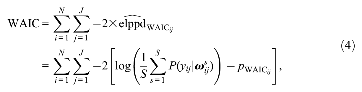
where

The existing literature on the performance of the WAIC in selecting the correct IRT model is limited to unidimensional situations. Thus, it is unclear how this index behaves when used to select among multidimensional IRT models. However, within a unidimensional IRT setting, the WAIC was able to accurately differentiate among the one-, two-, and three-parameter logistic IRT models (Luo & Al-Harbi, 2017) and between unidimensional versions of the GRM and the generalized partial credit model (da Silva et al., 2019). However, to date, no studies have examined how accurately the WAIC can differentiate between non-nested- and nested-dimensionality IRT models.
Log-Predicted Marginal Likelihood
As previously noted, the LPML is an approximation to the LOO based on raw importance sampling. We refer to this index as the LPML rather than the raw importance sampling version of the LOO to differentiate it from the next version of the LOO that we describe shortly. The LPML is based on raw importance ratios, or formally,

leading to
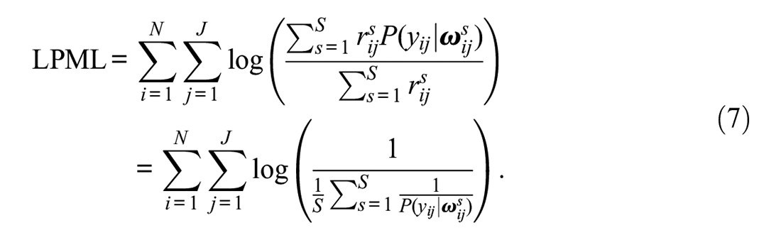
This index is simple to compute, but it could be unstable because the importance ratios could have a high or infinite variance (Vehtari et al., 2017). Nevertheless, the performance of the LPML has been investigated in multidimensional situations. In simulation studies in which nested-dimensionality IRT models (e.g., a bifactor IRT model) and constrained (or more parsimonious) variations of those nested-dimensionality models (e.g., a testlet IRT model) were being compared, with these studies having conditions in which each type of model was the true model, the LPML consistently identified the correct model (Fujimoto, 2018, 2019, 2020; Li et al., 2006). In other words, in these studies, the LPML did not consistently favor the more complex models—potentially making this index less biased toward nested-dimensionality models than the DIC.
In another study, however, the LPML displayed a slight tendency to favor the more complex model when the true model was the bifactor IRT model and the comparison model was a two-tier IRT model, within which the bifactor model is nested—the two-tier model was favored over the bifactor model up to 24% of the time depending on the sample size (Fujimoto & Neugebauer, 2020). These two models, though, were nested-dimensionality models, and the researchers noted that even though the two-tier model was incorrectly favored over the bifactor model in these instances, the estimates from the two-tier model indicated that the model was reduced to a bifactor model, thereby leading to the same substantive conclusion about the dimensional structure of the data as that based on a bifactor model. As of now, it is unclear as to whether the LPML can correctly identify the more parsimonious model in situations in which a unidimensional model is being compared with a bifactor model.
Pareto-Smoothed Importance Sampling–Leave-One-Out Cross-Validation
Vehtari et al. (2022) replaced the raw importance ratios with weights
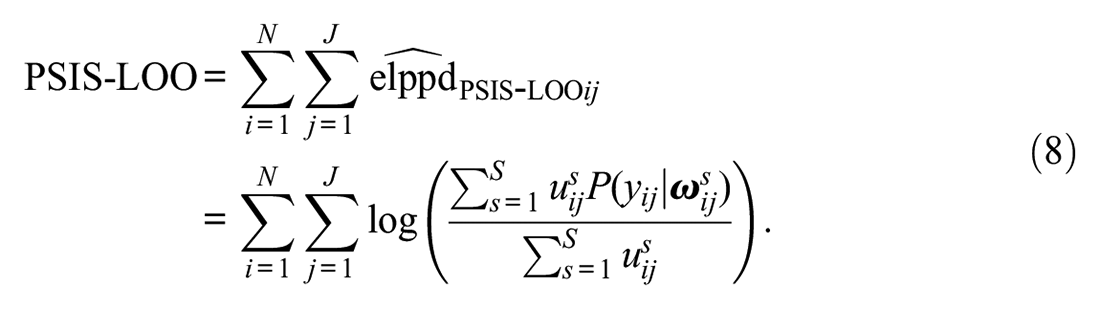
The weights are based on the raw importance ratios in Equation 6, but a smoothing procedure involving the generalized Pareto distribution is applied to the
Similar to the WAIC, the studies that focused on the performance of the PSIS-LOO within IRT are limited to unidimensional settings, and the studies are the same as those we reviewed for the WAIC (da Silva et al., 2019; Luo & Al-Harbi, 2017). In unidimensional situations, overall, the PSIS-LOO identified the correct model, but again, these studies involved differentiating among unidimensional models (e.g., the one-, two-, and three-parameter logistic IRT models). Thus, how capable the PSIS-LOO is at differentiating between non-nested- and nested-dimensionality IRT models has not been investigated.
These Bayesian predictive performance indices have not been studied together to determine whether they can differentiate between nested- and non-nested-dimensionality IRT models, especially when the data represent non-nested-dimensionality structures. In other words, whether the greater fit propensity of nested-dimensionality models leads one or more of these indices to be biased toward those models has not been explored, a void our study fills.
Simulation Study
We conducted a simulation study with a
As for the other variable aspect of the study, the dimensional structures included two non-nested-dimensionality and two nested-dimensionality structures (see Figure 1 for visualizations of these structures). The non-nested-dimensionality structures were a unidimensional and a two-dimensional structure (Figure 1A and 1B, respectively). For the latter structure, the dimensions were correlated at .50, and each item discriminated on only one dimension (i.e., a simple structure), with the items evenly distributed across the dimensions for 15 items per dimension.
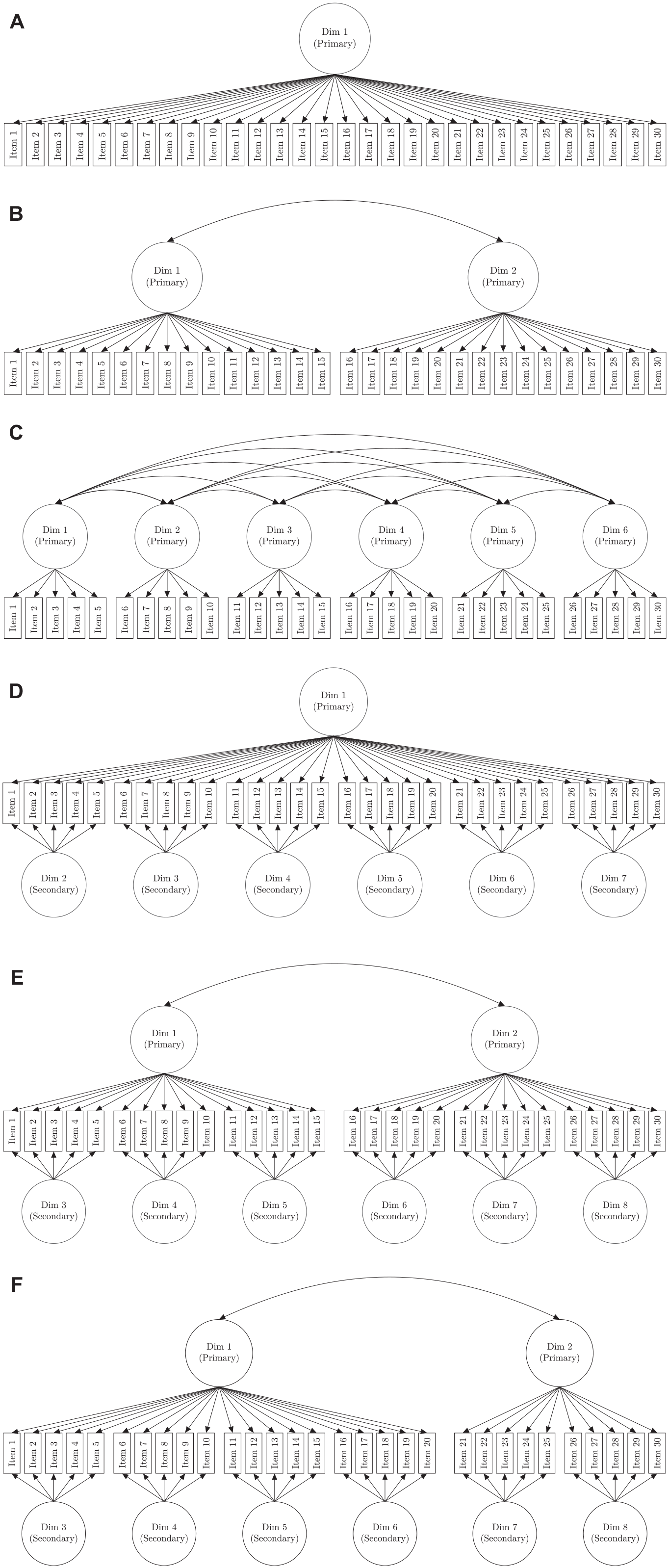
The Following Are Visualizations of the Dimensional Structures to Which the Data Were Generated to Represent (Figures 1A, 1B, 1D, and 1E for the Unidimensional, Two-Dimensional, Bifactor, and Two-Tier Conditions, Respectively) and of the Dimensional Structures Specified for the Models. (A) Unidimensional Structure (Model 1), (B) Two-Dimensional Structure (Model 2), (C) Six-Dimensional Structure (Model 3), (D) Bifactor Structure (Model 4), (E) Two-Tier Structure (Model 5), (F) Alternative Two-Tier Structure (Model 6).
The nested-dimensionality structures were a bifactor and a two-tier structure (Figure 1D and 1E, respectively). The bifactor structure included one primary (or general) dimension and six secondary (or specific) dimensions, with all dimensions being orthogonal to each other. Each item discriminated on the primary dimension and one secondary dimension, with the items evenly distributed across the secondary dimensions. The two-tier structure consisted of two primary dimensions correlated at .50 and six secondary dimensions orthogonal to each other and the primary dimensions. Each item discriminated on one primary and one secondary dimension, with 15 items per primary dimension and five items per secondary dimension.
Analytic Strategy
Models Used
We used six models to analyze each data set. The models included a unidimensional (Model 1), two-dimensional (Model 2), six-dimensional (Model 3), bifactor (Model 4), and two variations of the two-tier IRT model (Models 5 and 6). Models 5 and 6 differed in that Model 5’s dimensional structure matched that of the two-tier condition, and Model 6’s structure was identical to Model 5’s structure in all ways except the first 20 items discriminated on one of the primary dimensions and the last 10 items discriminated on the other primary dimension (rather than 15 items discriminating on each primary dimension, as with Model 5). Visualizations of the dimensional structures specified for the models are also in Figure 1. These models were selected because many of them differed noticeably in complexity but could be competing models, such as the two-tier model having six more dimensions and 30 more item discriminations than the between-item two-dimensional model, or were similar in complexity but had slightly different structures, such as both two-tier models (Models 5 and 6).
These models, then, together with the dimensional conditions, allowed us to determine whether one or more of the predictive performance indices were biased toward nested-dimensionality models and to provide insight into some of the factors that could contribute to the bias. The unidimensional and two-dimensional data generation conditions were where such bias could be revealed. If a predictive performance index is biased toward nested-dimensionality models because of their greater fit propensity, it should favor those models in all dimensional conditions, including the unidimensional and two-dimensional data generation conditions. If the index is not influenced by a model’s fit propensity, then it should favor the nested-dimensionality models corresponding to the data generation models in only the bifactor and the two-tier conditions, and the index should favor the corresponding non-nested-dimensionality models in the unidimensional and two-dimensional conditions. The six-dimensional model (Model 3) was included to be an additional competing non-nested-dimensionality model that was more complex than the unidimensional and two-dimensional models but less complex than the nested-dimensionality models. In addition, the six-dimensional model was included because the nested-dimensionality conditions had six secondary dimensions, and often in model comparisons, nested-dimensionality models are compared with non-nested-dimensionality models that represent the secondary dimensions of the nested structure, with the dimensions allowed to be correlated (e.g., Canivez, 2016).
Technical Details of the Models
All of the models we used were special cases of the multidimensional version of the generalized partial credit model (Muraki, 1992), where the conditional probability of a response of

with the constraint

In Equation 9,
We assigned prior distributions to the parameters that have been shown to lead to models suitable for data representing sample sizes of at least 100 (Fujimoto & Neugebauer, 2020). For these distributions, we use
The latent trait dimensional positions were assumed to be distributed as

where
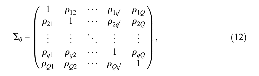
making it a correlation matrix as well. The unique correlations were assigned the prior of

with
Regarding the item parameters, the item discriminations were assigned a prior distribution of

with the mean of the lognormal distribution assigned a hyperprior of

The overall intercepts were assigned a prior of

with

Finally, the relative category intercepts were assigned a prior of

where
The models used in this study were obtained by modifying the sizes of
The MCMC algorithm used to estimate the posterior distributions for all models was written in C++. The algorithm was run for 120,000 iterations for the six-dimensional, bifactor, and two-tier models; the first 20,000 samples were discarded and thereafter every
Model Comparisons
In each dimensional condition, we report the percentage of times each model was favored over all other models. We used the following criteria to determine when a model was favored over another. These criteria addressed model selection uncertainty (Preacher & Merkle, 2012) and identified differences in predictive performances that were more than just trivial. When using the DIC to compare two models (say Model A to Model B), we favored Model A regardless of whether it was the parsimonious model (i.e., the model with fewer estimated parameters) when the difference between their indices, or
When using the LPML, we calculated the pseudo Bayes factor (PsBF) on the two times the log scale, that is,
When using the PSIS-LOO to compare Models A and B, a standard error (SE) of the difference in the PSIS-LOOs can be calculated. Thus, to determine which model was favored, we divided the difference by its corresponding SE, that is,

where

with
For the WAIC, the corresponding
The criteria could make it so that one model is not outright favored over all other models for a data replicate, regardless of the index used. This could occur when both two-tier IRT models (Models 5 and 6) outperform the other models but are equivalent to each other. Because both of these models have similar complexity and the same number of parameters, neither model would be favored, leading to no one model being favored over all other models for that data replicate.
Data Generation
For the unidimensional condition, the latent trait dimensional positions were randomly drawn from
Regarding the item parameters, the nonzero item discriminations were randomly drawn from a uniform distribution ranging from 1 to 3, or
To obtain the data generation values for the items’ overall
Results
The model comparison results are summarized in Tables 1 to 4. In each table, the values in the predictive performance index columns are the averages across the 100 data replicates. Each value in the “%” column indicates the percentage of times the corresponding model was favored over all other models.
Model Comparison Results From the Unidimensional Condition.

Note. The two-tier IRT model with the alternative specification (Model 6) was the version in which 20 and 10 items discriminated on the primary dimensions. Within a predictive performance index section, each value in the “%” column indicates the percentage of times (across the 100 data replicates) the corresponding model was favored over all other models. For example, when using the PSIS-LOO to compare models, the unidimensional IRT model (Model 1) was favored over all other models 100% of the time, whereas none of the other models were favored at any time. DIC = deviance information criterion; LPML = log-predicted marginal likelihood; WAIC = Watanabe-Akaike information criterion; PSIS-LOO = leave-one-out cross-validation approximation based on Pareto-smoothed importance sampling.
The unidimensional IRT model (Model 1) was the data generation model.
Model Comparison Results From the Two-Dimensional Condition.

Note. The two-tier IRT model with the alternative specification (Model 6) was the version in which 20 and 10 items discriminated on the primary dimensions. Within a predictive performance index section, each value in the “%” column indicates the percentage of times (across the 100 data replicates) the corresponding model was favored over all other models. For example, when using the PSIS-LOO to compare models, the two-dimensional IRT model (Model 2) was favored over all other models 100% of the time, whereas none of the other models were favored at any time. DIC = deviance information criterion; LPML = log-predicted marginal likelihood; WAIC = Watanabe-Akaike information criterion; PSIS-LOO = leave-one-out cross-validation approximation based on Pareto-smoothed importance sampling.
The two-dimensional IRT model (Model 2) was the data generation model.
Model Comparison Results From the Bifactor Condition.
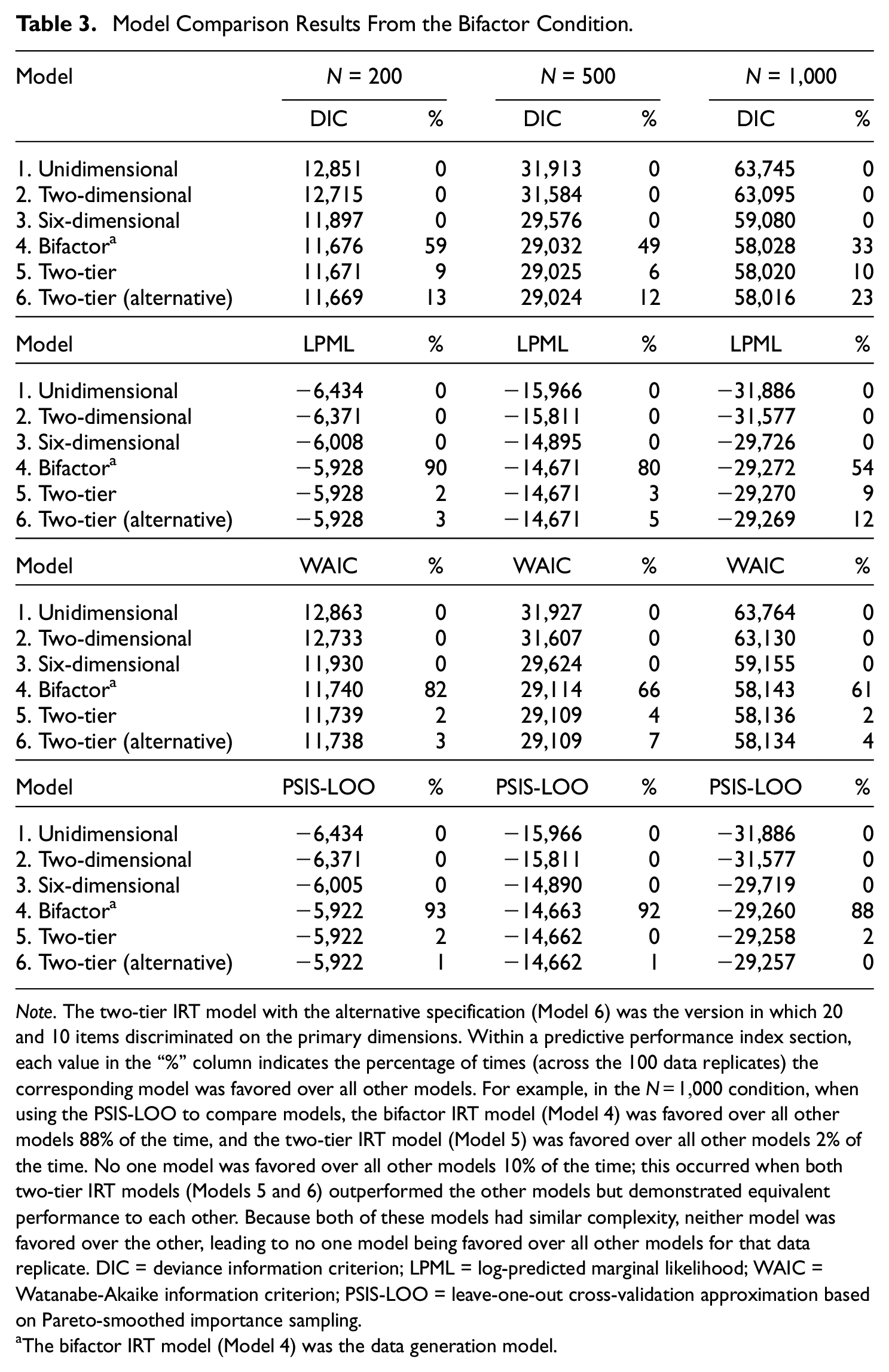
Note. The two-tier IRT model with the alternative specification (Model 6) was the version in which 20 and 10 items discriminated on the primary dimensions. Within a predictive performance index section, each value in the “%” column indicates the percentage of times (across the 100 data replicates) the corresponding model was favored over all other models. For example, in the
The bifactor IRT model (Model 4) was the data generation model.
Model Comparison Results From the Two-Tier Condition.

Note. The two-tier IRT model with the alternative specification (Model 6) was the version in which 20 and 10 items discriminated on the primary dimensions. Within a predictive performance index section, each value in the “%” column indicates the percentage of times (across the 100 data replicates) the corresponding model was favored over all other models. For example, when using the PSIS-LOO to compare models, the two-tier IRT model (Model 5) was favored over all other models at least 99% of the time across all sample size conditions, whereas none of the other models were favored at any time. DIC = deviance information criterion; LPML = log-predicted marginal likelihood; WAIC = Watanabe-Akaike information criterion; PSIS-LOO = leave-one-out cross-validation approximation based on Pareto-smoothed importance sampling.
The two-tier IRT model (Model 5) was the data generation model.
The Unidimensional Condition
The model comparison results from the unidimensional condition are in Table 1. Overall, the LPML, PSIS-LOO, and WAIC outperformed the DIC. Across the sample sizes, the PSIS-LOO favored the data generation model 100% of the time, and the WAIC and LPML favored the correct model at least 96% of the time.
In contrast, when using the DIC, the unidimensional model was never favored over all other models. Instead, the DIC outright favored the bifactor model at least 99% of the time for the sample sizes of 200 and 500. For the sample size of 1,000, the DIC was still biased toward nested-dimensionality models, although it favored the bifactor model less frequently than it did in the other sample size conditions (i.e., 88% of the time) but at the expense of favoring one of the two-tier models more often (i.e., 11% of the time). The nested-dimensionality models being favored would suggest that the data reflected secondary dimensions to be nested within at least one primary dimension. The two-tier models being favored over Model 1 in some instances were not surprising because of the relationship between the two-tier and the bifactor models. As noted earlier, a bifactor model could be viewed as a two-tier model with the correlations among the primary dimensions (i.e., the dimensions in the first tier of the two-tier structure) fixed to 1. Thus, even though the primary dimensional portion of the nested-dimensionality structure consisted of two dimensions for the two-tier models, the correlation between the primary dimensions for each of these models was at least
Although the DIC was biased toward nested-dimensionality models, it fared better when focusing on only the non-nested-dimensionality models and looking at specific pairwise model comparisons rather than the comparisons reported in Table 1, which are across all the models. The DIC correctly favored the unidimensional model (Model 1) over the two-dimensional IRT model (Model 2) at least 97% of the time. However, the DIC’s performance was less consistent across the sample sizes when selecting between Model 1 and the six-dimensional IRT model (Model 3); Model 1 was correctly favored over Model 3 at least 96% and 99% for the sample sizes of 200 and 500, respectively, but only 89% of the time for the sample size of
The Two-Dimensional Condition
The results from the two-dimensional condition are summarized in Table 2. The results show that the LPML, PSIS-LOO, and WAIC outperformed the DIC. However, among the first three indices, the LPML and PSIS-LOO performed slightly better than the WAIC relative to what was observed in the unidimensional condition. In the two-dimensional condition, the data generation model (Model 2) was correctly favored over the other models at least 98% of the time based on the LPML and 100% of the time based on the PSIS-LOO. The WAIC correctly favored Model 2 over the other models at least 90% of the time but no greater than 95% of the time, as observed across the sample sizes.
Regarding the DIC, it again displayed a bias toward nested-dimensionality models. The DIC favored one of the two-tier models over the non-two-tier models 100% of the time, as observed for all sample sizes, with the favored two-tier IRT model (Model 5) being the version in which the primary dimensional structure matched that of the data generation structure. The DIC never favored the bifactor model (Model 4) or the alternative two-tier model (Model 6) in which the primary dimensional portion did not match that of the data generation two-dimensional structure. In fact, when the data generation two-dimensional model (Model 2) was directly compared with the bifactor and the alternative two-tier models, the two-dimensional model was favored 100% of the time, as suggested by the average of the DIC for Model 2 being less than those for the bifactor and the alternative two-tier models within each sample size condition (e.g., for
The DIC also demonstrated some bias toward more complex non-nested-dimensionality models. When focusing on just the unidimensional (Model 1), two-dimensional (Model 2), and six-dimensional (Model 3) models, the DIC correctly favored Model 2 over Model 1 100% of the time. However, the DIC’s ability to correctly favor Model 2 over Model 3 varied depending on the sample size; it favored Model 2 at least 92% of the time when
The Bifactor Condition
The results from the bifactor condition are summarized in Table 3. The four indices never favored one of the non-nested-dimensionality models. However, they varied in how much they favored the data generation bifactor model (Model 4).
Among the indices, the PSIS-LOO was the most accurate, favoring the bifactor model over all other models 88% of the time for
In the instances where the bifactor model was not the most favored, one or both of the two-tier models were favored. It is indicated in Table 3 when only one of the two-tier models was favored over all other models. For example, when
Regardless of whether one or both versions of the two-tier model were favored over the other models, the averages of the posterior means of the correlation between the two primary dimensions (averaged across the 100 data replicates) were at least .96 under Models 5 and 6, suggesting that the two-tier models were nearly reduced to a bifactor model. In this situation, then, the indices incorrectly favoring the two-tier models over the bifactor model are not that misleading because the two-tier models became a bifactor model, thereby leading to the same conclusion about the dimensional structure represented in the data as that based on the true model.
The Two-Tier Condition
The results from the two-tier condition are summarized in Table 4. In this condition, the data were generated to represent a two-tier structure that matched that of Model 5, and all the predictive performance indices favored this model over the other models—including the alternative two-tier IRT model—nearly 100% of the time, if not 100% of the time. The one exception to this was when Model 5 was favored only 93% of the time by the WAIC for
Discussion
Performing model comparisons to evaluate the dimensionality of item response data can be challenging because such comparisons can be biased toward nested-dimensionality IRT models. One reason for the possible bias is that the fit propensity of nested-dimensionality models may be greater than that of non-nested-dimensionality models (e.g., Bonifay & Cai, 2017). However, it is unclear just how much these models’ greater fit propensity can bias model comparison results when working with data representing certain dimensional structures—a situation closer to those seen in practice. The lack of clarity is in part because previous work has not thoroughly evaluated the ability of Bayesian model selection indices to appropriately make adjustments for model complexity and choose the appropriate IRT model from a set of competing models—especially when the set includes non-nested- and nested-dimensionality IRT models.
Our study provides some insight into this issue—that model comparisons being biased could depend on the predictive performance index one uses. We demonstrated that the DIC was severely biased toward nested-dimensionality models (at least within our study conditions). Conversely, the PSIS-LOO was the most accurate at identifying the correct model. It correctly favored the non-nested-dimensionality models in the appropriate conditions 100% of the time. The PSIS-LOO was also mostly accurate at identifying the correct model among a set of nested-dimensionality models; it had a slight tendency to favor the two-tier model in the bifactor condition, although the two-tier model was reduced to a bifactor model, which in turn led to the same conclusion about the dimensional structure being represented in the data as that based on a bifactor model.
Although the PSIS-LOO’s ability to identify the correct model was the greatest among the indices we tested, it was also the most computationally intensive to calculate, which could be a drawback in practice. Thus, the LPML, which was the next best-performing index, could be an alternative to the PSIS-LOO, with the LPML balancing model selection accuracy and ease of calculation. The LPML was nearly perfect at identifying the correct model in every condition except the bifactor condition, where it incorrectly favored the two-tier models more frequently than the PSIS-LOO did. The WAIC’s performance, in general, was similar to the LPML’s. Thus, the WAIC could also be an alternative to the PSIS-LOO, although the LPML is simpler to calculate.
In contrast, the DIC consistently favored the nested-dimensionality models, even when the non-nested-dimensionality models were the true models. In other words, among the indices we examined, the DIC is the most likely to be biased toward nested-dimensionality models. Our findings related to the DIC are consistent with other studies that demonstrated the DIC’s tendency to favor more complex models (e.g., Celeux et al., 2006; da Silva et al., 2019; Li et al., 2006; Plummer, 2008). However, we showed that a certain condition may be required for this tendency to appear in a multidimensional IRT setting—for a nested-dimensionality model to be incorrectly favored over a non-nested-dimensionality model, the dimensional structures the models represent may have to share some features, such as the primary dimensional portion of the structure specified for the nested-dimensionality model may need to match the structure specified for the non-nested-dimensionality model. One example of this was observed in the two-dimensional data generation condition, where only one of the nested-dimensionality models was favored over the data generation model. The favored model was the two-tier model (Model 5) in which the primary dimensional portion of the full dimensional structure matched that of the two-dimensional data generation model. The DIC did not favor the alternative two-tier model (Model 6) or the bifactor model (Model 4) over the two-dimensional model.
Our simulation study, then, demonstrates that the greater fit propensity of nested-dimensionality models does not necessarily lead them to be favored over non-nested-dimensionality models when the latter models are the true models, although which predictive performance index is used matters. Our conclusions, however, should be considered within the context of the study’s limitations. First, we investigated the performance of these indices in four different dimensional contexts, which were selected to determine whether nested-dimensionality IRT models were always favored over non-nested-dimensionality models when the latter models were the true models. There are many types of dimensional structures, but only a limited number can be considered in a single study. Future studies should investigate the accuracy of these indices with other types of nested-dimensionality structures. Second, we fit models that could be applied to all conditions, so we did not fit a simpler bifactor model within which the two-dimensional model was nested (e.g., a version with two secondary dimensions nested within a single primary dimension; Asparouhov & Muthén, 2019). Based on a brief follow-up simulation we conducted, such a model would not add more insight into how these indices are biased toward nested-dimensionality models, given our goal—to determine whether Bayesian predictive performance indices tend to be biased toward nested-dimensionality models. However, future studies should investigate other instances where simpler, nested-dimensionality models are included in more applicable dimensional conditions to understand further how these models’ complexity and their relationship to non-nested-dimensionality models affect the performance of these indices.
The third limitation is that we compared the
Last but not least, we relied on simulated data generated to clearly represent certain dimensional structures. In practice, the data may not clearly reflect one of the dimensional structures represented by the models being compared, such as in Greene et al. (2019). However, if these indices do not perform optimally in ideal situations in which the correct answer is known, then these indices cannot be trusted in less-than-optimal conditions. Thus, we concentrated on establishing how well these indices functioned in ideal situations, with the models being distinctly different for the most part. However, future research should investigate the performance of these indices in less optimal situations.
Even with these limitations, our study challenges the notion of the broader literature that models with greater fit propensity automatically bias model selection results toward those models, although the predictive performance index one uses matters. Given our study conditions, the DIC is most likely to lead to the pitfall of favoring nested-dimensionality models over non-nested-dimensionality models when the latter are more appropriate for the data, thereby misguiding researchers to conclude that more complex dimensional structures are represented in their data. However, such a misstep may be avoidable with the PSIS-LOO.
Supplemental Material
sj-pdf-1-epm-10.1177_00131644231165520 – Supplemental material for The Accuracy of Bayesian Model Fit Indices in Selecting Among Multidimensional Item Response Theory Models
Supplemental material, sj-pdf-1-epm-10.1177_00131644231165520 for The Accuracy of Bayesian Model Fit Indices in Selecting Among Multidimensional Item Response Theory Models by Ken A. Fujimoto and Carl F. Falk in Educational and Psychological Measurement
Footnotes
Declaration of Conflicting Interests
The authors declared no potential conflicts of interest with respect to the research, authorship, and/or publication of this article.
Funding
The authors received no financial support for the research, authorship, and/or publication of this article.

Supplemental Material
Supplemental material for this article is available online.
References
Supplementary Material
Please find the following supplemental material available below.
For Open Access articles published under a Creative Commons License, all supplemental material carries the same license as the article it is associated with.
For non-Open Access articles published, all supplemental material carries a non-exclusive license, and permission requests for re-use of supplemental material or any part of supplemental material shall be sent directly to the copyright owner as specified in the copyright notice associated with the article.
