
Abstract
Increasingly, researchers are focusing on the study of environmental values of young people. Indeed, it is today’s youth who will be the decision makers in the future. Attention has turned to explaining individual differences in this construct, and many authors have illustrated gender differences. The current study (N = 1,285, 10- to 12-year-olds) compares results of a classical analytical approach to quantifying such differences (independent samples t tests) with one of measurement and structural invariance across genders. The essential difference between the two is that whereas the latter controls for differential item functioning across gender, the first does not. The results show that whereas gender differences in utilization values occur when applying a classic analytical approach, they do not occur through the invariance approach. These results suggest that other studies that demonstrated gender differences might be explained by differential item functioning rather than reflect genuine differences, and might thus represent methodological artifacts.
Environmental Values (EVs)
Within the fields of environmental education, psychology, and sociology, EVs have been studied extensively. The term EV attempts to describe how people view the natural environment and their relationship to it. Social psychologists regard this as the endorsement of a fundamental paradigm, and the term mainly taps into what, in social psychology, are called “primitive beliefs” (Stern, Dietz, & Guagnano, 1995) about the nature of the earth and humanity’s relationship with it. These primitive beliefs form the inner center of an individual’s belief system and represent that individual’s basic truths about physical and social reality (Rockeach, 1968).
Within the framework of the two-dimensional model of EVs (2-MEV; Bogner & Wiseman, 2006), the term values stems from a convention established by Rockeach (1968) that indicates a set of closely related attitudes. Thus, first-order factors are labeled attitudes, and higher order factors are labeled values. The first results with regard to the development and application of the 2-MEV were published in the mid-90s (Bogner & Wilhelm, 1996), and through several follow-up studies, the scale was refined (e.g., Bogner & Wiseman, 2002). The item battery used in the scale initially quantified five distinct environmental attitudes via first-order factors (“intent of support,” “care with resources,” “enjoyment of nature,” “altering nature,” and “human dominance”), but the emphasis in the research using the 2-MEV has moved to values via two higher order factors (Bogner & Wiseman, 2006; Oerke & Bogner, 2010). This two-factor model was formalized as follows:
Environmental values are determined by one’s position on two orthogonal dimensions, a biocentric dimensions that reflects conservation and the protection of the environment (Preservation or P); and an anthropocentric dimension that reflects the utilization of natural resources (Utilization or U). (Wiseman & Bogner, 2003, p. 5)
The 2-MEV’s framework allows individuals to be placed in one of four quadrants, rather than on either end of a continuum; the factors’ orthogonality permits a respondent to vary his or her position on one dimension independently of that on the other. The model therefore does not imply a conflict between assigning high importance to the protection of the environment and to the need to make use of natural resources. Milfont and Duckitt (2004) pointed out that this two-dimensional framework is therefore consistent with the contemporary sustainable development (SD) debate: It does not impose a rejection of one’s persuasion when one accepts another, but rather allows for an integrated set of values that can be (but does not have to be) in favor of the preservation and the utilization of natural resources. The two-dimensional framework has been confirmed by several independent scholars in Flanders (Boeve-de Pauw & Van Petegem, 2011a), across 16 European countries (Munoz, Bogner, Clement, & Carvalho, 2009), in several non-European countries (Brazil, New Zealand, and South Africa; Milfont & Duckitt, 2010; Vietnam and Guatemala; Boeve-de Pauw & Van Petegem, 2011a), and in the United States (Johnson & Manoli, 2011).
EVs and Gender
Sociodemographics have received a great deal of attention in the research on EVs and environmental engagement, and typically, gender is seen as a major explicator of individual differences. Gender differences have been illustrated for adults (Schahn & Holzer, 1990), young adults (Goldman, Yavetz, & Pe’er, 2006), and children (Zelezny, Chua, & Aldrich, 2000); for each of these age groups, woman (and girls) have been shown to hold more pro-EVs or pro-environmental engagement than men (and boys). A widely used approach to explain these gender differences is based on gender roles and socialization (Zelezny et al., 2000). Socialization theory posits that individuals are shaped by gender expectations within the context of cultural norms. Females across cultures are socialized to be more expressive, to have a stronger ethic of care, and to be more interdependent, compassionate, nurturing, cooperative, and helpful in caregiving roles; males, however, are socialized to be more independent and competitive (Eagly, 1987). These differences in socialization between the genders could then be reflected in pro-environmental attitudes and behavior (Zelezny et al., 2000).
Researchers who use one-dimensional scales to quantify EVs typically find that woman score “better” (i.e., are more ecocentric) than men (e.g., Blaikie, 1992). However, authors who apply the two-dimensional framework of the 2-MEV have shown more nuanced differences between the genders; Oerke and Bogner (2010), for example, showed that woman hold less utilitarian values than men, whereas no gender differences were found for preservation values. Boeve-de Pauw and Van Petegem (2011b) showed the same pattern in gender differences in the EVs of children. Milfont and Duckitt (2004), however, showed that women displayed higher preservation values than men and found no gender differences for utilization values. The results of these studies illustrate the added value of applying the two-dimensional framework of the 2-MEV when assessing differences between individuals: The two higher order factors (or values) can be affected separately. Applying a one-dimensional framework might blur such effects.
If one is interested in fully grasping differences between groups, then it is important not only to use an instrument that builds on a framework that allows for proper measurement but also to know whether the instrument measures the same psychological construct in the same way in all groups (Milfont & Fischer, 2010)—in other words, whether the measure is equivalent for individuals from different groups. If this is not the case, the observed results might spring from a differential instrument functioning rather than reflect genuine differences. Within psychological measurement practice, this kind of equivalence in the functioning of instruments is known as invariance (Byrne, Shavelson, & Muthén, 1989); establishing invariance is essential to make meaningful comparisons across groups (Rusticus & Hubley, 2006). Several studies have shown that gender role socialization can exist at different levels (e.g., Foels & Reid, 2010; Rusticus & Hubley, 2006); women and men can, for example, differ not only in how they relate to or attribute importance to perceive a certain issue (such as environmental problems) but also in how they conceptualize that issue. Gender differences might be present at the construct level as well as at the level of item interpretation or functioning.
To comprehensively study gender differences in EVs, the present study focuses on gender differences in EVs through two different methodological approaches; on one hand, the genders’ EVs (as tapped by the 2-MEV) are compared using traditional analyses of variance technique, and on the other hand, the invariance of the 2-MEV across gender is assessed.
Testing Invariance
Milfont and Fischer (2010) detailed that psychological constructs such as EVs constitute latent variables that cannot be measured directly. As a result, psychological measures function as indicators of the latent construct. Factor analytical techniques are frequently used to map the relationship between latent variables (or factors) and their indicators (or items).
To meaningfully compare factors across distinct groups (such as countries, gender, majors), or across time, each item must relate to the factor in the same way in each group. Often, establishing reliability and construct validity is regarded as being sufficient to make valid comparisons between groups (Steinmetz, Schmidt, Tina-Booh, Wiezczorek, & Schwartz, 2009). This is, however, often not justified, and the assumption should be evaluated explicitly by testing for invariance (Milfont & Fischer, 2010). Invariance focuses on the equivalence of factors across different groups and centers around two issues: measurement invariance and structural invariance (Byrne et al., 1989). Measurement invariance, on one hand, assesses the invariance of the basic model structure, factor loadings, item intercepts, and error variances, whereas structural invariance, on the other hand, assesses the invariance of factor variances, factor covariances, and factor means.
Whereas the necessity for establishing structural invariance depends on the research questions under consideration, testing for measurement invariance is indispensable when the aim is to compare groups in a meaningful way (Milfont & Fischer, 2010). Violations of measurement invariance assumptions can be equally threatening to substantive interpretations as the inability to demonstrate reliability and validity (Vandenberg & Lance, 2000). If measurement invariance is not tested, interpretations of between-group comparisons are problematic (Vandenberg & Lance, 2000). Absent invariance, observed differences in means or other statistics might reflect differences in systematic biases of response across groups or different understanding of the concepts, rather than substantive differences (Steenkamp & Baumgartner, 1998). Equally important, findings of no difference between groups do not ensure the absence of “real” differences.
Measurement Invariance
The meaning of measurement invariance is “whether or not, under different conditions of observing and studying phenomena, measurement operations yield measures of the same attribute” (Horn & McArdle, 1992, p. 117). Multigroup confirmatory factor analysis (MGCFA; Jöreskog, 1971) is among the most powerful techniques for testing measurement invariance. Steenkamp and Baumgartner (1998) proposed stepwise procedural guidelines for assessing measurement invariance, from the least to the most demanding form of invariance.
The lowest level of invariance is configural invariance. This requires that the items in an instrument display the same configuration in each of the different groups, that is, if the basic model structure is invariant across groups. This form of invariance indicates that respondents from the different groups conceptualize the constructs in the same way. Configural invariance, however, does not ensure that respondents in different groups understand each of the items in the same way. Although the same items form a factor that represents each construct, the factor loadings may be different across groups.
The next level therefore is metric invariance, which requires that factor loadings are invariant across groups. It is tested by restricting the factor loading of each item on its corresponding construct, to ensure that it is the same across groups. Configural invariance and metric invariance are tested by examining only information about covariation among items.
A third level of invariance is necessary to justify comparing the means of the underlying constructs across groups. Such comparisons are only meaningful if the items exhibit scalar invariance. This form of invariance indicates that differences between groups in the means of the observed items result from differences in the means of their corresponding constructs. To assess scalar invariance, the intercepts of the underlying items are constrained to be equal across groups; in the case of ordered-categorical data, the thresholds between the response categories are constrained.
A fourth step in the procedure for testing measurement invariance is that of checking the invariance of error variances. Including this last step in the procedure is often referred to as strict invariance, and is seen as optional, or even as too strict by some authors (Dimitrov, 2006).
If all levels of the procedure are met, full measurement invariance can be presumed. In practice, however, full measurement invariance is unlikely to be met (Hoyle & Smith, 1994), and at least partial measurement invariance should be established. This implies that a subset of parameters in a model is constrained across groups, while another subset is allowed to vary (Milfont & Fischer, 2010). Thus, measurement invariance can be regarded as the degree to which the model’s parameters are invariant (Dimitrov, 2006). Although Byrne et al. (1989) state that at least one of the multiple indicators (or items) other than the one fixed to 1.00 for identification purposes needs to be invariant (Byrne et al., 1989), the question as to what degree partial measurement invariance is acceptable is under debate (Gregorich, 2006). For example, partial invariance of the underlying measurement model may be sufficient when applying a structural equation modeling approach but not when using composite scores or sum scores into which the invariant and noninvariant items are aggregated (Steinmetz et al., 2009). There is no rule of thumb; it is up to the researcher (depending on the specific research question) to decide to what extent measurement invariance can be partial, as long as the degree of invariance is reported with the results (Dimitrov, 2006).
Structural Invariance
Models that concern only the latent variables are structural invariance tests. Three are common in this category: factor variance invariance, factor covariance invariance, and factor mean invariance. Whereas the different models that need to be fitted to establish measurement invariance need to be hierarchically nested, the different models for structural invariance do not; each of the conditions for structural invariance can be tested separately after measurement invariance has been established. As argued above, testing for measurement invariance is required when the focus is on comparing groups; testing structural invariance is only needed when a specific (structural) research question needs to be answered (Milfont & Fischer, 2010).
Invariance of factor variance indicates that the range of scores on a factor does not vary across groups. Constraining all factor variances across groups can test this condition. Invariance of factor covariance implies that all factors have the same relationship in all groups. Constraining all factor covariances across groups can test this condition. Invariance of factor means indicates that groups score the same on the factor. Again, constraining all factor means across groups can test this condition.
The Present Study
In the present study, the results of two approaches to studying gender differences in EVs are presented. The first is through a classical t test, and focuses on differences in mean scores. Three scenarios are included in this first approach, differing in the way sum scores were calculated: (a) as the average across all 2-MEV items (10 for Preservation and 10 for Utilization), (b) as the average across those items that result from an exploratory factor analysis (EFA; performed on the data in this study), and (c) as the average of the same items in Scenario 2, but corrected for their factor loading. The second approach applies invariance testing across gender and (after having tested for configural, metric, and scalar invariance) addresses the topic as an issue of structural invariance.
The central issue of this study is then whether gender differences in the EVs of children are genuine or whether they might be due to the methods applied. In other words, do different methodological approaches of quantifying gender differences in EVs come to different results?
Method
Respondents
In total, 1,285 children from 59 Flemish schools participated in the study; all were in the last year of primary education. The respondents’ ages ranged from 10 to 12 years, with a mean age of 11.23 ± 0.55. The gender ratio (boys:girls) was 0.96 with 626 boys and 652 girls (and 9 unknown). In total, 90 schools were invited to participate in the study. The response rate at the school level was 66%. Within each school, a single class was asked to participate: Respondents were therefore clustered in a two-level hierarchy, namely, children within schools. The mean class size was 19.75 ± 7.61 children. Before administering the questionnaire, a pilot was run for item comprehensibility, difficulty, and interpretation, with a small group of 30 children who were not included in the final sample. No notable problems were reported.
The Two-Dimensional Model of Ecological Values
The respondents’ EVs were tapped using Bogner and Wiseman’s (2006) two-dimensional model of ecological values. In earlier versions of the scale, 69 items were used from other attitudinal scales to measure “environmental concern” (Bogner & Wilhelm, 1996). The results revealed several subscales of environmental concern, including distinct attitudes. In further work (e.g., Wiseman & Bogner, 2003), the main focus moved away from the first-order factors (attitudes) and toward second-order factors (values). In 2006, Bogner and Wiseman published the results of a study that quantified the 2-MEV model; out of the pool of all previously used items, 20 were distilled to tap EVs. They thus presented the 2-MEV as an instrument with two subscales, each one designed specifically to tap one of the two second-order factors (or values): Preservation and Utilization. Both factors are measured by 10 items on a 5-point Likert-type scale (ranging from strongly disagree to strongly agree, with a neutral agree nor disagree in the middle). A sample item for the preservation factor of environmental attitudes is, “We must set aside areas to protect endangered species.” A sample item for the utilization factor of environmental attitudes is, “We need to clear forests in order to grow crops.” All 20 items (as shown in Table 1) were administered to the respondents.
The 20 Items of the 2-MEV and Their Factor Loading Resulting From the EFA.

Note: 2-MEV = two-dimensional model of environmental values (Bogner & Wiseman, 2006); EFA = exploratory factor analysis. Absent factor loadings indicate items that loaded below .3 in the EFA.
Analyses
The normality of each item was tested and found to be within the level recommended for (CFA; skewness < 2, kurtosis < 7; West, Finch, & Curran, 1995). We also tested for multivariate outliers; one respondent was a multivariate outlier at the item level (with a maximum Mahalanobis distance to the centroid of 55.49, which is above the critical value of 45.31) and one at the construct level (with a maximum Mahalanobis distance to the centroid of 18.73, which is above the critical value of 16.27). Because we only had a few outliers (two in a total sample of 1,285), and their scores did not greatly exceed the critical value, we left the respondents in the data, as recommended by Tabachnick and Fidell (2007).
As a previous study (Boeve-de Pauw & Van Petegem, 2011b) showed that the Flemish version of the 2-MEV differed from the original 2-MEV by Bogner and Wiseman (2006), the first step in the present was to examine the factor structure by means of an EFA. For this EFA, a random part (n1 = 429) of the data set was used, while the remaining data (n2 = 850, n2,boys = 416, n2,girls = 434, and a drop-out of six due to unknown gender) were used for the t tests, the CFA, and the MGCFA (see below). The EFAs were performed using the weighted least squares mean (WLSM) estimator and an oblique geomin rotation (the default in Mplus when performing an EFA with categorical data). The number of factors was selected based on the eigenvalues greater than one rule (Bandalos & Boehm-Kaufman, 2009), the observed drop in eigenvalues (Tabachnick & Fidell, 2007), and the interpretability of the factors. Only factors including more than two items and items with loadings greater than |.3| on only one factor were retained (Tabachnick & Fidell, 2007).
In a second step, t tests were performed to compare the genders’ EVs following three distinctly different scenarios. In the first scenario, all twenty 2-MEV items (10 for Preservation and 10 for Utilization) were included, and scale scores were calculated as the average across the items. In the second scenario, only those items that resulted from the EFA were retained; scale scores were calculated as the average across the retained items. In the last scenario, the same items resulting from the EFA were used, but scale scores were corrected for their factor loading (thus acknowledging that the different items have a different weight in the latent constructs). For each scenario, the genders’ EVs were then compared using a classical independent samples t test. All t tests were performed in SPSS 18.0.
When multiple tests are run on the same data, it is common practice to adjust the α-level (p = .05) to the number of tests run, not to inflate the chance of obtaining statistically significant results. Such practices have, however, been shown to have no principled basis (Perenger, 1998) and even to be deleterious to sound statistical inference (O’Keefe, 2003). We did therefore not adjust the α-level to the number of tests.
In the third step, configural invariance was tested for the factor structure that resulted from the EFA. Two separate CFAs for each gender group were conducted. To evaluate model fit, multiple fit indices were used, with a minimum value around .95 for the comparative fit index (CFI) and the Tucker–Lewis index (TLI), and a value of .06 or less for the root mean square error of approximation (RMSEA; Tabachnick & Fidell, 2007). Where necessary, modification indices (MIs) were used to identify how to improve model fit. Items with high MIs toward other factors than those that they were intended to tap were deleted because these items might tap into multiple constructs. Furthermore, the MIs were also used to add error covariances between items of a same factor, to further obtain a more realistic and better fitting model (Byrne, 1993). Items were always deleted, and error covariances were always added for both gender groups, unless MIs were nonsignificant for both groups.
The fourth step was to test for the other levels of measurement invariance—metric and scalar invariance—by means of MGCFA. Because the data are ordered-categorical data, the weighted least squares mean and variance (WLSMV) estimator with delta parameterization was used. A series of nested models were tested, following the recommendations of Muthén and Muthén (1998-2007) when testing measurement invariance with categorical data. In the first, unconstrained model, the factor loadings and thresholds were allowed to differ across groups, with the scale factors fixed at one and factor means fixed at zero in all groups. This allowed us to establish a baseline model that could be used to further test consecutive, more restrictive models by means of the chi-square difference test. In the second model, factor loadings and thresholds were constrained to be equal with the scale factors fixed at one, and the factor means fixed at zero in one group and free in the other. The factor loadings and thresholds were not constrained separately with first testing for metric invariance and subsequently for scalar invariance. Instead, factor loadings and thresholds were constrained simultaneously, because for categorical outcomes, the item probability curve is influenced by both parameters (Muthén & Muthén, 1998-2007).
To test for measurement invariance of the factor loadings and thresholds, the chi-square difference test was used, also taking the differences in fit indices into consideration (Vandenberg & Lance, 2000). For these fit indices, a change of −0.01 or more in CFI or TLI, and a change of 0.015 or more in RMSEA, indicates noninvariance (Chen, 2007). For the chi-square difference test, a nonsignificant difference between the chi-square value of the more and less restrictive models supports measurement invariance, whereas a significant difference in chi-square does not. With categorical data using the WLSMV estimator, the conventional approach of just taking the difference in chi-square values and degrees of freedom between models is not appropriate because this difference in chi-square has no chi-square distribution (Muthén & Muthén, 1998-2007). Therefore the chi-square difference test function in Mplus was used, which runs a correction of the chi-square value. When the difference using this test was significant (p < .05), only partial measurement invariance could be established.
To determine the degree of partial measurement invariance, the model was modified by freeing parameters. The order of setting parameters free was determined by the value of the MI (which gives the expected drop in the model chi-square value when this parameter is estimated freely). MIs are significant when they exceed 3.84 (Dimitrov, 2006). First, the parameters for the item with the largest significant MI were set free. Given that our data are categorical, equality constraints for the thresholds and factor loadings were relaxed simultaneously. After freeing the factor loadings and thresholds of the first item, the model was refitted. When the chi-square difference test was still significant, other parameters were relaxed. When there was no difference in the chi-square (partial) measurement, invariance was achieved (Dimitrov, 2006).
The fifth and final step was to test for the structural invariance of gender means. The model that resulted from the MGCFA was further used to test for invariance of factor means. Parameters that had been relaxed due to noninvariance in previous steps were also relaxed between groups when testing for factor mean invariance. Factors means were constrained to be equal by fixing them at zero in both groups (Muthén & Muthén, 1998-2007), and the DIFFTEST function was used to check for structural invariance. Invariance of the factor means is not supported when the models differ significantly. In this case, MIs show for which factor(s) the equality constraint for the mean across groups needs to be relaxed. Relaxing factor means according to the MIs is analogous to relaxing parameters when testing partial measurement invariance as described above. First, the factor mean with the highest MI is relaxed, and the model is then tested again. If the chi-square difference is still significant, other means are relaxed until the chi-square difference test is not significant, and the mean invariance testing can be finalized.
All factor analyses were conducted using the Mplus software (Muthén & Muthén, 1998-2007). The fact that we were dealing with ordered-categorical data (by using the WLSM or WLSMV estimators) and the nonindependence of respondents (by using the type=complex function) were accounted for.
Results
EFA
An EFA yielded five factors with an eigenvalue above 1; a drop in eigenvalues was observed after the second factor. This five-factor solution did not provide a meaningful interpretation; several items had to be deleted due to cross-loadings, and most of the factors were left with just two or three items. To be able to accept the four-factor solution, four items would have had to be omitted due to cross-loadings and two items due to loadings below |.3|, which would have left two interpretable factors. A two-factor solution was run, and Items U2, U7, and U9 had to be omitted due to cross-loadings and Item U1 due to loading below |.3|. Furthermore, Item P4 was excluded because it loaded on Factor 2 while being designed to load on Factor 1, suggesting that the respondents misinterpreted the item. In conclusion, the EFA yielded a two-factor structure with nine items loading on the first factor and five items loading on the second. These two factors, respectively, correspond to Bogner and Wiseman’s (2006) Preservation and Utilization. Table 1 reports the factor loading for those items that showed values above |.3| in the EFA.
t Tests for Independent Samples
The first scenario within this analytical phase was to compare the genders’ EVs using all twenty 2-MEV items (10 for Preservation and 10 for Utilization). Scale scores were—for each dimension—calculated as the average of the 10 included items. As Table 2 illustrates, an independent sample t test revealed that boys and girls did not differ on the preservation dimension, but that boys do show a higher mean value than girls on the utilization dimension. In the second scenario, scale scores were calculated as the average of the scores for the items that resulted from the EFA reported above. Again no differences were observed for the preservation dimension, and again boys showed a higher mean value than girls for the utilization dimension. In the third scenario, scale scores were calculated as the standardized sum of the scores for each item corrected for its factor loading in the EFA. The scale scores were standardized because while correcting the items for their factor loading acknowledges that different items have different weights in the latent constructs, it also renders the scores incomparable across the two dimensions and across the different t tests that were performed. Again no differences were observed for the preservation dimension, and again boys showed a higher mean value than girls for the utilization dimension. Table 2 presents an overview of the three scenarios.
Results From the Three Different Scenarios Within Which Independent Samples t Test Were Performed.
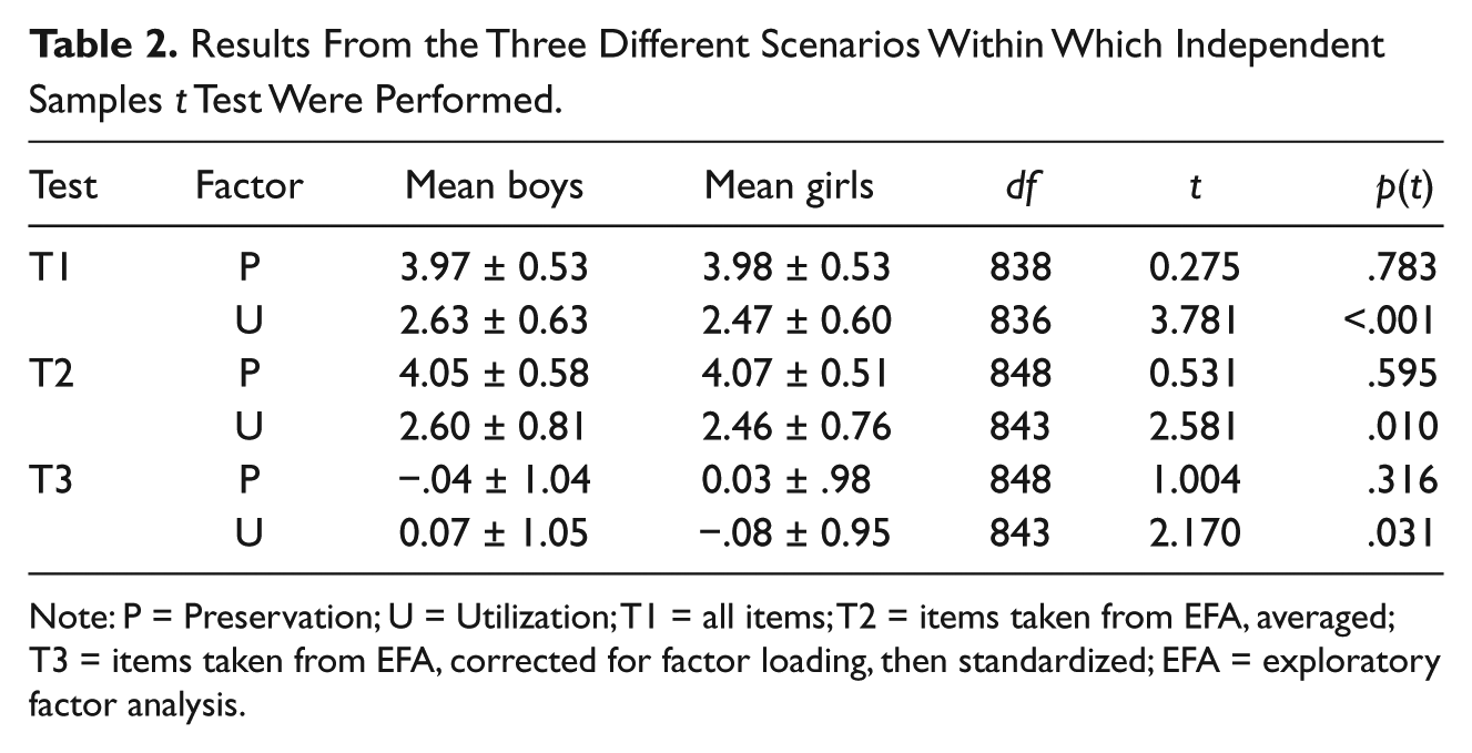
Note: P = Preservation; U = Utilization; T1 = all items; T2 = items taken from EFA, averaged; T3 = items taken from EFA, corrected for factor loading, then standardized; EFA = exploratory factor analysis.
Configural Invariance
The model that resulted from the EFA was tested in two separate CFAs for configural invariance across the genders. Fit indices for both CFAs are presented in Table 3 and indicate that the model did not fit to the data for either boys or girls. The MIs indicated that Item P9 had a high link with Factor 2, and more specifically with Item U4, suggesting that Item P9 measures both constructs. The item was omitted from further analyses. Refitting the model without Item P9 still yielded fit indices below the level of acceptance. The MIs suggested that incorporating error covariances would enhance model fit. Including covariance between Items P2 and P5, and between P6 and P7, resulted in a good model fit for the boys. For the girls, however, an additional error covariance between Items U3 and U4 was included to achieve model fit. Although adding this third error covariance for boys also resulted in a good fitting model, we decided not to include it because the items were not correlated significantly for the boys. The model without Item P9 and with two and three error covariances, respectively, for boys and girls was used as the basis for further tests for metric and scalar invariance.
Fit Indices for the Confirmatory Factor Analyses.
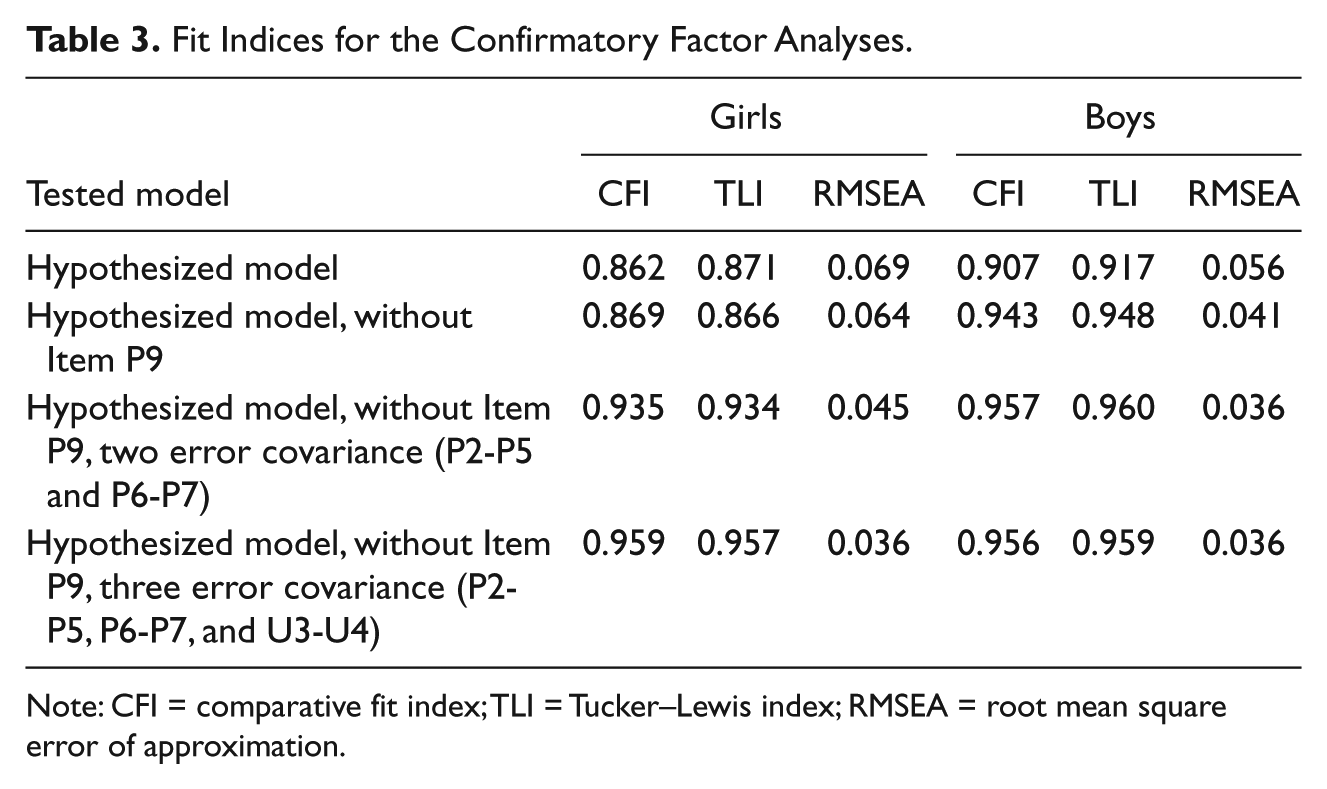
Note: CFI = comparative fit index; TLI = Tucker–Lewis index; RMSEA = root mean square error of approximation.
The covariance between Items P2 and P5 reflects the attitude enjoyment of nature; the one between Items P6 and P7 reflects care with resources. The error covariance between U3 and U4 reflects altering nature. The fact that these first-order factors are (to some extent) still present in the instrument is, in essence, not problematic, as long as they are accounted for by including error covariances, which results in a more realistic and better fitting model (Byrne, 1993).
Metric and Scalar Invariance
Invariance of the factor loadings and thresholds across the genders was tested with a MGCFA. Fit indices for the consecutively estimated models are presented in Table 4. A measurement noninvariance model without constraints on any of the parameters was tested first and used as a baseline or comparison model for the subsequent models. The results indicate that full measurement invariance cannot be accepted: When comparing this baseline model with the full measurement invariance model, the chi-square difference test was significant, and the changes in CFI and TLI were above 0.01. To establish partial measurement invariance, parameters were relaxed step by step, based on the MIs. First, Item U3 was relaxed across the genders because it showed the highest MI, but the fit indices did not indicate that partial measurement was established. Therefore, the loading and thresholds of Item P3 and subsequently of Item P8 were also relaxed. This led to a good fitting model and a change smaller than 0.01 and 0.015 in the TLI and RMSEA, respectively. However, with a p value below .05, the chi-square difference test indicated that the model with three relaxed items still significantly differed from the baseline model. The parameters of one additional item (U5) were relaxed.
Fit Indices for the Multigroup Confirmatory Factor Analyses.
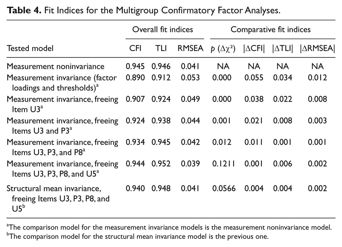
The comparison model for the measurement invariance models is the measurement noninvariance model.
The comparison model for the structural mean invariance model is the previous one.
Table 5 gives an overview of the factor loading of the four items that were noninvariant. The factor loadings in this table were derived from the measurement invariance model. For Item P3, the fourth threshold was not significant for the boys, whereas for the girls it was. The same goes for the first threshold of Item U3. For each of these items, MI indices for relaxing the loading and threshold indicated that the model would improve significantly. It should be noted that the information in Table 4 needs to be interpreted with care because loadings and thresholds are interdependent when dealing with ordered-categorical data, and were therefore relaxed simultaneously in the consecutively estimated models. With the factor loadings and thresholds of these four items relaxed across groups, partial measurement invariance was established.
Factor Loadings for the Four Noninvariant Items, As Derived From the Partial Measurement Invariance Model
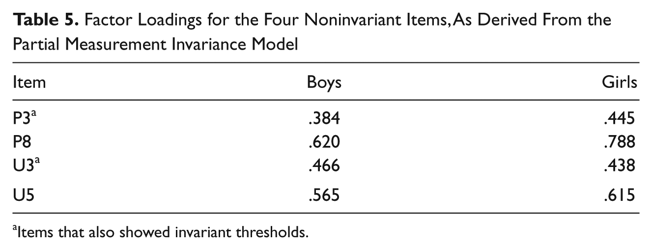
Items that also showed invariant thresholds.
Structural Invariance
Subsequently, this partial measurement invariant model was used to test the structural invariance across the genders. The results in Table 4 show that there is no significant difference in chi-square between the model with constrained factor means and the previous model with four noninvariant items. As the p value of the chi-square difference test was .056 (and thus neared significance), despite the small but significant MIs, we also checked the invariance of both factor means separately. This yielded p values for the chi-square difference test of .143 and .608, respectively, for the model with the first factor mean constrained and for the second factor mean constrained. These results confirm that the factor means are invariant across groups: Consequently, the hypothesis of equal means for boys and girls cannot be rejected.
The correlation between the two latent factors Preservation and Utilization was also included in the MGCFA at this stage, and was estimated at −.107 for the boys and −.119 for the girls. A model imposing the invariance of these estimates across the genders did not differ significantly from the comparison model, suggesting that the correlation does not differ across the genders.
Discussion
The aim of the present study was to examine whether gender differences in EVs are genuine findings or whether they might reflect methodological artifacts. We therefore focused on gender differences through two different methodological approaches: (a) classical independent samples t tests and (b) a measurement invariance analysis.
The Three t Test Scenarios
Gender differences were estimated through several independent samples t tests. Three different scenarios were followed, each representing a technique of calculating scale scores that is common in the social sciences. In the first scenario, all items were used regardless of whether factor analytical techniques attributed them to a given factor. In the second, based on an EFA, only items belonging to the factor were included. The final scenario then corrected those items for their factor loading.
Although the results of the different t tests show that no differences occurred for preservation values, boys did display higher utilization values than girls in each of the three scenarios. These findings are consistent with those of authors such as Oerke and Bogner (2010) and Boeve-de Pauw and Van Petegem (2011b). Although with each next scenario included in this analytical step, the calculation of the scale scores and the scale means includes less error, this approach assumes that the items that underlie the psychological constructs of preservation and utilization function equivalently for boys and girls. Possible differences in item functioning between boys and girls are not accounted for in this approach; this is the essential difference with the second approach, that of measurement invariance.
Measurement Invariance
The results of the MGCFA showed that full measurement invariance could not be established because the factor loadings of four items (P3, P8, U3, and U5) were noninvariant across the genders. It is difficult to explain why these items function differently for boys and for girls. Possible answers might be found in the use of words across items that appeal more to one gender than to the other, and which might result in a differential item functioning. Alternatively, the differences might be due to differences in the response style of boys and girls. Girls might, for example, be inclined to answer more negative when it comes to items concerning the utilization of the environment and natural resources than boys. Such response style differences have been demonstrated between the genders in, for example, the prevalence of depression (Van de Velde, Bracke, Levecque, & Meuleman, 2010), coping strategies (Piko, 2001), self-esteem (Bachman, O’Malley, Freedman-Doan, Trzesniewski, & Donnellan, 2011), and so on.
Different response styles may be due to socialization processes that contribute to gender stereotypes. Eagly (1987) describes such gender stereotypes as females having a stronger ethic of care, and being helpful and caregivers; males, however, are socialized to be more independent and competitive. Zelezny et al. (2000) suggest that socialization is the most widely used approach to explain gender differences in environmentalism. It could be so that socialization does indeed explain such differences but that it does so through impacting the response style of girls and boys differently rather than shaping their EVs. Whichever explanation is at the root of the differences observed in the means, the current study illustrates that for EV (as tapped with the 2-MEV), they disappear when measurement accounts for the invariance of the construct across genders. More research is needed to fully grasp the nature of the differential item functioning. Independent of what might lie at the origin of the observed differences, they have the potential to distort measurement when they are used to compare across the genders. It is important to account for these differences in item functioning when comparing across groups. Three possibilities for how to deal with these noninvariant items will be discussed later in the article.
No significant difference in model fit was observed when we imposed the model with the condition of equal means for boys and girls, indicating that the factor means are invariant and that there are therefore no difference in preservation and utilization values between boys and girls. These results suggest that the gender differences illustrated through the classical approach in the current study could be methodological artifacts due to noncontrol for differential item functioning.
The noninvariance of several items can be interpreted as a shortcoming of the 2-MEV as a psychometric instrument for tapping EVs. Although multiple independent teams of scholars (e.g., Boeve-de Pauw & Van Petegem, 2011b; Bogner & Wiseman, 2006; Johnson & Manoli, 2011) have recently demonstrated the 2-MEV to be a valid and reliable measure, the current findings—together with the fact that the instrument does not contain negatively worded items—seem to suggest that the instrument could benefit from an update in terms of items and wording. The noninvariance of several 2-MEV items might also lay at the basis of the alternative pattern of gender differences observed by Milfont and Duckitt (2004), who report no differences for utilization and higher preservation values for woman. Milfont and Duckitt did not use the 2-MEV, but rather they tapped the two factors through their Environmental Attitudes Inventory (EAI). Although the EAI might be a more extensive (120 items) and a psychometrically sound instrument, the observed gender differences have not been checked for measurement invariance.
Implications
The results of the present study show that several items that are included in the 2-MEV are noninvariant across the genders in 10- to 12-year-olds. This implies that when gender groups are compared, these items function differentially for boys and for girls. Differences that are observed between the genders might then reflect differential functioning of the items rather than genuine differences. Other studies that did include (some of) these items have reported gender differences. Boeve-de Pauw and Van Petegem (2011b) find that although boys and girls have equal preservation values, boys have higher utilization values. Oerke & Bogner (2010) study the EVs of pre- and in-service teachers, and also report gender differences for utilization values (but not for preservation values). The results of the current study show that the items of the utilization dimension contained many of the noninvariant items (three out of five), whereas the preservation dimension contained fewer (two out of nine). It is therefore very plausible that previously observed gender differences in utilization values are methodological artifacts. Given the differences between the above-mentioned studies (e.g., in terms of cultural settings and the age of the respondents), the extent to which their results can be explained by measurement noninvariance of the 2-MEV items is a subject for further research.
The issue, then also, arises as to how to deal with the noninvariant items when one wants to meaningfully compare the EVs of boys and girls. There are three possibilities with regard to how to deal with these items. The first is to allow group comparisons on all items, regardless of any evidence of lack of measurement invariance. The rationale behind this approach is the belief that the population differences in factor structure are small, and will not obscure inferences from the scale (Millsap & Kwok, 2004). According to Steinmetz et al. (2009), using a scale with only partial invariance of the underlying model may suffice when one applies a structural equation model. When using manifest composite scores, however, partial invariance might be insufficient because invariant and noninvariant items are aggregated to form the composite score.
In contrast to the first option, the second option would be to abandon the use of the scales with noninvariant items altogether, when comparing between groups. Here, the rationale is that the lack of invariance implies that the scale is measuring different latent variables in different groups or populations. In terms of the findings of the current study, this would imply that neither the scale for preservation values nor the one for utilization values could be retained. The third option is to exclude noninvariant items and make comparisons based solely on invariant items. For the 2-MEV, this would imply that preservation values can still be compared across the genders, because seven items remain in this scenario. For utilization values, however, only two items are invariant, which is insufficient to be used as indicators for a latent construct (Tabachnick & Fidell, 2007). Therefore, if this third option is followed, the results suggest that the 2-MEV (as presented by Bogner & Wiseman, 2006) cannot be used to make meaningful comparisons between utilization values of Flemish boys and girls. A disadvantage of this approach is that different versions of a scale might be created across different studies (Millsap & Kwok, 2004).
As illustrated here, it is clear that the choice of how to deal with noninvariant items can make a real difference with regard to the use of an instrument. Which scenario should be followed under which circumstances remains a blind spot in the literature on measurement invariance. The importance of any violation of measurement invariance should be judged in relation to the purpose of the measure, and the use of the instrument (Millsap & Kwok, 2004).
Conclusion
The results of this study show that the framework of the 2-MEV with two higher order factors (preservation and utilization) holds for boys and for girls: The EFA resulted in a factor solution that adhered to this framework, and two separate CFAs showed that an item configuration was present that is invariant across gender. When tested further for measurement invariance, the preservation and utilization dimensions were revealed to contain items that function differentially for boys and girls. When the factor loadings and thresholds were allowed to differ between genders, partial measurement invariance was established. The results of structural invariance tests showed that the factor means of boys and girls for the preservation and the utilization dimensions were invariant. In other words, boys and girls did not differ on either of the dimensions. This suggests that the results showing gender differences using the 2-MEV through a classical approach might be explained by differential item functioning rather than reflect genuine differences, and therefore be methodological artifacts.
Further research is also needed to grasp the extent to which measurement (non)invariance is present across groups defined by demographic, cultural, and/or temporal characteristic. Furthermore, further research of this kind, focusing on other instruments designed to tap EVs of children and adults (such as the EAI, New Ecological Paradigm [NEP], Children’s Environmental Attitudes and Knowledge Scale [CHEAKS], or Children’s Attitudes Towards the Environment Scale [CATES]), would be valuable.
Finally, the overall conclusion of the present study is that different analytical approaches to quantify gender differences can result in different findings. This illustrates that when researching differences between genders, a theory-driven socialization approach is only part of the picture and a correct methodological approach to quantifying gender differences is of primordial importance. The current results do not suggest that gender role socialization in human–nature relationship is absent, but rather they illustrate that such socialization processes might operate at the level of the conceptualization of the construct or at least of some of the items designed to tap into the construct.
Footnotes
Declaration of Conflicting Interests
The author(s) declared no potential conflicts of interest with respect to the research, authorship, and/or publication of this article.
Funding
The author(s) disclosed receipt of the following financial support for the research, authorship, and/or publication of this article: The research presented in this article was funded by the Research Council of the University of Antwerp through an interdisciplinary PhD grant awarded to Jelle Boeve-de Pauw.