Impact of Exchange Rate Changes on the Trade Balance of India: An Asymmetric Nonlinear Cointegration Approach

Abstract

Applying an asymmetric model, the study reported no evidence of J-curve phenomenon in case of India. In the short-run currency appreciation deteriorates the trade balance and currency depreciation improves it. In the long-run, again the similar response is observed, however, only the impact of currency depreciation is statistically significant. Increase in domestic demand deteriorates the trade balance by a greater magnitude than improvement is observed due to the decline in domestic demand conditions. Finally, foreign demand hike improves the trade balance relatively by a higher magnitude; however, the impact of a foreign demand decline is statistically insignificant.

JEL Codes: F4, F41, F42

Keywords

Trade balance exchange rate domestic demand foreign demand asymmetry

Introduction

The impact of exchange rate changes on the macroeconomic dynamics of an economy has long been recognised as a matter of concern. However, substantial emphasis on the issue has evolved considerably with the advent of the generalised floating era. The gyrations of exchange rate have effects on imports and exports of a country and as such leave an impact on its trade balance. The standard theoretical contours presume that a domestic currency depreciation/devaluation would make the exports cheaper and imports more expensive and thereby improves the trade balance of the country whose currency depreciates. However, if the imports are priced in foreign currency and exports are priced in domestic currency, certain rigidities prevent the improvement of trade balance immediately following a currency depreciation. Because at the time of depreciation, while the previous purchase orders or contracts for import and export quantities remain unchanged, the price changes have an instantaneous effect. As a result, value of export earnings fall and import payments rise and thereby depreciation worsens the trade balance in the immediate period. However, once quantity and price adjustments are made in the long-run, an improvement in the trade balance is observed.¹ This temporary deterioration of a country’s trade balance followed by an improvement due to a domestic currency depreciation is popularly known in the literature as the ‘J-curve’ effect.²

The possible influence of currency depreciation or devaluation on the trade balance of an economy is usually scrutinised through the Marshal-Lerner (M-L) condition.³ However, scholars (Warner & Kreinin, 1983) have unanimously documented that the M-L condition is easily satisfied; hence, the devaluation or depreciation will improve the trade balance of an economy in the long run. Subsequently, instead of measuring the demand-price elasticities, some studies have established a direct link between the exchange rate changes and the trade balance by employing various measures of latter like ratio of import value to export value and exports less imports.

With the econometric advancements, scholars went a step further to examine whether there exists any long-run cointegration relationship between the two variables. For instance, Bahmani-Oskooee (1991) using conventional cointegration approach documented the evidence of long-run relationship between the trade balance and real effective exchange rate (REER). Subsequently, new and improved approaches of cointegration were applied; however, the evidence reported is largely inconclusive. Some studies like Bahmani-Oskooee (2001), Singh (2002), Aziz (2008) and Sun and Chiu (2010) found a positive relationship. Some others (Hatemi & Irandoust, 2005; Liew et al., 2000; Rose, 1989; Wilson & Tat, 2001) report the evidence of neutrality. Liew et al. (2000) maintained that the impact of exchange rate on the trade balance is exaggerated and that it is actually the real exchange rate and not the nominal one which affects the trade balance. However, Bahmani-Oskooee (2001) asserted that real exchange rate does not change on its own; it is basically the initial change in nominal exchange rate that causes a shift or change in real exchange rate.⁴ In addition, Tandon (2014) analysed the relationship between trade balance and real exchange rate and Korkmaz and Bilman (2017) reported the evidence in favour of S-shaped hypothesis in case of only nine Turkish manufacturing industries and not in the aggregate trade data.

All the previous studies assumed a symmetric impact of exchange rate changes on the trade balance. However, in the contemporary times, doubts are raised about the validity of such a linear association⁵ and subsequently, scholars incorporated the possibility of asymmetric linkages into the analytical and econometric frameworks. Studies conducted by Bahmani-Oskooee and Fariditavana (2015, 2016), Bahmani-Oskooee and Baek (2016), Bahmani-Oskooee et al. (2016, 2017) and Arize et al. (2017) found the existence of an asymmetric long-run association between the trade balance and exchange rate changes. The scholars reported more evidence in favour of J-curve effect and currency depreciation is found to have a stronger effect on trade balance than the currency appreciation of equal magnitude.

Given this backdrop, the present paper attempts to illustrate the impact of exchange rate changes on the trade balance of a developing country namely India using the quarterly data from February 1996 to April 2017. A non-linear ARDL approach will be applied. To the best of authors’ knowledge, no study till date has examined the influence of exchange rate changes on the trade balance of India in an asymmetric framework and has largely focussed on the performance of exports only.⁶ Since the exports and imports both are crucial in determining the trade balance and competitiveness, therefore an analysis of the influence of exchange rate movements coupled with shocks to domestic and foreign demand is highly warranted. Unlike the previous studies, the present paper will not restrict the possibility of an asymmetrical association to trade balance and exchange rate only, but the impact of other determinants like the domestic income (demand) growth and foreign income (demand) growth will also be examined asymmetrically. India provides an interesting case to study because it was one of the least open economies during the 1960s and 1970s and its exchange rate was almost fixed. However, the execution of LPG (Liberalisation, Privatisation and Globalisation) reforms in 1991 marked the beginning of an extensive regime shift and India increased its external integration both intensively and extensively. From a fixed exchange rate regime, it shifted to a more deregulated exchange rate system in 1992−1993 and since then there exists a managed floating regime wherein the Reserve Bank of India intervenes from time to time to prevent the excessive destabilisation in the exchange rate market. India also faced the problems of overall current account deficit since 1991 liberalisation program. However, over the years the absolute magnitude has lowered with few exceptions.

Proper knowledge of maintaining the exchange rate stability within a permissible band of fluctuations is imperative for the management and design of sound trade, exchange rate and other macroeconomic policies. If for instance, currency depreciation leads to a loss of trust in the economic system, any stabilisation policy to ensure the price stability would likely to be ill-effective. It will convey a negative message to external world and thereby hinder the investors to invest (Arize & Darrat, 1994). Moreover, if the depreciation of domestic currency would result in lower exports due to the substantial contribution of imported raw materials required in their manufacturing, then the trade liberalisation and trade adjustment programs that have strongly asserted for the export promotion would turn out to be doomed by any currency depreciation and may, in turn, trigger a balance-of-payment crisis. To avoid or at least minimise any repercussions of exchange rate changes, an analysis of the likely impact is therefore justified, especially in a developing and increasing open economy, India.

The remaining part of the paper is arranged as follows. The next section specifies the theoretical debate. The section ‘Data, Analytical Framework and Econometric Methodology’ narrates the nature of variables and exposition of the econometric method to be employed, followed by results discussed in the section ‘Results and Discussion’. Lastly, the paper conclusion and associated policy implications are presented in the section ‘Conclusion’.

Theoretical Discussion

A plethora of studies, both theoretical and empirical, have been conducted to elucidate the nature of relationship between the exchange rate and the trade balance. Initially, the association between these two variables is assumed to be symmetrical, later several scholars have asserted that numerous economic and financial variables can generate asymmetries and non-linearities in the relationship between these two variables.

The reasons advocated for the possibility of asymmetric response can be found in the theoretical works of Baldwin and Krugman (1989) and Dixit (1989). According to these studies, the hysteretic behaviour or the failure of an effect to be reversed once the cause of disturbance is removed could lead to asymmetries. The firms interested in making exports have to invest before entering the foreign market and a higher devotion to export markets imply a much higher intention to allocate financial, human and managerial resources in order to the ensure a successful export activity. Therefore, an orientation for a successful export business leads to the development of the value adding services for customer satisfaction and loyalty. The investments the exporters are supposed to make may be comprised of infrastructural, research and development, relocation and distribution systems (product and process adaptations and international certifications) and capital investment.⁷ Most of these costs cannot be reversed on leaving the export market (Belke et al., 2015). Following appreciation, the firms sunk entry and exit costs increase and thereby create a reluctance to leave the market or recoup the investments after the appreciation is over. That is to say once currency appreciation stops and depreciation onsets, the behaviour of firms turn into ‘hold-your breath-and hope-for-better-times-soon’ type.

The phenomenon of hysteresis caused the firms to hesitate in their decision making of leaving the market and continue with the increasing costs following a currency appreciation and thereby lead to asymmetric competitive effect and thus asymmetric exposure (Azire et al., 2017). In addition, to avoid the endangering sunk costs or the consumer allegiance through current pricing practices, exporters continued to hold the foreign currency prices constant during appreciation. The asymmetric effect of exchange rate fluctuations on the imports and exports can be such that export revenue can be relatively higher during depreciation and may even decrease during appreciation of the domestic currency.⁸

Another important reason for possible asymmetries is the policy issue of whether or not to intervene in the exchange rate market. The intervention by the monetary authority of a country in the exchange rate market or announcements of oral interventions could result in asymmetric market outcomes due to uncertainty created in the market about the exchange rate value in the long run. However, an intervention could lead to a solution to the coordination problem between traders and monetary authorities in the exchange rate market.

Asymmetric responses could also result in case there exists an asymmetric pricing-to-market behaviour. The pricing-to-market strategy basically implies a case of price discrimination by the exporting firms across various export destinations. These firms take into account the level of competition in the foreign exchange markets before making any changes to the product prices. Facing currency depreciation, the exporters are hesitant to make any price changes and not interested to make any additional profits. In doing so, foreign currency prices are lowered (prices in destination market will fall), it leads to an increase in sales volume and market share which may grow over time. The export income or earnings may show some improvement (though not enough to cover the expenses and profits); however, other things remaining same, this strategy results in an extension in the export market share by improving the price competitiveness. It may, however, be noted that under certain circumstances, the currency depreciation may not lead to higher revenue collection and that prices could even become higher with depreciation. The final outcome remains largely an empirical issue.

However, if there is a currency appreciation, exporters, who are willing to preserve as well as secure some additional market share in the foreign markets, may attempt to reduce export prices and mark-ups. In other words, exporters respond by lowering the domestic currency price of the goods in order to avoid the corresponding foreign currency prices from rising and the resultant fall of the market share. The exporters consider preventing the foreign currency prices from rising more important than losing sales. As a result, a lower level of profits or loss in competitiveness is accepted. The outcome of this behaviour partly illustrates why the exporters adopt the pricing-to-market in order to partially offset the loss in competitiveness following a currency appreciation. Of course, if the appreciation is large, exporters may find it very difficult to lower the prices since it connotes a deteriorated profit position.

So far as the impact of domestic demand on the trade balance of a country is concerned, a positive shock to domestic demand (increase in domestic income) leads to deterioration in the trade balance and a negative shock improves it. However, instead of a linear association, the researchers have argued for the possibility of non-linear/asymmetric association due to irreversibility of costs the firms are required to make to enter the foreign market or to shift more sales towards that market, which are sunk ex-post (Baldwin & Krugman, 1989).

The magnitude of the relationship between domestic demand and exports depends on the capacity constraints and the business cycle in general. During lower domestic demand, firms are left with excess capacity and the costs of running the excess capacity may outweigh the additional costs and efforts of selling in the foreign market. Therefore, the exporters are willing to substitute domestic sales with the foreign sales in order to cover the loss of domestic sales due to a negative demand shock.⁹ However, shifting sales to the foreign market and increasing the overall exports are ‘survival-driven’ instead due to an increase in competitiveness. On the contrary, following a positive demand shock, the costs of running the plants beyond the optimal capacity may turn out to be more than the costs of entering into the export market, firms might find it more optimal to sell in the domestic market only if the highly utilised capacities are not paying and allowing them to satisfy both the markets. Thus, exports sales are limited by the constraints set-up in the production process, otherwise the sunk costs of entering the foreign market would have tempted exports to continue in the export market.

Finally, the impact of foreign demand (economic growth in rest of world) on the trade balance is positive in case the former witnesses an increase and vice versa. The direct association between the foreign demand and a country’s trade balance is due to the fact that it stimulates the exports following a positive shock and lowers them during a negative shock. Although, the increase in foreign demand follows the Keynes psychological law, however, the fall appears to less flexible downwards due to the Duesenberry’s Ratchet effect, whereby a decline in foreign demand may not decrease the demand for exports by a magnitude equal to that observed during a rise in foreign demand. Thus, the association between foreign demand and trade balance of a country appears to be direct but asymmetric.

Data, Analytical Framework and Econometric Methodology

Data

Data constitutes a set of four variables covering the period February 1996 to April 2017. Trade balance (TB) is defined as the ratio of imports to exports, domestic real GDP (YD) is used as the proxy for domestic demand & real GDP of United States¹⁰ (YF) as a surrogate for foreign demand, real effective exchange rate (REER)¹¹ is used for exchange rate dynamics. The data on first three variables is obtained from International Financial Statistics of IMF and fourth variable data is obtained from Federal Reserve Bank of St. Louis. All the variables are expressed in natural logarithms to express the estimated slope coefficients in terms of respective elasticities.

Analytical Framework

In a two-country model, following Rose and Yellen (1989) the imports and exports of the home and foreign country can be expressed through the money demand functions as

M_{d} = M_{d} (P_{m}, Y)

(1)

M_{d}^{*} = M_{d}^{*} (P_{m}^{*}, Y^{*})

(2)

where M_d and $M_{d}^{*}$ denote the domestic and foreign demand for imports, respectively. P_m and $P_{m}^{*}$ denote the home currency measured as relative price of imports to domestically produced goods in home and foreign market and Y and Y^* are the domestic and foreign income level, respectively. The two demand functions follow the Marshallian demand function establishing a negative price elasticity and a positive income elasticity of demand. By definition, the relative price of imports could be expressed as

P_{m} = E \frac{P_{x}^{*}}{P}

(3)

where E is the nominal exchange rate expressed as domestic currency price of foreign currency. Equation (3) could alternatively be represented as

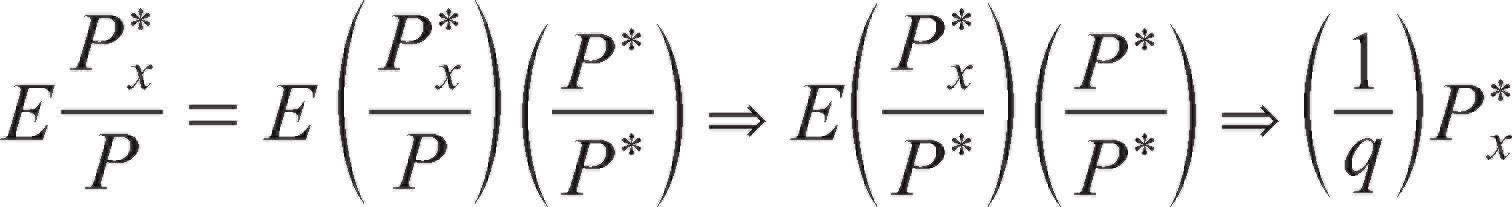
E \frac{P_{x}^{*}}{P} = E (\frac{P_{x}^{*}}{P}) (\frac{P^{*}}{P^{*}}) \Rightarrow E (\frac{P_{x}^{*}}{P^{*}}) (\frac{P^{*}}{P^{*}}) \Rightarrow (\frac{1}{q}) P_{x}^{*}

(4)

Here q denotes the real exchange rate defined as relative price of domestic to foreign goods, $P_{x}^{*}$ is the foreign currency price of foreign country exports and P and P^* are the overall price indices of the home and foreign country, respectively. It may be noted that the real exchange rate so defined (q = P/(E.P^*)) would mean depreciation in case there is a decrease in value of q and vice versa. Using (4) in (3), we get

P_{m} = (\frac{1}{q}) P_{x}^{*}

(5)

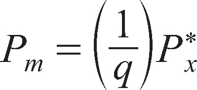
Similarly, foreign import price is defined as

P_{m}^{*} = P_{x} q

(6)

Substituting (5) in (1) and (6) in (2), we get

M_{d} = M_{d} ((\frac{1}{q}) P_{x}^{*}, Y)

(7)

M_{d}^{*} = M_{d}^{*} (P_{x} q, Y^{*})

(8)

Likewise, assuming a perfectly competitive market for export supplies, the domestic (X_s) and foreign export supply $(X_{s}^{*})$ could be expressed as a function of the relative price of exports as

X_{s} = X_{s} (P_{x}) a n d X_{s}^{*} = X_{s}^{*} (P_{x}^{*})

(9)

For the equilibrium condition, we should have equality of demand and supply between exports and imports in each country. That is,

M_{d} = X_{s}^{*} a n d M_{d}^{*} = X_{s}

(10)

On the basis of equation (10) and by using (7) and (8), the domestic trade balance could be expressed as

T B = \frac{X_{s}}{M_{d}} \Rightarrow T B = \frac{M_{d}^{*}}{M_{d}} = {\frac{M_{d}^{*} (P_{x} q, Y^{*})}{M_{d} ((\frac{1}{q}) P_{x}^{*}, Y)}}

(11)

T B = \frac{M_{d}^{*} (P_{x} q, Y^{*})}{M_{d} (\frac{P_{x}^{*}}{q}, Y)}

(12)

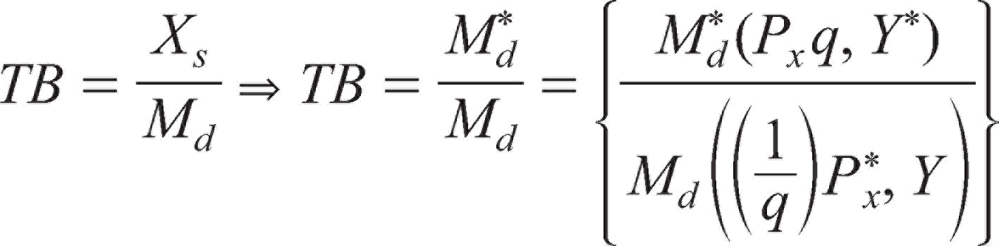
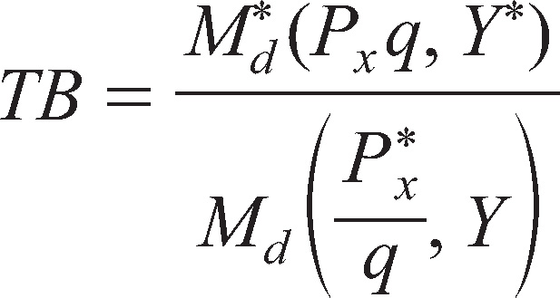
From (12), it can be seen that after solved for the levels of exports and imports along with the relative price ratios, trade balance (TB) can be expressed as a function of q, Y and Y^* as

T B = T B (q, Y, Y^{*})

(13)

Finally from (13), linear estimable function could be expressed in the form of equation (14) as

L n T B_{t} = α + β L n R E E R_{t} + γ L n Y D_{t} + ϑ L n Y F_{t} + μ_{t}

(14)

where TB is defined as $T B_{t} = (\frac{I M P}{E X P})$ . An increase in the ratio denotes a deterioration of trade balance and a decrease connotes an improvement. It is unit free and it measures the trade balance in real terms. The choice of keeping the imports at numerator and exports at denominator is due to the definition of real effective exchange rate (REER) (Bahmani-Oskooee, 1991). According to the construction of REER, a decline in it reflects a real depreciation and to improve the trade balance, the later must be defined as the ratio of imports over exports (Bahmani-Oskooee & Fariditavana, 2015). Therefore, the coefficient β associated with the REER is expected to be positive. YD is supposed to influence the trade balance negatively, that is, γ is expected to be positive. Finally, the expected impact of YF is expected to improve the trade balance and hence ϑ is supposed to be negative.¹²

Econometric Methodology

Equation (14) reflects long-run response of trade balance to changes in explanatory variables and therefore is a static long-run model. The estimates of these models by ordinary least squares may turn out to be spurious if all the variables move together over time and have unit roots. In addition, J-curve is a short-run concept which cannot be tested by a long-run model. To test J-curve effect, some dynamic methods are needed which incorporate both short and long-run relationships.

The traditional definition of the J-curve phenomenon proposed initially by Bahmani-Oskooee (1985) is based on short-run coefficient estimates. Later, Rose and Yellen (1989) suggested an alternative definition of short-run deterioration of trade balance together with a long-run improvement. Various studies judge the J-curve effect as a short-run positive or insignificant coefficient combined with a significant negative long-run coefficient following currency depreciation. To avoid the inadequacy of linear models, an asymmetric cointegration method has been applied to highlight the dynamics of exchange rate and trade balance relationship.

In this study, a non-linear ARDL model developed by Shin et al. (2014) has been used to ascertain the existence of any non-linearities among the variables due to its potential merits over the other conventional linear approaches. It is a convenient approach as it provides a dynamic error correction specification combined with asymmetric long-run cointegration regression by decomposing a given time series w_t into its oppositely signed partial sums ( $w_{t}^{+} a n d w_{t}^{-}$ ) in order to take account of possible asymmetric impact on the dependent variable, x_t. Second, it provides Bounds-based test statistic, used to check for the existence of stable long-run association among variables. Third, the method provides graphs of cumulative dynamic multipliers used to trace out the adjustment patterns following positive and negative shocks to explanatory variables. More importantly, the model permits any asymmetry switching from short run to long run or vice versa.¹³

The asymmetric model developed by Shin et al. (2014) is represented by following error correction specification¹⁴:

Δ x_{t} = γ x_{t - 1} + δ^{+} w_{t - 1}^{+} + δ^{-} w_{t - 1}^{-} + \sum_{i = 1}^{p - 1} π_{i} Δ x_{t - i} + \sum_{i = 0}^{q - 1} (β_{i}^{+} Δ w_{t - i}^{+} + β_{i}^{-} Δ w_{t - i}^{-}) + π_{t}

(15)

where δ⁺ and δ^– are long-run parameters, $β_{i}^{+}$ and $β_{i}^{-}$ represent the short-run asymmetric coefficients and $π_{t} ~ i i d (0, σ_{ω}^{2})$ . The construction of NARDL model in its error correction specification provides a solution for weak exogeneity of any non-stationary independent variable¹⁵ and if the lag structure is correctly chosen, the residual serial correlation is also corrected (Shin et al., 2014).

The empirical procedure of NARDL involves the following steps. First, estimate the ECM as given by equation (15). Second step involves the testing of the presence of cointegration. Shin et al. (2014) provided t_BDM test introduced by Banerjee et al. (1998), tests the null of no cointegration (γ = 0) against an alternative of cointegration (γ ≠ 0) and F_PSS test, advocated by Pesaran et al. (2001), tests the joint null of no cointegration (γ = δ⁺ = δ^– = 0), against an alternative of cointegration (γ ≠ δ⁺ ≠ δ^– ≠ 0). In the final step the short-run and long-run asymmetry is tested by standard Wald’s tests. Equation (15) incorporates the following three possibilities: (i) there exists a long-run symmetry, that is, δ = δ⁺ = δ^– (ii) there exists a short-run symmetry, $\sum_{i = 0}^{q} β_{i}^{+} = \sum_{i = 0}^{q} β_{i}^{-}$ and (iii) there exists a combination of both short- and long-run symmetry.¹⁶

The study finally employs the non-linear cumulative dynamic multipliers to portray the route between disequilibrium position of short period and a new long-run equilibrium of the system. The multipliers highlight the asymmetric adjustment paths and/or duration of disequilibrium. The cumulative dynamic multiplier effects of $w_{t}^{+}$ and $w_{t}^{-}$ on x_t can be evaluated as follows:

l_{h}^{+} = \sum_{i = 0}^{h} \frac{\partial x_{t + i}}{\partial w_{t}^{+}} a n d l_{h}^{-} = \sum_{i = 0}^{h} \frac{\partial x_{t + i}}{\partial w_{t}^{-}}, h = 0, 1

(16)

where $l_{h}^{+}$ and $l_{h}^{-}$ approach towards the respective non-linear steady-state coefficients $α^{+} = \frac{- δ^{+}}{γ} a n d α^{-} = \frac{- δ^{-}}{γ}$ as h → $\infty$ . The segregation about a zero threshold value helps to sketch out the response of dependent variable to positive and negative changes in w_t. These multipliers are derived from the interaction of impact and reaction asymmetries in association with the error correction coefficient γ in equation (15).

So far as the variables incorporated in the study are concerned, we estimate the following model based on equation (15) as

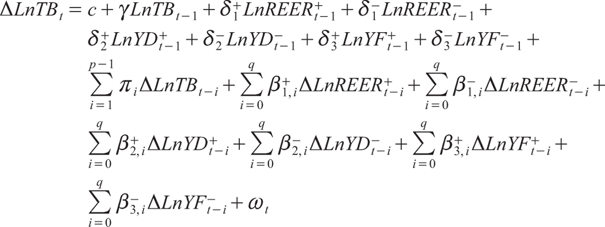
\begin{matrix} Δ L n T B_{t} = c + γ L n T B_{t - 1} + δ_{1}^{+} L n R E E R_{t - 1}^{+} + δ_{1}^{-} L n R E E R_{t - 1}^{-} + \\ δ_{2}^{+} L n Y D_{t - 1}^{+} + δ_{2}^{-} L n Y D_{t - 1}^{-} + δ_{3}^{+} L n Y F_{t - 1}^{+} + δ_{3}^{-} L n Y F_{t - 1}^{-} + \\ \begin{array}{l} \sum_{i = 1}^{p - 1} π_{i} Δ L n T B_{t - i} + \sum_{i = 0}^{q} β_{1, i}^{+} Δ L n R E E R_{t - i}^{+} + \sum_{i = 0}^{q} β_{1, i}^{-} Δ L n R E E R_{t - i}^{-} + \\ \begin{matrix} \sum_{i = 0}^{q} β_{2, i}^{+} Δ L n Y D_{t - i}^{+} + \sum_{i = 0}^{q} β_{2, i}^{-} Δ L n Y D_{t - i}^{-} + \sum_{i = 0}^{q} β_{3, i}^{+} Δ L n Y F_{t - i}^{+} + \\ \sum_{i = 0}^{q} β_{3, i}^{-} Δ L n Y F_{t - i}^{-} + ω_{t} \end{matrix} \end{array} \end{matrix}

(17)

The expected sign of variables incorporated in the analysis is discussed in the section ‘Analytical Framework’. It may be noted that unlike majority of existing empirical studies, we applied a complete asymmetry model. The motivation for choosing such a specification is provided by the various theoretical contours arguing for the existence of asymmetric linkages between dependent variable and various explanatory variables in Section ‘Theoretical Discussion’.

Results and Discussion

To check that none of the variables is I (2), we applied various unit root tests. Table 1 confirms the same and therefore use of NARDL model is validated.¹⁷

Table 1.

Unit Root Analysis

Level	Intercept		Intercept and Trend
Level	ADF Test Stat.	KPSS Test Stat.	ADF Test Stat.	KPSS Test Stat.
LnTB	−1.746 (0.405)	0.439 (0.347)	−1.899 (0.646)	0.194 (0.146)
LnREER	−0.726 (0.883)	1.029 (0.463)	−2.514 (0.321)	0.149 (0.146)
LnYD	0.113 (0.965)	1.197 (0.463)	−1.993 (0.596)	0.193 (0.146)
LnYF	−2.108 (0.242)	1.144 (0.463)	−2.572 (0.294)	0.217 (0.146)
First diff.
ΔLnTB	−4.687 (0.000)*	0.101 (0.347)***	−4.631 (0.002)**	0.102 (0.146)**
ΔLnREE	−9.619 (0.000)*	0.083 (0.463)**	−9.607 (0.000)*	0.055 (0.146)**
ΔLnYD	−4.269 (0.000)*	0.052 (0.463)**	−4.234 (0.006)*	0.052 (0.146)**
ΔLnYF	−5.852 (0.000)*	0.363 (0.463)**	−6.087 (0.000)*	0.133 (0.146)**

Source: Authors calculated.

Note: The corresponding p-values for the ADF test are given in parentheses. However, for the KPSS test, the figures in the parentheses denote the critical values. *, ** and *** denote the statistical significance at 1%, 5% and 10% levels, respectively.

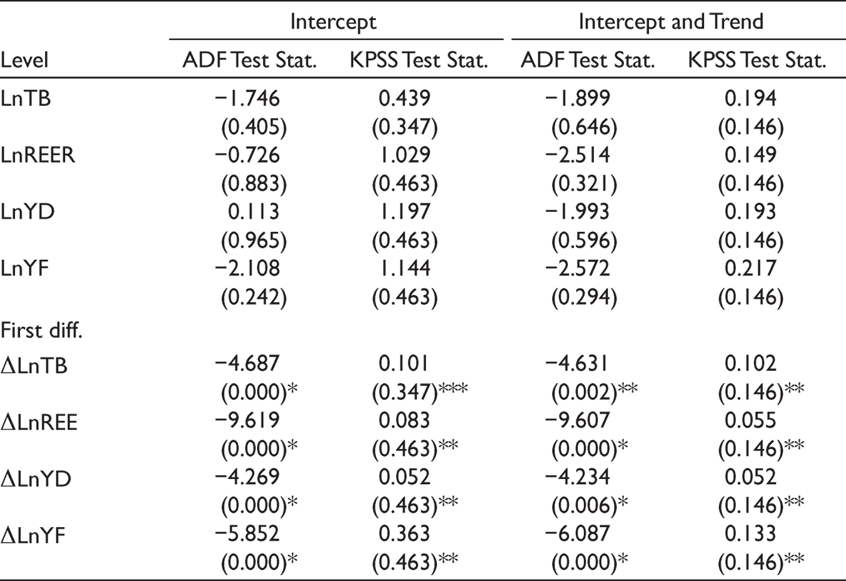
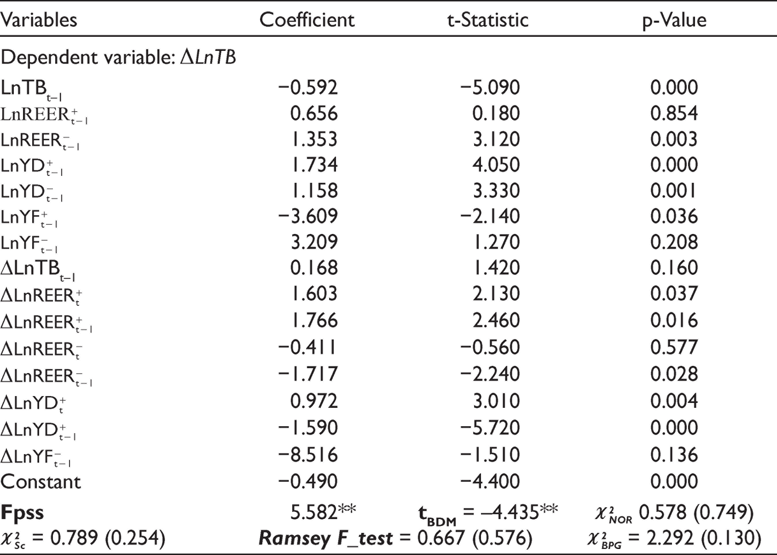
Table 2 documents the results of model (17). A general to specific approach is followed with an initial, lag length of max p = q = 2 is chosen on the basis of AIC and SBC. Subsequently, most of the insignificant lags are excluded to ensure the reliability & avoidance of noise into the dynamic multipliers. The necessary diagnostic tests validating the estimated model are outlined in the lower part of Table 2. The null of no autocorrelation is accepted by portmanteau test $(χ_{S c}^{2})$ , Breusch-Pagan-Godfrey ( $χ_{B P G}^{2})$ test confirms the absence of heteroskedasticity, the structural specification of the model is confirmed by Ramsey RESET test (Ramsey F_test) and finally, the normality requirement of the estimated residuals is reported by the Jarque-Bera ( $χ_{N O R}^{2})$ test.

As can be observed from the lower panel of Table 2, there exists a long-run association among the selected variables since both Fpss and t_BDM are statistically significant at 5 per cent significance level.

We now proceed to test whether cointegration is symmetrical or if some asymmetry is portrayed. Wald’s test with a null of symmetrical association is tested against an alternative of asymmetrical one. As can be observed from Panel B of Table 3, the existence of long-run asymmetrical association is reported between LnTB and all the explanatory variables. In the short run, except between LnTB & LnYF, again the null of symmetrical association is rejected between LnTB and the other two variables. Thus, unlike the previous studies, which confined the existence of asymmetrical impact to the exchange rate only, the present paper established the evidence of the asymmetrical association even in case of other two determinants as well, which validates our full asymmetry model.

Starting with the short-run impact of exchange rate changes on the trade balance, upper panel of Table 2 highlights that while the currency appreciation deteriorates the trade balance in short run, depreciation improves it, although the impact of first lag is statistically insignificant, but the sign implies a favourable impact. Since the impact of most of the lags related to other two variables is statistically insignificant, these are left undiscussed.

Table 2.

Nonlinear ARDL Error Correction Estimation

Variables	Coefficient	t-Statistic	p-Value
Dependent variable: ΔLnTB
LnTB_t–1	−0.592	−5.090	0.000
$L n R E E R_{t - 1}^{+}$	0.656	0.180	0.854
$L n R E E R_{t - 1}^{-}$	1.353	3.120	0.003
$L n Y D_{t - 1}^{+}$	1.734	4.050	0.000
$L n Y D_{t - 1}^{-}$	1.158	3.330	0.001
$L n Y F_{t - 1}^{+}$	−3.609	−2.140	0.036
$L n Y F_{t - 1}^{-}$	3.209	1.270	0.208
DLnTB_t–1	0.168	1.420	0.160
$Δ L n R E E R_{t}^{+}$	1.603	2.130	0.037
$Δ L n R E E R_{t - 1}^{+}$	1.766	2.460	0.016
$Δ L n R E E R_{t}^{-}$	−0.411	−0.560	0.577
$Δ L n R E E R_{t - 1}^{-}$	−1.717	−2.240	0.028
$Δ L n Y D_{t}^{+}$	0.972	3.010	0.004
$Δ L n Y D_{t - 1}^{+}$	−1.590	−5.720	0.000
$Δ L n Y F_{t - 1}^{-}$	−8.516	−1.510	0.136
Constant	−0.490	−4.400	0.000
Fpss	5.582**	t_BDM = –4.435**	$N O R_{}^{2}$ 0.578 (0.749)
$S c_{}^{2}$ = 0.789 (0.254)	Ramsey F_test = 0.667 (0.576)		$B P G_{}^{2}$ = 2.292 (0.130)

Source: Authors calculated.

Note: Fpss and t_BDM are the long-run cointegration tests and ** denotes significance at 5%.

In the long run, the Panel A of Table 3 highlights the statistically insignificant deterioration of trade balance following an appreciation and a statistically significant improvement following a depreciation. The outcome of this result at the outset provides an indication that the J-curve phenomenon is not observed in case of India either according to traditional definition (Bahmani-Oskooee, 1985) or according to the definition given by Rose and Yellen (1989).¹⁸ Secondly, incorporating the asymmetrical framework, it is found that effect of depreciation is more than appreciation, although the latter is statistically insignificant. A 1 per cent increase in exchange rate is found to deteriorate the trade balance by around 0.111 per cent and a decrease in it by an equal magnitude leads to an improvement in trade balance by around 2.286 per cent. The channels discussed in the section ‘Theoretical Discussion’ offer possible explanations for the existence of asymmetric effects of the exchange rate on the trade balance.

Table 3.

Long-Run and Short-Run Asymmetric Tests and Effects

PANEL_A	Long-Run Effect [+]			Long-Run Effect [–]
Variables	Coef.	F-Stat	P-Value	Coef.	F-Stat	p-Value
LnREER	0.111	0.351	0.852	−2.286	22.22	0.000
LnYD	2.929	18.52	0.000	−1.956	2.796	0.003
LnYF	−6.094	5.547	0.021	−5.420	1.724	0.194

PANEL_B	Long-Run Asymmetry		Short-Run Symmetry
	Long-Run W LR		Short-Run WSR
	F-Statistic	p-Value	F-Statistic	P-Value
LnREER	15.48	0.000	10.97	0.001
LnYD	5.127	0.027	2.796	0.099
LnYF	3.518	0.065	2.281	0.136

Source: Authors calculated.

Coming to the impact of domestic demand changes, an increase in it deteriorates trade balance and a fall improves it. However, again an asymmetry is reported and effect of increase in domestic demand is more in magnitude than due to the decrease in it. The results are, however, contrary to what should have been the case following the earlier studies. The outcome of this result could possibly be attributed to presence of a strong consumer base in India, the existence of capital constraints in the production chain and the presence of huge import bill which continues even in the depressed demand conditions (Bhat et al., 2018). Any augmentation in the domestic demand would mean an additional pressure on the existing capital base which is already facing constraints, an increase in the costs of production, an increased demand for oil & other imports. Thus, imports are swallowing very heavily, but due to the inability to supply to both the markets and due to excessive pressure domestically, exports are not increased and the impact on trade balance would be detrimental. On the contrary, if the domestic demand falls, its negative effect on the imports (mostly intermediate in nature) is very meagre since these continue to grow even in the depressed demand conditions and due to existence of little excess capacity in the manufacturing units, exports may increase but only marginally. Therefore, the improvement in trade balance following a decline in domestic demand conditions is relatively low.

Finally, 1 per cent increase in foreign demand improves the trade balance by 6.094 per cent and the impact of a decline is statistically insignificant. The positive response of trade balance to an increase in the foreign demand follows Keynesian orthodoxy whereby a hike in later leads to stimulation of domestic exports to the rest of world and if the demand for imports remains unchanged, the trade balance improves. However, the statistical insignificance of negative demand shock personifies the consumption downward inflexibility.

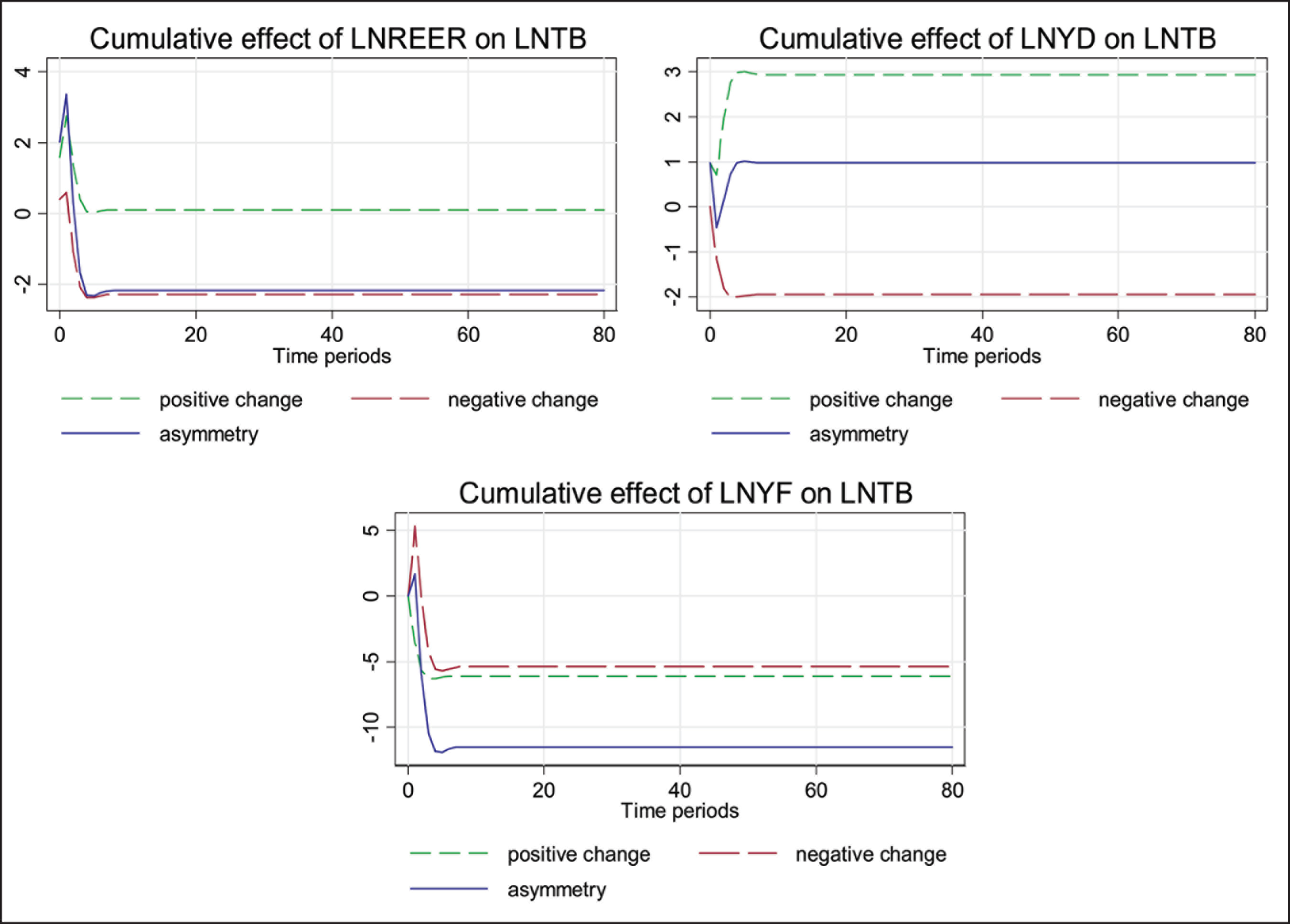
To ensure the robustness, dynamic multipliers, as depicted in Figure 1, connote the impact of explanatory variables on the trade balance of India. A synoptic view confirms what has already been discussed. The blue line indicates the extent of asymmetry at any point. Moreover, it takes around 5 quarters on average to reach to new equilibrium position following any short-run disturbance.

Figure 1.

Source: Authors calculated.

Conclusion

This paper examines the asymmetric impact of exchange rate changes on the trade balance of a developing country, namely, India. Using NARDL model, evidence in favour of short and long-run asymmetry has been reported. Currency appreciation is found to deteriorate the trade balance in short run; however, depreciation improves it. In the long run, we found a statistically insignificant deterioration of trade balance following an appreciation and a statistically significant improvement following depreciation. The outcome of this result refutes the J-curve phenomenon in case of India. The effect of depreciation is more than the appreciation. It appears that the Marshal–Lerner condition holds in long run and country benefits from rupee depreciation. Similarly, the impact of domestic demand on the trade balance is reported to be deleterious. However, again an asymmetry is observed whereby an increase in domestic demand deteriorates it by a greater magnitude than an improvement is observed due to a fall in domestic demand. Finally, increase in foreign demand is found to improve the trade balance relatively by a higher percentage than is observed due to decline in it.

The outcome of these results leads to some intuitive policy implications. Even though, foreign demand is exogenous to Indian policy making, however, special initiatives to improve the external competitiveness to attract the foreign demand could be implemented. Secondly, the economy should develop sufficient productive capacity to lower its dependence on the imports during increased demand conditions. The increased productive capacity will also enable the domestic capital constrained firms to expand the export baskets and substitute the domestic demand with the foreign sales and thereby prove an additional channel to avoid the repercussions of declining demand. Finally, even though currency depreciation improves the trade balance, but it should not be resorted as a routine channel to achieve a competitive external position at the cost of the exchange rate misalignment and/or deficit persistence in the current account.

The policy stance related to the exchange rate is a bit tricky in India. Although the monetary authorities have no explicit policy target about the exchange rate, however, it justifies its intervention to lower the exchange rate volatility.¹⁹ Moreover, in the earlier times, exchange rate was determined solely by the level of current account deficit because the level of capital inflows was very grim and passive, but that is not true in the contemporary times. With the inflows exceeding the current account deficit, nominal exchange rate may remain same or may even appreciate. More particularly, at that time, if the domestic inflation is higher than that of trading partners, the real exchange rate will appreciate. If appreciation of nominal exchange rate is prevented through the central bank intervention by buying the excess foreign currency, but in the real terms exchange rate may appreciate if the additional reserves so accumulated lead to an increase in money supply well above the desired targets and hence lead to price hikes. If the central bank is interested to eliminate the impact of additional reserves on the domestic money by issuing the bonds to absorb the excess liquidity out of the system, but a cost to it is a function of rate of returns to reserves and the interest on stabilisation bonds.

India does have a large trade deficit, even though overall current account deficit is low because of the surplus on the services account. With the capital inflows playing an important role in the exchange rate determination, it would be imperative to offset the influence of capital inflows in order to avoid the real appreciation of domestic currency, which otherwise would erode the competitiveness of the Indian exports. Moreover, since the nominal depreciation has an effect on capital inflows, foreign investors would only be willing to invest in a country only if they are provided a higher rate of return in currency depreciating country.²⁰ Thus, the obvious implications of exchange rate depreciation on the capital inflows and the resulting macroeconomic ramifications need to be addressed with extra emphasis. In addition, the stability of domestic prices plays a crucial role in maintaining the exchange rate stability, therefore, a monetary policy framework designed to ensure price stability is highly warranted.

Footnotes

Declaration of Conflicting Interests

The authors declared no potential conflicts of interest with respect to the research, authorship and/or publication of this article.

Funding

The authors received no financial support for the research, authorship and/or publication of this article.

Notes

References

Arize

A. C.

, & Darrat

A. F.

(1994). The value of time and recent US money demand instability. Southern Economic Journal, 60, 564–578.

Arize

A. C.

, & Malindretos

(2012). Nonstationarity and nonlinearity in inflation rate: Some further evidence. International Review of Economics & Finance, 24, 224–234.

Arize

A. C.

, Malindretos

, & Igwe

E. U.

(2017). Do exchange rate changes improve the trade balance: An asymmetric nonlinear cointegration approach. International Review of Economics & Finance, 49, 313–326.

Aziz

(2008). The role of exchange rate in trade balance: Empirics from Bangladesh. University of Birmingham.

Bahmani-Oskooee

(1985). Devaluation and the J-curve: Some evidence from LDCs. The Review of Economics and Statistics, 67(3), 500–504.

Bahmani-Oskooee

(1991). Is there a long-run relation between the trade balance and the real effective exchange rate of LDCs? Economics Letters, 36(4), 403–407.

Bahmani-Oskooee

(2001). Nominal and real effective exchange rates of Middle Eastern countries and their trade performance. Applied Economics, 33(1), 103–111.

Bahmani-Oskooee

, Aftab

, & Harvey

(2016). Asymmetry cointegration and the J-curve: New evidence from Malaysia-Singapore commodity trade. The Journal of Economic Asymmetries, 14, 211–226.

Bahmani-Oskooee

, & Baek

(2016). Do exchange rate changes have symmetric or asymmetric effects on the trade balance? Evidence from US–Korea commodity trade. Journal of Asian Economics, 45, 15–30.

10.

Bahmani-Oskooee

, & Fariditavana

(2015). Nonlinear ARDL approach, asymmetric effects and the J-curve. Journal of Economic Studies, 42(3), 519–530.

11.

Bahmani-Oskooee

, & Fariditavana

(2016). Nonlinear ARDL approach and the J-curve phenomenon. Open Economies Review, 27(1), 51–70.

12.

Bahmani-Oskooee

, Harvey

, & Hegerty

S. W.

(2017). The Japanese trade balance and asymmetric effects of yen fluctuations: Evidence using nonlinear methods. The Journal of Economic Asymmetries, 15, 56–63.

13.

Bahmani-Oskooee

, & Hegerty

S. W.

(2010). The J- and S-curves: A survey of the recent literature. Journal of Economic Studies, 37(6), 580–596.

14.

Balke

N. S.

, & Fomby

T. B.

(1997). Threshold cointegration. International Economic Review, 38(3), 627–645.

15.

Bhat

J. A.

, Ganaie

A. A.

, & Sharma

N. K.

(2018). Macroeconomic response to oil and food price shocks: A structural var approach to the Indian economy. International Economic Journal, 32(1), 66–90.

16.

Cheung

Y. W.

, & Sengupta

(2013). Impact of exchange rate movements on exports: An analysis of Indian non-financial sector firms. Journal of International Money and Finance, 39, 231–245.

17.

Dickey

D. A.

, & Fuller

W. A.

(1979). Distribution of the estimators for autoregressive time series with a unit root. Journal of the American Statistical Association, 74(366a), 427–431.

18.

Hatemi-J

, & Irandoust

(2005). Bilateral trade elasticities: Sweden versus her major trading partners. American Review of Political Economy, 3(2), 38–50.

19.

Kishore Sahoo

, Nauriyal

D. K.

, & Mohapatar

(2015). Software exports from India: An econometric exploration. Journal of Asia-Pacific Business, 16(4), 274–301.

20.

Korkmaz

, & Bilman

M. E.

(2017). The S-curve behaviour of the trade balance: A stepwise procedure. Foreign Trade Review, 52(1), 1–14.

21.

Liew

K. S.

, Lim

K. P.

, & Hussain

(2000). Exchange rate and trade balance: The experience of ASEAN countries. Journal of Management Sciences, 3, 15–18.

22.

Magee

S. P.

(1973). Currency contracts, pass-through, and devaluation. Brookings Papers on Economic Activity, 1973(1), 303–325.

23.

Pesaran

M. H.

, Shin

, & Smith

R. J.

(2001). Bounds testing approaches to the analysis of level relationships. Journal of Applied Econometrics, 16(3), 289–326.

24.

Psaradakis

, Sola

, & Spagnolo

(2004). On Markov error-correction models, with an application to stock prices and dividends. Journal of Applied Econometrics, 19(1), 69–88.

25.

Rajan

R. S.

, & Yanamandra

V. R.

(2015). Managing the macroeconomy: Monetary and exchange rate issues in India. Springer.

26.

Rangarajan

, & Kannan

(2017). Determinants of India’s exports. Journal of Quantitative Economics, 15(3), 629–646.

27.

Rose

A. K.

, & Yellen

J. L.

(1989). Is there a J-curve? Journal of Monetary Economics, 24(1), 53–68.

28.

Roy

S. S.

(2007). Demand and supply factors in the determination of India’s disaggregated manufactured exports: A simultaneous error-correction approach. Centre for Development Studies.

29.

Sharma

(2003). Factors determining India’s export performance. Journal of Asian Economics, 14(3), 435–446.

30.

Shin

, Yu

, & Greenwood-Nimmo

(2014). Modelling asymmetric cointegration and dynamic multipliers in a nonlinear ARDL framework. In Festschrift in Honor of Peter Schmidt (pp. 281–314). Springer.

31.

Shirvani

, & Wilbratte

(1997). The relationship between the real exchange rate and the trade balance: An empirical reassessment. International Economic Journal, 11(1), 39–50.

32.

Singh

(2002). India’s trade balance: The role of income and exchange rates. Journal of Policy Modeling, 24(5), 437–452.

33.

Sun

C. H.

, & Chiu

Y. B.

(2010). Taiwan’s trade imbalance and exchange rate revisited. Applied Economics, 42(7), 917–922.

34.

Tandon

(2014). Trade balance and the real exchange rate: An empirical analysis of multilateral and bilateral relationship. Foreign Trade Review, 49(2), 117–139.

35.

Thomas

M. P.

(2016). Estimation of income and price elasticities of India’s trade in services: Evidence from Post-WTO period. South Asia Economic Journal, 17(1), 27–45.

36.

Upadhyay

, & Ghosh Roy

(2016). Impact of exchange rate movement and macro-economic factors on exports of software and services from India. Benchmarking: An International Journal, 23(5), 1193–1206.

37.

Veeramani

(2007). Sources of India’s export growth in pre-and post-reform periods. Economic and Political Weekly, 42(25), 2419–2427.

38.

Veeramani

(2008). Impact of exchange rate appreciation on India’s exports. Economic and Political Weekly, 43(22), 10–14.

39.

Wilson

, & Tat

K. C.

(2001). Exchange rates and the trade balance: The case of Singapore 1970 to 19961. Journal of Asian Economics, 12(1), 47–63.