
Abstract
The purpose of the article is to find the effect of public expenditure (GI) and private project expenditure (PI) in different states on state gross domestic product (SGDP) and national gross domestic product (NDGP). The study also attempts to examine the sectors that contribute the most in growth of state and nation. The selected sectors in the study include manufacturing, mining, services, power, construction and infrastructure and irrigation. Data of all states and four union territories (UTs) for GI and PI in selected sectors are collected and a panel is formed. Four different regression equations are developed. The estimation is done using two-step Arellano–Bover/Blundell–Bond’s dynamic panel data to account for endogeneity and heteroscedasticity. The results suggest there exist two clusters of states in India. First cluster is of 13 states, which contributes towards the economic growth of nation and the other cluster is 16 states and UTs that do not contribute towards the economic growth of nation. The states that contribute towards the economic growth of nation do it primarily through private investment in the service sector.
Keywords
Introduction
The theories of economic growth have evolved over time. However, despite centuries of research, the questions like ‘What are the determinants of economic growth?’ and ‘Does economic growth lead to welfare of a state and the nation as a whole?’ are still relevant today. Economic growth, which is generally measured as the increase of real gross domestic product (GDP) or GDP per capita, gets directly influenced by factors like the use of human resources and natural resources (land, underground resources) and the increase in capital employed or technological advancements (Denison, 1962). Economic growth is also indirectly affected by factors such as institutions (financial institutions, private administrations etc.), the size of the aggregate demand, saving rates and investment rates, the efficiency of the financial system, budgetary and fiscal policies, migration of labour and capital and the efficiency of the government (Boldeanu & Constantinescu, 2015). Apart of these, socio-political factors, regional politics, and geographical location of a state/nation also influence the economic growth of a nation.
The public (government expenditure) and private project expenditure play a vital role in economic growth. However, researchers in the past provided contradicting evidences. Most of the studies that have examined the role of public expenditure (GI) and private project expenditure (PI) on economic growth are primarily cross-country comparisons and draw conclusions from bi-variate analysis. Hence, such studies suffer from the omission of variables (Sehrawat & Giri, 2015). Further, to the best of author’s knowledge, studies have not examined the impact of GI and PI on states within a nation. Therefore, it is important to explore, how GI and PI within states contribute to the economic development of states as well as the nation and how successful the states are in terms of their ability to transfer benefit of this expenditure towards economic growth.
Researchers in the past have attempted to examine interstate disparities in India (Ahluwalia, 2000; Bandhopadhyay, 2012; Kalra & Thakur, 2015; Kaur & Kaur, 2016; Trivedi, 2002). In a study on selected 15 states, Mallick (2013a) finds that there is a high variation in the private project investment across Indian states. Rey and Montouri (1999), Rey (2001) and Janikas and Rey (2005) examine the interstate disparities in USA. Gallo (2004), Dall’erba and Gallo (2008), Dall’erba et al. (2008), Maza and Villaverde (2009) and Rey and Sastre´-Gutie´rrez (2010) examined the same in Europe.
As noted, researchers in the past have examined interstate disparities, with no focus on how successful these states are in transferring the benefit of public and private capital expenditure towards economic growth of nation. To some extent, Mallick (2013b) and Murova and Khan (2017) investigate these issues in India and USA, respectively, but on a smaller sample. The current study, therefore, is an attempt to examine the issues of GI and PI, by using multivariate analysis with the help of time series data, in India at the state level for all 29 states and four union territories (UT)s. Hence, the proposed study tries to understand: whether the growth in state gross domestic product (SGDP) leads to the growth in national gross domestic product (NGDP); the role of growth in GI and PI towards the growth of SGDP and NGDP; and the influence of specific sectors on SGDP and NGDP.
The rest of the study is divided into four sections. The next section is literature review that discusses the impact of public and private project expenditure on economic growth of a nation and the role of sector specific investment in achieving economic growth. Section three is research methodology that explains the procedure adopted followed by preliminary data investigation and model development and testing. Finally, the study is concluded with summary of results and discussion.
Literature Review
The importance of government intervention in economic growth has been debated since centuries, with one extreme view of liberalism and the other of Marxist’s state control. John Maynard Keynes seemed to offer a middle path with the role of government intervention, only when needed. During the early days after independence, India followed a mixed approach with higher government intervention and reduced role of private investment.
However, things changed after 1991–1992. India witnessed its worst balance of payment crisis in 1991, and this resulted in a policy shift and opening up of economy through the gradual shift towards liberalisation, privatisation and globalisation with increased role of private sector project expenditure. Now, the GI is restricted to few sectors. This shift in the economic policy is accompanied by empirical evidences that range from studies on the importance of GI and PI in infrastructure, health and education.
Public Project Expenditure and Economic Growth
Afonso and Furceri (2010), Al-Yousif (2000), Barro (1990), Chamorro-Narvaez (2012), Folster and Henrekson (2000), Haque (2004), Gallaway and Vedder (1998), Gupta et al. (2005), Ghosh and Gregoriou (2008), Gwartney et al. (1998) and Yilmaz (2018) have examined the relationship between GI and economic growth of a nation. Easterly and Rebelo (1993) and M’Amanja and Morrissey (2004) report a positive relation between GI and economic growth, while several others such as studies by Barro (1990), and Cashin (1995) or no relation by Kormendi and Meguire (1985) and Poot (2000) find a negative relation. Soli et al. (2008), in a study in Ghana, suggest the increasing importance of PI in economic growth.
Public Project Expenditure in Infrastructure Sector and its Impact on Economic Growth
The GI in infrastructure sector, such as transportation, healthcare, education and natural resources, does play a vital role in the economic growth of the state as well as the nation. León-González and Montolio (2004), Pereira and Andra (2005), Shioji (2001) examined the impact of investment made in infrastructure transport facilitates by way of GI and found a significant impact. Similarly, GI made in public health and education spending had a significant effect on economic growth of a nation (Bose, et al., 2007; Easterly & Rebelo, 1993; Odedokun, 2001; Ramirez & Nazmi, 2003).
Babatunde (2018) indicates that government spending on transport and communication and education and health infrastructure has significant effects on economic growth; spending on agriculture and natural resources infrastructure recorded a significant inverse effect on economic growth in Nigeria. In a convergence model approach, using a panel data for the USA and a few Japanese regions for the year 1963–1993, Shioji (2001) find that infrastructure project has a significant positive linkage with economic growth. On the contrary, Ashauer (1989) and Holtz-Eakin and Schwartz (1995) find no or only marginal impact of infrastructure investments (both public and private) on economic growth. Nijkamp and Poot (2004), in their study, conclude that public infrastructure together with education promotes economic growth. Mallick and Mahalik (2010) find that, in India, economic growth would continue to decline if there exists capital deepening (capital intensity) alone without reasonable technological progress and if inefficient utilisation of capital and wear and tear charges continue.
Private Project Expenditure in Infrastructure Sector and Its Impact on Economic Growth
Few studies report the effect of private project expenditure on economic growth (Ahluwalia, 2000; Baddeley et al., 2006; Blejer & Khan, 1984; Everhart & Sumlinski, 2001; Khan & Reinhart, 1990; Krishna, 2004; Odedokun, 1997; Rao et al., 1999). Rao et al. (1999), Baddeley et al. (2006) and Purfield (2006) show the positive association between PI and economic growth. Makuyana and Odhiambo (2017) report that productivity of GI and PI in Zimbabwe can be improved by cutting on non-infrastructural public investment to basic minimum level while stimulating the growth in infrastructural public investment. Makuyana and Odhiambo (2018) find that PI has a positive impact on economic growth both in the long run and short run, while GI has a negative effect on economic growth in the long run. Chotia and Rao (2018), in their study, find that infrastructure projects in the area of roads, seaports, telecommunication and energy, if funded by private sector, will lead to economic growth of India. Nguyen and Trinh (2018) suggest that investment from the private sector has positive effects on short-term economic growth.
Overall, there are a lot of studies that explain the significant positive/negative effect of GI and PI on economic growth of a nation with cross-country comparison. Further, studies about sectors that contribute towards the economic growth are available. Most of these studies have used standard time series regression analysis or panel regression methods depending on the need and nature of data. However, the studies looking into regional aspects of a nation and digging deeper to find the impact of GI and PI on economic growth of a state/region as well a nation are almost non-existent.
Research Methodology
About Indian States
India is a huge and a complex nation with 29 states and 7 union territories (UT). Some of the states are bigger in terms of the geographical area and population and others are relatively smaller. Even the climatic conditions and terrain differ from state to state. Some states have abundance of natural resources while others have none. Few states have huge water resources while others strive for water. States in the North-East and the Leh Ladakh region are not even well connected to the rest of the country. These differences in the states lead to regional disparities and a huge difference in SGDP. Central government initiates different development schemes in the form of GI in all the states, depending on their needs and keeping in mind their regional advantages and disadvantages. These investments are made in different types of projects such as power, irrigation, manufacturing, services, mining, construction and infrastructure. Some of these projects are also funded through state budgets, but most are centre-funded and the balance need is financed through PI. PI play a vital role in this development process, and states that are able to provide a conducive environment for private project expenditure attract huge private investment.
Data and Variables
Variable Identification

Variable Identification
The data for a period of 17 years (2002–2018) for 29 states and 4 UTs as well as India as a whole were collected except for 3 UTs, namely Dadra and Nagar Haveli, Daman and Diu and Lakshadweep because of non-availability of data. SGDP and NGDP are dependent variables and PI and GI are primary independent variables. MF, MI, PW, SER, CON and IRR are subsectors of PI and GI. The definition of these variables is provided in Table 1. However, the data with regard to how much investment in each sector has come from PI and GI source are not available. A strongly balanced panel of this data is created. GI includes the funds allocated by the central government for different projects across states and PI includes funds sourced from both the domestic and foreign investors in the form of foreign direct investment. MF includes projects in the area of food and agro-based products, textile, chemicals, consumer goods, construction material, mettles, machinery and transport equipment. SER includes project investment in hotels, tourism, hospitals and schools, communication and trade, whereas CON includes projects in roads, rails, bridges, flyovers, real estate, etc.
Correlation Matrix
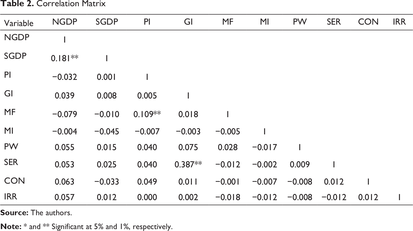
Correlation Matrix
Im–Pesaran–Shin Unit-root Test

Based on the results of multicollinearity and stationarity and considering the data is a balanced panel, four different panel regression equations are developed. The panel regression equation differs from a regular time series or cross-section regression by the double subscript attached to each variable (Amidu & Abor, 2006).


here i denotes the cross-sectional dimension and t represents the time series dimension. αi is constant over time and specific to an individual cross-section state i. β is the coefficient of explanatory variable and ε is an error or residual. The two dependent variables are SGDP and NGDP, where SGDP represents the growth in state GDP and NGDP represents growth in nations GDP. PI is growth in private project investment in a state (inclusive of foreign direct investment), GI is growth in government (public) project investment in a state, MF is growth in investment in manufacturing sector in a state, MI is growth in investment in mining sector in a state, PW is growth in investment in power sector in a state, SER is growth in investment in service sector in a state, CON is growth in investment in construction sector in a state and IRR is growth in investment in irrigation sector in a state. These equations have been developed based on their theoretical relationship that has been discussed in literature review.
Before, we proceed for the model testing, the initial models are tested for heteroscedasticity using Breusch–Pagan/Cook–Weisberg test for heteroscedasticity. The null hypothesis of constant variance for each model and chi-square (χ2) value and p-values of each model are 2.19 (0.1393), 0.04 (0.8346), 0.41 (0.5195) and 0.67 (0.4117), respectively, hence the models do not suffer from the problem of heteroscedasticity.
Endogeneity in regression models refers to the condition in which an independent variable in the model correlates with the residual term, which potentially leads to wrong inferences, misleading conclusions and incorrect theoretical interpretations (Singla, 2020; Ullah et al., 2018). In such cases, the researchers might not get the correct sign of coefficients (Ketokivi & McIntosh, 2017). Ullah et al. (2018) suggest that the Arellano–Bover/Blundell–Bond’s dynamic panel data estimator can be used in all such cases. Further, Ketokivi and McIntosh (2017) point that the error term in endogeneity bias is unobservable, so there is no direct way to statistically test that an endogenous variable is correlated with the error term and it is therefore almost impossible to statistically ensure that an endogeneity problem can be completely resolved (Roberts & Whited, 2012). Therefore, Ketokivi and McIntosh (2017) recommend the use of better choice of model. Arellano and Bond (1991) and Blundell and Bond (1998) developed the generalized method of moments (GMM) model, which can be used for dynamic panel data. The model includes lagged values of dependent variable and first (one step) or second level (two step) of transformed data. Hence, this provides consistent results in the presence of different sources of endogeneity, namely ‘unobserved heterogeneity, simultaneity and dynamic endogeneity’ (Wintoki et al., 2012, p. 588).
Average State-wise Growth in Study Variables During 2002–2018
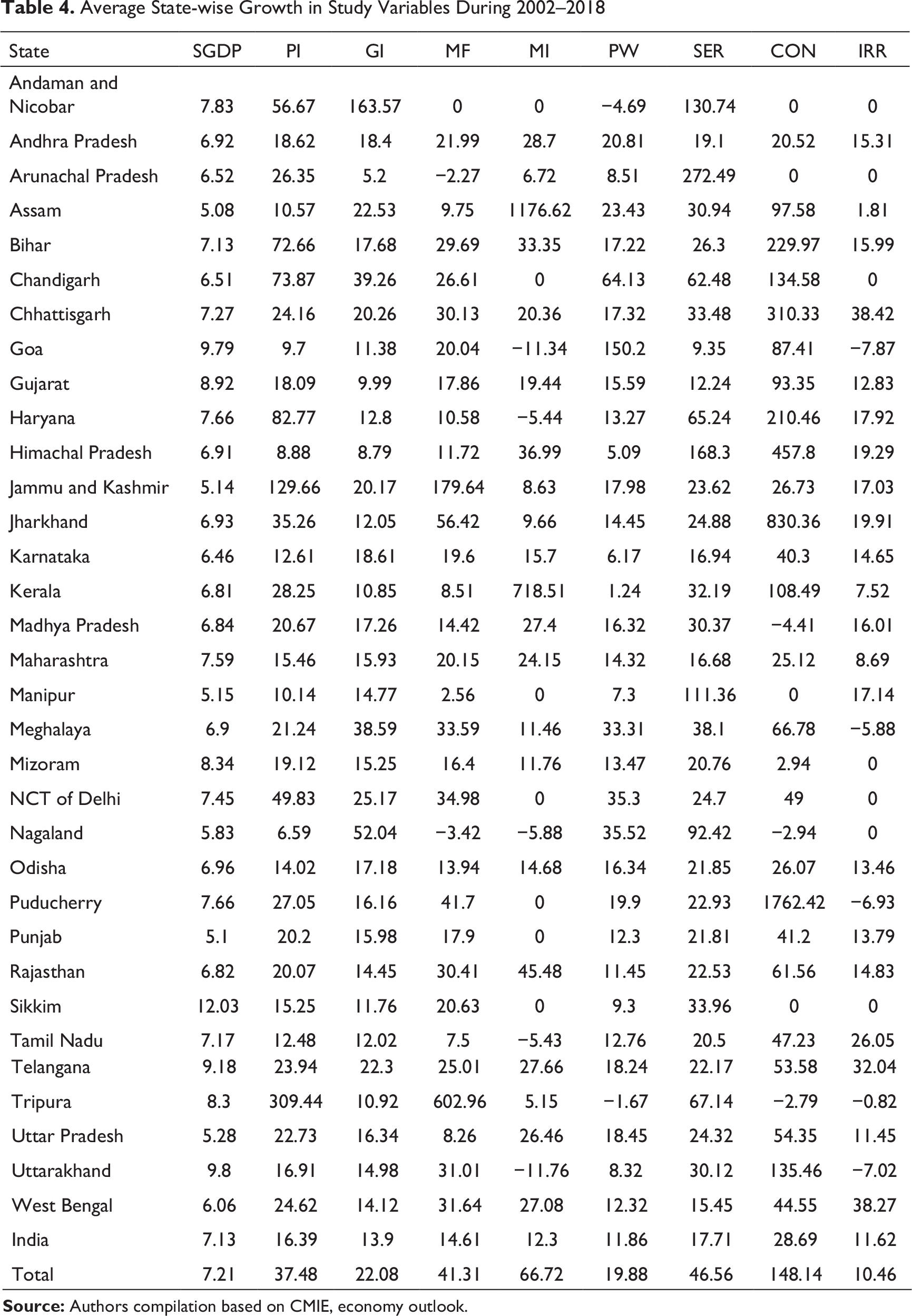
Average Growth in Study Variables

Average Growth in Study Variables
The results of Table 4 indicate that Sikkim recorded the highest growth in SGDP (12.03%), the only state to record a double-digit growth. The other states that are showing a decent growth are Goa (9.79%), Telangana (9.18%), Gujrat (8.92%) and Mizoram (8.34%). The states with relatively lower growth are Assam (5.08%), Manipur (5.15%), Punjab (5.1%), Jammu and Kashmir (5.14%) and Uttar Pradesh (5.28%). The PI grew in Tripura by 309.44 per cent and in Jammu and Kashmir by 129 per cent, which is huge; however, it is interesting to note that despite such huge growth in PI, these states do not record very high SGDP. The other states that recorded higher PI are Haryana, Bihar and Chandigarh. Small states like Goa and Himachal Pradesh recorded slow growth in PI. The GI grew highest in Andaman & Nicobar (163%). Chandigarh (39.26%), Meghalaya (38.59%) and Nagaland (52.04%) had decent growth in GI.
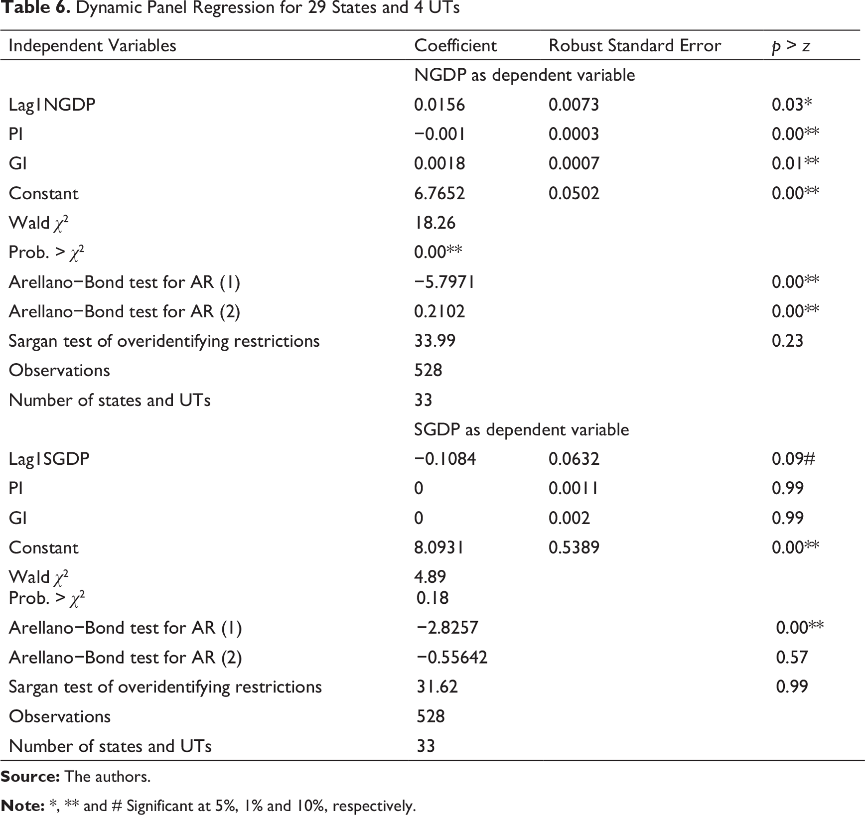
Dynamic Panel Regression for 29 States and 4 UTs
Dynamic Panel Regression for 29 States and 4 UTs: Sector Specific Project Investment

The results for overall panel in Table 6 show that PI negatively affects the NGDP, whereas GI affects NGDP positively. SGDP is not affected by both GI and PI. There is a significant lag effect in both the models. The first equation is significant (p < α at 0.05 = 0.00 and Wald χ2 is 18.26), while the second is not significant (p > α at 0.05 = 0.18 and Wald χ2 is 4.89). In order to examine the diagnosis of GMM, serial correlation is tested using the Arellano–Bond test, and overidentification is tested by Sargan (1958)’s test of over-identifying restrictions. The diagnostic tests for NGDP reveal that there is a first and second order autocorrelation in the disturbances of the first-difference equations for GMM at 1 per cent significance level. However, for the Sargan test of overidentification, the null hypothesis of ‘overidentifying restrictions are valid’ is accepted. On the other hand, the diagnostic tests for SGDP reveal that there is a no second-order autocorrelation in the disturbances at 1 per cent significance level and the null hypothesis of ‘overidentifying restrictions are valid’ is also accepted.
The results in Table 7 show that investment in service and irrigation sector positively affects the NGDP, whereas investment in manufacturing sector has a negative influence on SGDP. The third equation is significant (p < α at 0.05 = 0.00 and Wald χ2 is 26.18), but the fourth equation is not significant (p > α at 0.05 = 0.16 and Wald χ2 is 10.45). Overall, both equations based on NGDP are significant, while equations based on SGDP are insignificant.
In order to further investigate, authors decided to study each state separately using times series Equations (5)–(7). This is because the earlier results can be biased due to of the presence of all the states in the panel, irrespective of their nature, size and geographical advantage/disadvantage.


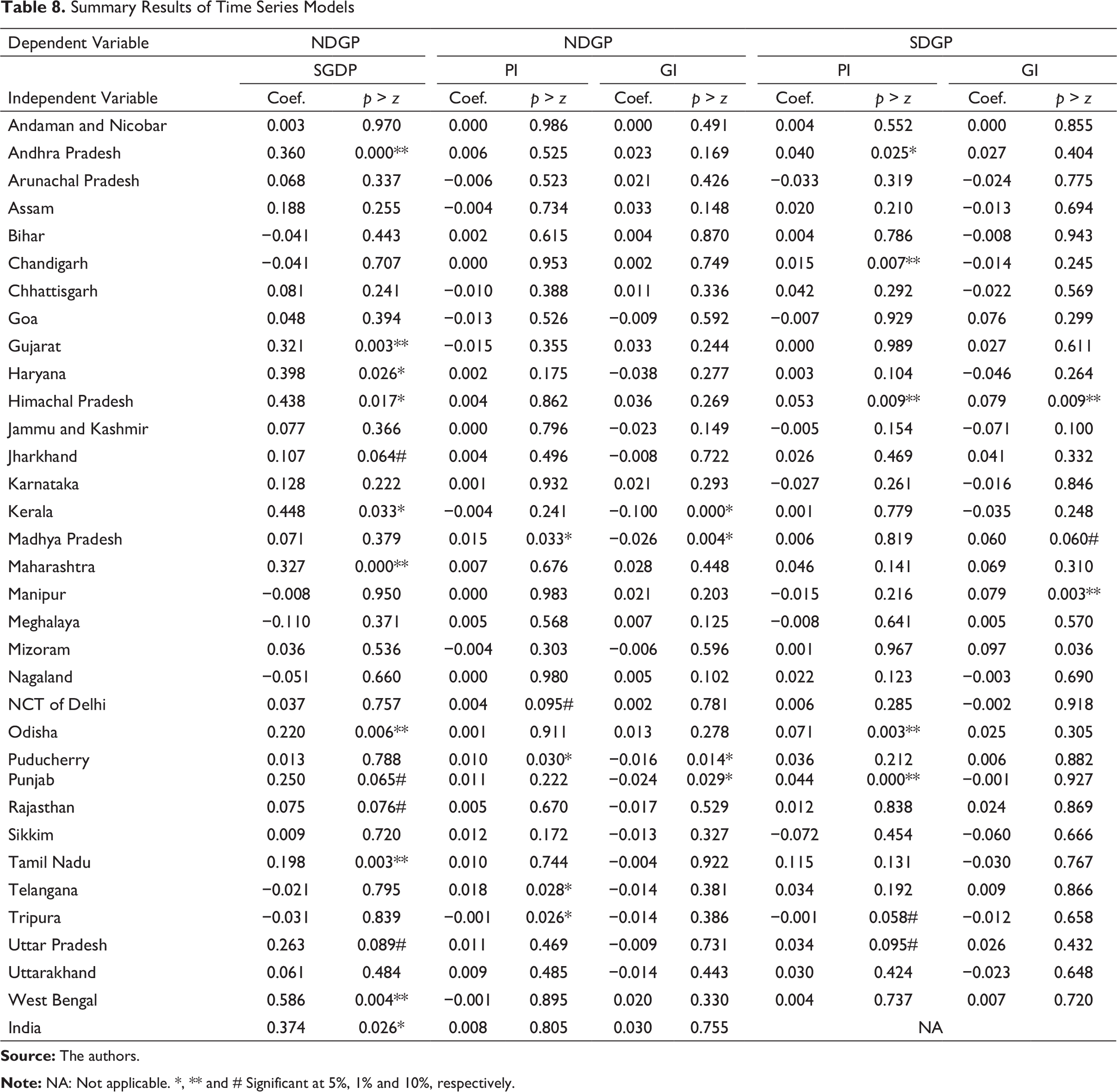
The results in a summary form are presented in Table 8.
The results in Table 8 give a clear view and show that in 13 states, the SGDP positively drives the NGDP. This suggests that these states are directly influencing the NGDP. In the remaining 16 states and 4 UTs, the SGDP is not driving the NGDP. Private investment has positive influence on SGDP for six states and four states for NGDP with only exception of Tripura, which is showing a negative effect. Based on these results, authors decided to divide the panels into two clusters. First cluster is a panel of 13 contributing states and other panel is of 16 non-contributing states and 4 UTs. The results of these panels estimated for Equations (1)–(4) are presented in Tables 9–12.
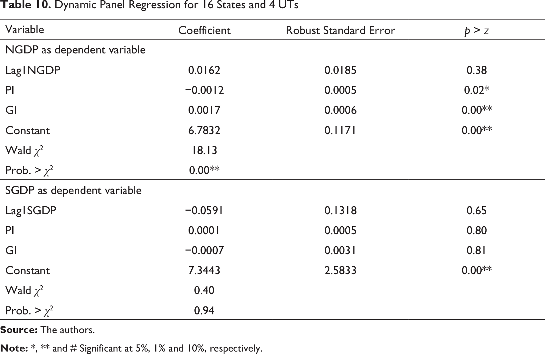
The results of Tables 9 and 10 show a completely different picture from the ones in Table 6. This suggests that, for a panel of 13 states, PI is a significant positive driver for NGDP, which it is negative for the other panel of 16 states and 4 UTs. GI does not have a significant effect on the GGDP of the first 13 states, but it has a significant positive effect on the GGDP of other states and UTs. Both GI and PI have no effect on SGDP in any state. The results are quite opposite for two panels.
Summary Results of Time Series Models
Dynamic Panel Regression for 13 States

Dynamic Panel Regression for 16 States and 4 UTs
Dynamic Panel Regression for 13 States: Sector-specific Project Investment

Dynamic Panel Regression for 16 States and 4 UTs: Sector-specific Project Investment

Based on the results of data analysis, the authors conclude that there clearly exists a divide in India in terms of states. The first 13 states are contributing to the growth of economy through private investment. The rest 16 states and 4 UTs are inefficient in transferring the benefit of PI and GI towards economic growth of the nation. The results of selected 13 states show that PI contributes to the economic growth of nation, even though it does not affect SGDP. The sector that contributes positively to economic growth of nation is irrigation and services, whereas the sector that positively affects states GDP is power sector.
The most important finding is that both PI and GI have no effect on SGDP. It means that there is very little difference in first 13 states and the rest. The only difference is their ability to leverage the benefit of PI and GI. The first 13 states are able to utilise the investment in a better manner. Though the results do not reflect in SGDP, the benefit is passed on to the NGDP. With respect to the rest of the states and UTs, despite getting huge GI and PI, they are unable to use these funds in an efficient manner, which results in loss to NGDP.
A closer look at the results also indicates that the 13 states that are contributing towards NGDP growth show that these states have average to normal SGDP. These states are able to pass on the efficiencies of appropriate utilisation of GI to boost private investor’s growth and benefit the nation’s growth. This is despite the fact that none of these stats have witnessed huge growth in GI and PI during the last 17 years. On the other hand, as seen in descriptive data, the states that have huge growth in SGDP and huge growth in both PI and GI are not able to contribute towards the nation’s economic growth. Hence, it is recommended that all states and UTs must focus on more project investment in construction, irrigation, power and service sector, which will enable the mining and manufacturing sector and thereby economic growth of the state and India in the long run.
The findings are really important from the academic and policy point of view. The results clearly show that it is not the growth in GI and PI that matters, in facts, it is the ability of a state to utilise these resources in efficient manner that counts. The states with consistent and stable GI and PI are able to transfer this benefit to the nation and able to contribute towards the nation’s economic growth. The economic theories in the past have suggested that project expenditure (GI and PI) leads to economic growth, but the findings of the study suggest that not only investment, but also the ability of a state to utilise the resources in an efficient manner is more important. The central government should try and enhance the capabilities of states, so that they are able to transfer the benefit of investment in states to the nation’s economic growth.
Although, the study contributes significantly to the body of knowledge, it is not free from limitations. First and the foremost, the study is country-specific, and in order to generalise the findings of the study, exploration in other countries is needed. The study relies on the recent data for a period of 17 years, which is sufficient to make conclusion, but a much broader sample may bring little more accuracy in the findings. Further, the results may change if few states are controlled in estimation. Finally, even though authors have attempted to address the issue of endogeneity in the models, its presence may not be ruled out due to the interrelationship of dependent and independent variable as well as due to the presence of serial autocorrelation in NGDP of first and second order in the disturbances of the first-difference equations. Notwithstanding these limitations, the study contributes significantly to the body of knowledge in the field of economics and highlights the role of states/regions in the economic growth of a nation. The study opens the door for more such studies.
Data Availability Statement
The data that support the findings of this study are available in CMIE. Restrictions apply to the availability of these data, which were used under license for this study. Data are available from the authors with the permission of CMIE.
Footnotes
Declaration of Conflicting Interests
The authors declared no potential conflicts of interest with respect to the research, authorship and/or publication of this article.
Funding
The authors received no financial support for the research, authorship and/or publication of this article.