Efficiency of Price Movements in Futures Markets

Abstract

We study behaviour in the E-mini S&P (ES) commodity futures data market to test for violation of the efficient market hypothesis (EMH), and test for market inefficiency. We demonstrate that, on long timescales, a single scaling determines dynamics. ES returns behave in a more general manner than random walks. We find that deviations from the EMH, and the associated heavy-tailed distributions, are more common than expected, and price returns can be fitted with an alpha-stable Lévy distribution. Our results indicate that while the ES futures market operates close to the state predicted by the EMH, the observed transient deviations from this state fail to have a statistical origin consistent with a purely random geometric Brownian motion, and are better described by the fractal market hypothesis.

Keywords

Fractal stable distribution efficient markets futures

JEL Codes: G14, G17, C19

I. Introduction

Consideration of market behaviour in terms of a random walk, in due course led to the efficient market hypothesis (EMH) (Samuelson, 1965; Working, 1934). This hypothesis proposes that the random flow of unanticipated information brings about a complete lack of correlation between the temporal fluctuations of price changes.

Market efficiency remains a core concept of economics and forms the foundation for modern portfolio theory, and the methodology of Black and Scholes (1973) to price derivative assets. In an efficient market, the time-series of price returns is a Brownian motion, must be normally distributed and, therefore, asset price distributions are log-normal. Numerous early studies demonstrated market efficiency (Fama, 1970, 1991). However, others question the idea of random behaviour (Bil et al., 2017; Bouchaud & Potters, 2003; Derman & Taleb, 2005; Longin, 2016), due to nonGaussian distributions of different kinds of market data. In short, the EMH does not account for extreme movements and strong market trends. It assumes free and efficient information exchange between competing forces that drive the market to the point of optimal self-organisation. This optimum point, statistically speaking, is associated with steady dynamical balance between buy and sell signals.

In the view of the EMH, bubbles and crashes—persistent, intrinsic deviations of the price from the fundamental value—simply cannot happen. They are unexpected events whose only possible cause would be some unanticipated extrinsic event, such as the revelation of a dramatic incident or piece of information. In practice, deviations from EMH means heavy-tailed distributions are more common than expected, and one is able to earn (or lose) much more than the Gaussian model predicts.

An alternative to the EMH, which here we propose to test for a particular futures market, is what Peters (1991, 1994) has called the fractal market hypothesis (FMH). This hypothesis suggests alternatives to randomness and log-normality. It assumes that market forces include sensitive coupling and feedback mechanisms, which alternatively relax and energise price structure. The FMH recognises the large consensus that bubbles do exist (Abreu & Brunnermeir, 2003; Trichet, 2010), and arise due to interaction between the multiplicity of market forces that initiate and develop highly non-linear price movements. Within the FMH price movement forms a complex system of non-linear phenomena that include components that depend not only on contemporaneous external forces, but also on the history of internal price structure, that is, on market memory. In the EMH, increments of price are statistically independent at any time scale. The FMH implies, rather, that the increments are in some measure statistically dependent, possibly on multiple time scales. This means that the trading ‘froth’, even from small intraday variability, can be related to large scale bubbles.

Within the past several decades, the presence of fractal structure and long-term dependence within markets has exercised the attention of financial economists (Corazza et al., 1997; Mantegna & Stanley, 2000; Peters, 1991, 1994; Qian et al., 2011; Zhou, 2007). Similarly, traders in the pit are interested in detailed knowledge of price level changes of an asset, for instance, the closing price of a stock, or the settlement price of a particular futures contract. The possibility of using fractal analysis methods for estimating stability of complex dynamical systems benefits from the theory of self-organised criticality. This is a fairly new framework, developed initially in statistical physics for modelling catastrophic events in non-linear systems with many coupled degrees of freedom (Bak, 1997), where the fight between order and disorder develops into events punctuated by dramatic, abrupt occurrence of phase transitions. The utility of such ideas, useful in many physical and economic systems (Dorigo et al., 2002; Mantegna & Stanley, 2000; Mitsutake et al., 2004; Vandewalle & Ausloos, 1997; Wanliss & Reynolds, 2003; Wanliss, 2004, 2005; Zhou, 2007), is that stochastic occurrences of events may be quantified by known probabilities.

Here, we put forward the idea that non-linear processes which are statistically stable, but dissimilar, are involved in price movement of a futures market, and that such processes cause multi-scale self-similarity in price structure. We demonstrate application of a fractal approach to explore temporal price dynamics of the E-mini S&P futures market. Studies of the E-mini S&P price dynamics (Kirilenko et al., 2017; Kurov & Lasser, 2004), have considered various equilibrium models that link cost of maintaining continuous market presence with market crashes even in the absence of fundamental shocks and with perfectly offsetting idiosyncratic shocks. Huang and Wang (2009) considered market crashes to emerge endogenously—that is, because of internal fluctuations in dynamics—when a sudden excess of sell orders overwhelm the insufficient risk-bearing capacity of market makers. In this article, we test the FMH hypothesis with the use of detrended fluctuation analysis (DFA), which is capable of detecting statistical self-similarity, whose methodology is discussed in Section II. Section III considers properties of the E-mini S&P commodity futures data that is selected for analysis. Results from the data analysis are discussed in Section IV. Section V gives our conclusions and discusses implications.

Figure 1.

Source: The author.

II. Data

The E-mini S&P, designated by the commodity ticker symbol ES, was introduced by the Chicago Mercantile Exchange (CME) as a stock market index future contract in 1997, and traded on their Globex electronic trading platform. Globex is a fully electronic limit order market; trading is continuous 24 hours a day with the exception of a 15-minute technical maintenance break each day. The notional value of one E-mini contract is $50 multiplied by the current value of the S&P 500 stock index.

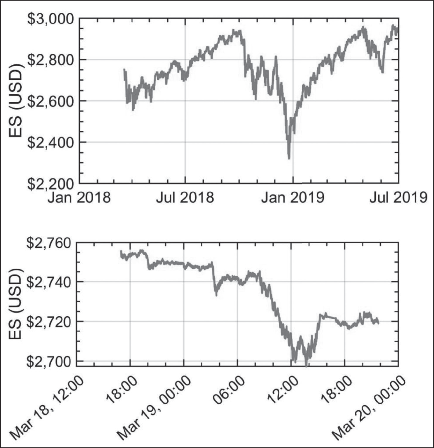
All ES contracts are cash-settled against the value of the underlying S&P 500 equity index at specified annual expiration dates in March, June, September and December. The contract with the nearest expiration date tends to attract most of the trading activity. This is called the ‘front-month’ contract. In this research report, we analyse ‘front-month’ contracts over the period March 2018 through July 2019. During March 18–20, 2018, the front-month contract was the contract expiring in June 2018. During this time, the S&P 500 index fluctuated slightly above 2,700 points, making each E-mini contract worth about $135,000. Each price increment is called the ‘tick’ size; the minimum tick size of ES is 0.25 index points, or $12.50. Therefore, a price move of one tick signifies a fluctuation of about 2.5 basis points. Figure 1 shows the front month E-mini S&P futures time-series used in this study (upper plot), from 3 March 2018 to 28 June 2019. The lower plot shows a small subset of these data.

III. Method of Fractal Analysis

To show that asset prices follow fractal processes is to demonstrate something greater than merely the behaviour of a random walk. Random walks are a specific example of fractality. This implies that fractal processes are a mathematical generalisation of random walks. For situations where signals show fractional Brownian motion (fBm), the signal time-series is to have zero-mean, and it may find expression as the stochastic integral (Mandelbrot & Van Ness, 1968):

B_{H} (t) = \frac{1}{Γ (H + 1 / 2)} \{\int_{- \infty}^{0} [{(t - s)}^{H - 1 / 2} - (- s)^{H - 1 / 2}] d W (s) + \int_{0}^{t} {(t - s)}^{H - 1 / 2} d W (s)\},

where the parameter W is defined as a white noise process over (–∞,∞), and Γ is the well-known gamma function. In the above equation, the parameter H ∈ (0,1), known as the scaling exponent, can also be shown to be related to the Hurst exponent (Peters, 1991). In instances where time-series are relatively smooth, the scaling exponent reaches values near 1. By contrast, when the scaling exponent approaches smaller values nearer 0, the time-series tends towards increasing roughness. All fractal signals, in addition to their roughness also feature self-similarity, and usually it is possible to employ the scaling exponent to directly computer the fractal dimension of the set. Any signal that displays fBm has a covariance function given by

cov \{B_{H} (s), B_{H} (t)\} = \frac{1}{2} {|s |^{2 H} +| t |^{2 H} - | s - t |^{2 H}}

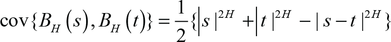
so that the variance $var \{B_{H} (t)\} = t^{2 α}$ , and $B_{H} (0) \equiv 0.$ From this, it is clear that when H=1/2, the situation collapses to the well-known random walk characteristic of the EMH. The FMH results in a generalisation of the EMH to allow other values of the scaling exponent. A time-series is called persistent in situations where scaling exponents are found to be above H=1/2. In such cases, if any point i along the series is selected, and one finds that B(t_i+1)>B(t_i), for example, this means that for the next time-step (i+1) it is more likely than not that the signal will continue with the same sign for its first derivative. That is, the probability is greater than 0.5 that B(t_i+2)>B(t_i+1). On the other hand, when the time-series is found to have a fractal scaling exponent beneath 1/2, then it is call antipersistent. Again, this is because if B(t_i+1)>B(t_i), the probability is greater than 0.5 that the sign of the first derivative will change, that is, B(t_i+2)<B(t_i+1). In a trading context, this means that if the price time-series is persistent, then the current price trend is more likely than not to continue. An antipersistent price series means that any price trend is more likely than not, to reverse, at the next tick.

In physical systems, what is usually found is that fBm is a nonstationary process. What we mean by this is that statistical properties vary throughout the signal. Analysis methods which assume stationarity, therefore, cannot be used. It is thus difficult and requires extreme care to accurately detect the presence of memory in the time-series. Numerous studies have investigated fBm. For instance, in fields as diverse as biology (Collins & De Luca, 1994), hydrology (Neuman & Federico, 2003), geophysics (Frisch, 1997), telecommunication networks (Taqqu et al., 1997), space physics (Consolini et al., 2013; Dobias & Wanliss, 2009) and medicine (Khoa et al., 2012).

Data intermittency is found in both upper and lower plots as shown in Figure 1. In addition, there is long-range dependence, and trends that recur over multiple timescales. It is necessary to have an appropriate method to determine the presence of long-range correlations in the time-series. All of the methods have a general methodology. Usually, they will calculate an estimate of how a fluctuation measure, here denoted by F, scales with the size of the time window considered, denoted by n. Well-known techniques to determine scaling include power spectral analysis, the Higuchi (1988) method, Hurst’s rescaled range analysis (Hurst, 1951), DFA (Peng et al., 1995) and structure function analysis (Abramenko et al., 2002). In every method, all essentially calculate varieties of a fluctuation measure, although the measure is different for each technique.

From our development of previous expertise, we find that DFA has qualities that suit it to analysis of the data here considered (see Figure 1). DFA is a modified root mean squared analysis of a random walk. Peng et al. (1995) improved upon ideas in statistical physics to develop the DFA. It was designed specifically to function with non-linear data, and to be able to deal with data nonstationarity. Numerous studies show that it is one of the most robust statistical techniques designed to detect long-range correlations in time-series (Blok, 2000; Cannon et al., 1997; Taqqu et al., 1996). DFA is thus capable of accurately determining data scaling, and is robust to the presence of trends (Hu et al., 2001) and time-series featuring nonstationarity (Chen et al., 2002; Kantelhardt et al., 2002).

To calculate the data scaling, the DFA analysis technique starts by removing the average, symbolised by $\bar{B}$ , from the time-series, B(t). Next, this series is integrated as follows:

y (k) = \sum_{t = 1}^{k} [B (t) - \bar{B}] .

The investigator next divides this updated time-series into boxes of equal length, n (see Figure 2). Each box has removed from it the trend, represented by a least-squares fit to the data. Usually, the trend function selected a cubic, quadratic or linear function (Hu et al., 2001; Vjushin et al., 2001). For our purposes, we utilise a quadratic function to remove errors due to linear trends in the time-series. Box n has its abscissa denoted by y_n(k). Following this step, the integrated time-series, y(k), is taken and from it trend is removed by subtracting the local trend, y_n(k), within each box.

Now, it is possible to derive the characteristic size of the fluctuations, denoted by F(n), for a given box size n. This is computed from the root mean squared deviation between y(k) and its local trend in each box

F (n) = \sqrt{\frac{1}{N} \sum_{k = 1}^{N} {[y (k) - y_{n} (k)]}^{2}} .

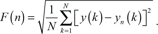
Finally, this calculation is repeated for all the time scales available; these correspond to varying the box size. When a signal is fractal, one finds that relation between F(n) and n follows power-law scaling:

F (n) \propto n^{H},

where the scaling exponent is given by the parameter H. If the time-series is indeed an fBm, then the scaling exponent H, comes out to be the well-known Hurst exponent (Mandelbrot & Van Ness, 1968). For the case, when H = 0.5, the signal is identified as white noise. An antipersistent signal finds H < 0.5, and H > 0.5 reveals a persistent time-series, and strong trends.

IV. Data Properties

As mentioned above, the data we use to explore this hypothesis is the E-mini S&P, designated by the commodity ticker symbol ES. It trades on the CME Globex electronic trading platform. CME Globex trading schedule is Sunday (6:00 p.m.) through Friday (5:00 pm) Eastern Time with a trading halt at 4:15 pm to 4:30 pm on each of the trading days. We consider front month data with open-high-low-close prices from 3 March 2018 to 28 June 2019. The top panel in Figure 1 shows the closing prices for the entire interval, and the bottom panel shows the first 10,000 seconds.

Next, we examine the actual distribution of futures price changes or returns. This is an important issue to financial economists. According to classical statistical theory, a system in an equilibrium state will possess Gaussian statistics for measurable physical quantities. On the contrary, systems that cannot reach an equilibrium state might have probability distributions significantly different from normal ones. This is particularly true for non-linear systems that feature inhomogeneous dissipation in time. In an efficient market, it follows that such equilibrium returns are random. In addition, these random returns are postulated to be normally distributed, which means that asset prices follow log–normal distributions.

As a formal test for normally distributed returns, we consider several parameters that characterise a normal distribution. Determining which data to use in financial analysis is not necessarily clear; Hudson and Gregoriou (2015) found that simple and compound returns can yield significantly different results. Accordingly, we calculated statistics for both simple and compounded returns. Figure 2 shows the simple returns.

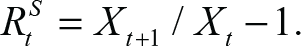
Returns provide the ability to measure investment performance independently of the scale used. We define simple returns in the usual manner, namely, let X be the ES price, at time t. Then, simple return values on the interval [t, t +1] are given by

R_{t}^{S} = X_{t + 1} / X_{t} - 1.

Similarly, compound returns are defined as

R_{t + 1}^{C} = \ln (X_{t + 1}) - ln (X_{t})

Figure 2.

Source: The author.

Table 1.

Results from Several Normality Tests Demonstrate that the Returns for ES Futures Fail the Normal Hypothesis (p-Values are Given for Kolmogorov–Smirnov, Lilliefors and Anderson–Darling Tests)

Test	Simple Returns	Compound Returns
Skewness	–0.51	–0.56
Kurtosis	769	775
Kolmogorov–Smirnov	0.0005	0.0005
Lilliefors	0.001	0.001
Anderson–Darling	0.0005	0.0005

Source: The author.

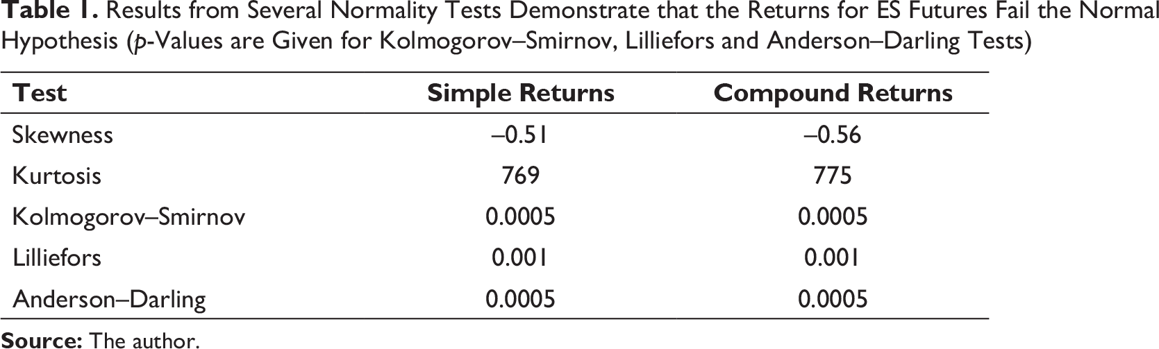
The first normality parameter we consider is skewness. Skewness is a measure of distribution symmetry, and is defined as the normalised third moment of the distribution. A normal distribution has a skewness parameter equalling zero. Skewness is positive (negative) when the data spread out more to the right (left). For our data, the skewness of the simple (compound) returns are, respectively, –0.51(–0.56).

Second, we consider kurtosis, which is a measure of peak steepness of the probability distribution. The normal distribution has kurtosis equal to 3, but heavy-tailed distributions have higher kurtosis. The kurtosis of the simple (compound) returns is, respectively, 769 (775).

Third, we apply the one-sided Kolmogorov–Smirnov test (Marsaglia et al., 2003). We use this non-parametric method to test the null hypothesis that the population cumulative distribution function (cdf) of the data is equal to the normal distribution cdf. The null hypothesis is rejected in favour of the alternative hypothesis, at the default 5 per cent significance level and the p-value is close to zero.

Fourth, we apply the Lilliefors normality test (Conover, 1980; Lilliefors, 1969), which strongly rejects the normality hypothesis, with p ~ 0.

A final test for normality is the Anderson–Darling test (Malevergne & Sornette, 2006) which provides a measure to test the null hypothesis that the data is from a population with a normal distribution. Again, we find, with strong confidence, that the null hypothesis is rejected (p ~ 0). The results of all tests for normality reject the hypothesis that the returns come from a normal distribution, as summarised in Table 1.

V. Data Analysis

Distribution Function

An important question considered in the study of complex systems is what causes the appearance of power law distributions. Suggestions have considered such distributions to be the consequence, and the signature, of self-organising mechanisms at the origin of a hierarchy of scales (Harras & Sornette, 2011; Sornette, 2004, 2009). Given the return distribution functions are significantly different from normal, demonstrated above, the question is what distribution best represents these data. An example of a distribution function P(x) that exhibits the requisite heavy power law probability tail for large x, possibly up to some limiting cut-off, is as follows:

P (x) \propto \frac{C_{μ}}{x^{1 + μ}} .

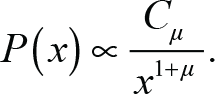
Here, the µ-exponent is a metric characterising the nature of the tail. When µ < 2, the tail is termed a ‘heavy tail’ and has a theoretically undefined variance. Accurate fitting the tails of this kind of an empirical distribution with a power law is notoriously difficult (Bielinskyi et al., 2019; Rachev et al., 2005; Weron, 2001).

Having determined that the ES returns are significantly different from normal, we will compute the empirical ES futures return distribution, and fit it to a stable form, using the method outlined by Koutrouvelis (1980, 1981). We select the stable function for several reasons. First, because the kurtosis in our data is reminiscent of Lévy-stable distributions. Second, heavy-tailed Lévy-type behaviour is common in many physical systems (Wanliss, 2005; Wanliss & Reynolds, 2003), and is finding increasing relevance in economics (Basegmez & Cekici, 2017; Caginalp & Caginalp, 2018; Champagnat et al., 2013). Finally, stable distributions are a very general, broad and rich class of distributions allowing for heavy-tails and skewness. The most common stable distribution is the Gaussian normal curve. Rejecting the assumption of normal distribution of returns supports the hypothesis that a stable distribution is suitable for these data.

A distribution is stable if its shape remains unchanged under sums of the same type. Also, all non-degenerate stable distributions are continuous distributions with infinitely differentiable density. For example, if one took a Gaussian normal distribution, and added a second Gaussian normal distribution to it, the result would remain a Gaussian normal distribution. Every possible stable distribution is a special case of the Lévy alpha-stable distribution, defined by the Fourier transform of its characteristic function (Nolan, 2016),

f (x; α, β, γ, δ) = \int_{- \infty}^{\infty} φ (x) e^{- i t x} d x,

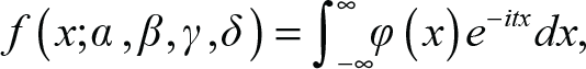
and φ(t) is given by

φ (t) = \exp \{i δ t - γ {|t|}^{α} [1 + i β sign (t) w (t, α)]\},

and

w (t, α) = \{\begin{matrix} t a n \frac{α π}{2}, i f α \neq 1, \\ \frac{2}{π} \log (t), i f α = 1, \end{matrix}

sign (t) = \{\begin{matrix} 1, i f t > 0, \\ 0, i f t = 0, \\ - 1, i f t < 0. \end{matrix}

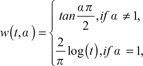
The alpha-stable Lévy distribution function is a function of four variables, α, β, γ and δ. Generally speaking, the α and β statistics are parameters that determine the shape of the distributions. The γ and δ statistics are location parameters.

The first shape parameter, α, is known as the characteristic exponent, or index of stability. It ranges over (0, 2). When α decreases, the central peak gets higher, the regions flanking the peak flatten and the tails at large values get heavier. When α = 2, we recover the Gaussian normal distribution.

The second shape parameter β is the skewness parameter. It ranges over [–1, 1]. This variable determines the thickness, or heaviness, of the tails. When α = 1, β = 0, the Cauchy distribution is obtained, and when α = 0.5, the Lévy distribution is obtained. When β < 0, the distribution skews towards the right tail, when β > 0, the distribution skews towards the left tail. For the case β = 0, the distribution is symmetric, and when β = ± 1, the distribution is completely skewed towards that tail, that is, there is no tail on the other side. An interesting feature of the Gaussian normal distribution (α = 2) is that β has no effect on this distribution.

The meaning of the final two parameters is very simple. The scale is determined by γ; increasing or decreasing the scale will magnify or shrink the distribution. The final variable is the location parameter, δ, which serves to shift the centre of the distribution left or right.

Given the size of the empirical returns for ES, with a mean very close to zero, as seen in Figure 2, it is to be expected that there should be negligible difference between statistical results whether one looks at simple or compound returns. Since the compound return equation yields very small values, the difference between simple and compound returns, at least for the data we examine, is essentially the same, as is shown below, with a Taylor series expansion:

R_{t + 1}^{C} = \ln (X_{t + 1}) - \ln (X_{t}) = \ln (\frac{X_{t + 1}}{X_{t}}) \approx \frac{X_{t + 1}}{X_{t}} - 1 - \frac{1}{2} {(\frac{X_{t + 1}}{X_{t}} - 1)}^{2} + \frac{1}{3} {(\frac{X_{t + 1}}{X_{t}} - 1)}^{3} + \dots \approx \frac{X_{t + 1}}{X_{t}} - 1^{} = R_{t + 1}^{S} .

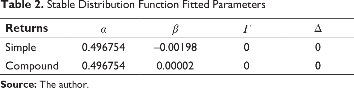
We model the ES returns by calculating the empirical PDF, and using maximum likelihood to estimate the parameters α, β, γ and δ in the alpha-stable distribution. Results for the fit to the empirical PDF of the ES-series are summarised in Figure 3, with parameters given in Table 2. Most of the stable distribution parameters are identical whether from simple or compound returns, except for β, which is slightly, but not significantly, different.

Figure 3.

Source: The author.

Table 2.

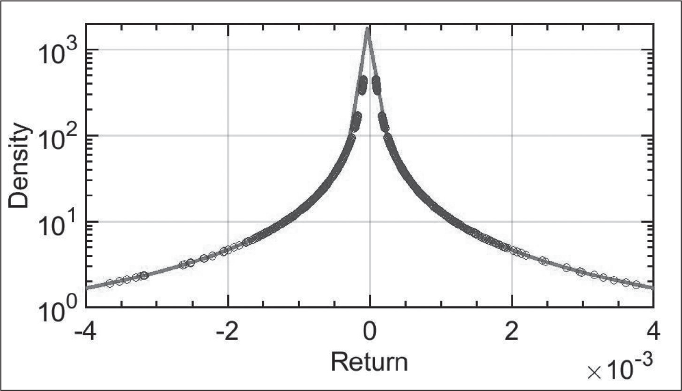
Stable Distribution Function Fitted Parameters

Returns	α	β	Γ	Δ
Simple	0.496754	–0.00198	0	0
Compound	0.496754	0.00002	0	0

Source: The author.

DFA

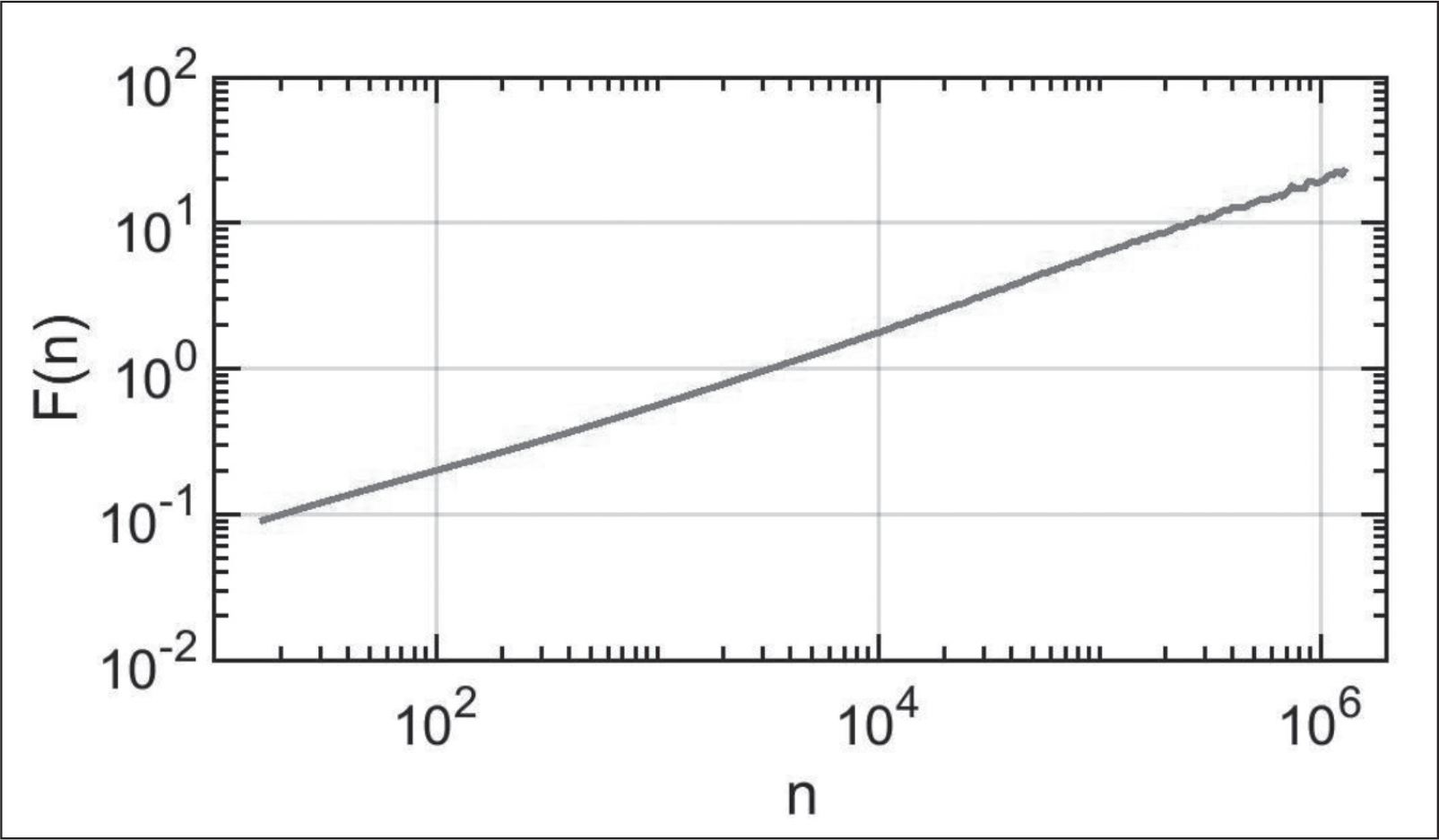
Serlitis et al. (2008) and Uritskaya (2005) demonstrated use of DFA to stock market prices. Here, we perform similar analysis to ES data. Figure 4 shows the DFA of ES prices. The best-fit slope, H, the Hurst exponent, is estimated using non-linear least-squares for a power law. The result for the slope is $H = 0.505 \pm 0.006.$ The scaling exponent purely suggests a random geometric Brownian motion.

VI. Summary and Conclusions

In this article, we have considered whether the E-mini S&P futures market returns follow a random walk, or some other behaviour in its price dynamics. Large, but rare events punctuating periods of relative quiescence are remarkable emergent properties found not only in physical sciences, but also in economics. These events are usually quantified by heavy-tailed distributions of event sizes, in which often unexpected events come to dominate system development. Theoretical considerations suggest that dynamic fluctuations of selling pressure can generate a market crash even in the absence of a fundamental shock (Kirilenko et al., 2017). Huang and Wang (2009) expanded on the theoretical framework of Grossman and Miller (1988), in which an equilibrium model links the cost of maintaining continuous market presence with market crashes even in the absence of fundamental shocks and with perfectly offsetting idiosyncratic shocks. In their model, market crashes emerge endogenously when a sudden excess of sell orders overwhelms the insufficient risk-bearing capacity of market makers.

Figure 4.

Source: The author.

We have found that the ES returns data violate the normality requirement of the EMH, and that returns are fractal. Several tests confirmed the violation of normality. We fitted the ES return distribution to the Lévy alpha-stable process. This process generalises the special case of the normal distribution, and shows how the ES returns have heavy tails, supporting the FMH. Estimates of the four Lévy alpha-stable parameters are consistent with the conjecture that the stochastic process generating the returns is fractal.

We used DFA to determine the Hurst exponent, measuring long-range dependence in ES futures data. This method, from statistical physics, has the advantage that it is better able to deal with nonstationarities than typical methods in financial economics, such as variance analysis. The detrended fluctuation functions were approximately linear over about five decades in log–log space (see Figure 4). Thus, on a long timescale, ES appears monofractal. This suggests that on a scale of approximately 1 year a single scaling controls the dynamics over a wide range of scales. However, it is possible that the scaling exponent varies as a function of time. Since ‘local’ changes in scaling exponents can be observed through DFA, it could be important to consider shorter intervals to get a full view of the non-linear characterisation of ES futures. An improved understanding of the dynamics of these kinds of data are an important part of understanding economic intermittency observed in business cycles and financial markets (Chian, 2007).

The fractal scaling exponent we find is essentially that of a random walk. However, our findings imply that, on the roughly annual scale we have examined, ES financial returns behave in a more general manner than random walks. Random walks are, of course, but a special case of general fractal processes. Technically, this means that deviations from the EMH, and the associated heavy-tailed distributions, are more common than expected. One is thus able to earn (or lose) much more than the Gaussian model predicts. In addition, the analysis reveals that crisis prevention on the basis of the EMH, would be a theoretically flawed methodology with disadvantages compared to the FMH. Our results indicate that the ES futures market operates close to the state predicted by the EMF, but that the observed transient deviations from this state fail to have a statistical origin, consistent with a purely random geometric Brownian motion, and are better described by the FMH. Our results help to improve understanding of dynamical instabilities of ES futures markets and suggest future directions for analysis of multiscale trends within this market.

Footnotes

Declaration of Conflicting Interests

The author declared no potential conflicts of interest with respect to the research, authorship and/or publication of this article.

Funding

The author received no financial support for the research, authorship and/or publication of this article.

References

Abramenko

V. I.

Yurchyshyn

V. B.

Wang

Spirock

T. J.

Goode

P. R.

(2002). Scaling behaviour of structure functions of the longitudinal magnetic field in active regions on the sun. Astrophysical Journal , 577, 487.

Abreu

Brunnermeier

M. K.

(2003). Bubbles and crashes. Econometrica , 71(1), 173–204.

Bak

(1997). How nature works: The science of self-organized criticality . Oxford University Press.

Basegmez

Cekici

(2017). Financial applications of stable distributions: Implications on Turkish stock market. Journal of Business Economics and Finance , 6(4), 364–374. Retrieved from https://doi.org/10.17261/Pressacademia.2017.769.

Bielinskyi

Semerikov

Solovieva

Soloviev

(2019). Levy’s stable distribution for stock crash detecting. Paper presented at the SHS Web of Conferences, 65, 06006. Retrieved from https://doi.org/10.1051/shsconf/20196506006.

Bil

Ł.

Grech

Zienowicz

(2017). Asymmetry of price returns—Analysis and perspectives from a non-extensive statistical physics point of view. PLoS One , 12(11), e0188541. Retrieved from https://doi.org/10.1371/journal.pone.0188541.

Black

Scholes

(1973). The pricing of options and corporate liabilities. Journal of Political Economy , 81(3), 637–654. doi:10.1086/260062.

Blok

H. J.

(2000). On the nature of the stock market: Simulations and experiments (PhD thesis). University of British Columbia, Canada.

Bouchaud

J.-P.

Potters

(2003). Theory of financial risks: From statistical physics to risk management , 2nd ed. Cambridge University Press.

10.

Caginalp

(2018). The quotient of normal random variables and application to asset price fat tails. Physica A: Statistical Mechanics Applications , 499, 457–471.

11.

Cannon

M. J.

Percival

D. B.

Caccia

D. C.

Raymond

G. M.

Bassingthwaighte

J. B.

(1997). Evaluating the scaled windowed variance methods for estimating the Hurst coefficient of time series. Physica A: Statistical Mechanics Applications , 241, 606.

12.

Champagnat

Deaconu

Lejay

Navet

Boukherouaa

(2013). An empirical analysis of heavy-tails behavior of financial data: The case for power laws . HAL archives-ouvertes.

13.

Chen

Ivanov

P. Ch.

Stanley

H. E.

(2002). Effect of nonstationarities on detrended fluctuation analysis. Physical Review E: Statistical, Nonlinear Soft Matter Physics , 65, 041107.

14.

Chian

A. C.-L

. (2007). Complex systems approach to economic dynamics . Springer.

15.

Collins

J. J.

De Luca

C. J.

(1994). Upright, correlated random walks: A statistical-biomechanics approach to human postural control system. Chaos , 5(1), 57.

16.

Conover

W. J.

(1980). Practical nonparametric statistics . Wiley.

17.

Consolini

De Marco

De Michelis

(2013). Intermittency and multifractional Brownian character of geomagnetic time series. Nonlinear Processes Geophysics, 20, 455–466. doi:10.5194/npg-20-455-2013.

18.

Corazza

Malliaris

A. G.

Nardelli

(1997). Searching for fractal structure in agricultural futures markets. Journal of Futures Markets , 17(4), 433–473.

19.

Dobias

Wanliss

J. A.

(2009). Intermittency of storms and substorms: Is it related to the critical behaviour. Annales Geophysicae , 27, 2011–2018. doi:10.5194/angeo-27-2011-2009.

20.

Dorigo

Di Caro

Sampels

(2002). Ant algorithms . Springer.

21.

Derman

Taleb

N. N.

(2005). The illusions of dynamic replication. Quantitative Finance , 5(4), 323–326.

22.

Fama

E. F.

(1970). Efficient capital markets: A review of theory and empirical work. Journal of Finance , 25, 383–417.

23.

Fama

E. F.

(1991). Efficient capital markets II. Journal of Finance , 46, 1575–1617.

24.

Frisch

(1997). Turbulence . Cambridge University Press.

25.

Grossman

Miller

(1988). Liquidity and market structure. Journal of Finance , 43, 617–633.

26.

Harras

Sornette

(2011). How to grow a bubble: A model of myopic adapting agents. Journal of Economic Behavior & Organization , 80, 137–152. doi:10.1016/j.jebo.2011.03.003.

27.

Higuchi

(1988). Approach to an irregular time series on the basis of the fractal theory. Physica D: Nonlinear Phenomena , 31, 277–283.

28.

Ivanov

P. Ch.

Chen

Carpena

Stanley

H. E.

(2001). Effect of trends on detrended fluctuation analysis. Physical Review E: Statistical, Nonlinear Soft Matter Physics , 64, 011114.

29.

Huang

Wang

(2009). Liquidity and market crashes. Review of Financial Studies , 22, 2607–2643.

30.

Hudson

R. S.

Gregoriou

(2015). Calculating and comparing security returns is harder than you think: A comparison between logarithmic and simple returns. International Review of Financial Analysis , 38, 151–162. Retrieved from https://doi.org/10.1016/j.irfa.2014.10.008.

31.

Hurst

H. E.

(1951). The long term storage capacity of reservoirs. Transactions American Society Civil Engineers , 116, 770–799.

32.

Kantelhardt

J. W.

Zschiegner

S. A.

Koscielny-Bunde

Havlin

Bunde

Stanley

H. E.

(2002). Multifractal detrended fluctuation analysis of nonstationary time series. Physica A: Statistical Mechanics Applications , 316, 87–114.

33.

Khoa

T. Q.

V. Q.

Toi

V. V.

(2012). Higuchi fractal properties of onset epilepsy electroencephalogram. Computational and mathematical methods in medicine, 2012, 461426. doi:10.1155/2012/461426.

34.

Kirilenko

Kyle

A. S.

Samadi

Tuzun

(2017). The flash crash: High‐frequency trading in an electronic market. Journal of Finance , 72, 967–998. doi:10.1111/jofi.12498.

35.

Koutrouvelis

I. A.

(1980). Regression-type estimation of the paramters of stable laws. Journal American Statistical Association , 75(372), 918–928.

36.

Koutrouvelis

I. A.

(1981). An iterative procedure for the estimation of the parameters of stable laws. Communications Statistics–Simulation Computation, 10(1), 17–28.

37.

Kurov

Lasser

(2004) Price dynamics in the regular and E-mini futures market. Journal of Financial and Quantitative Analysis , 39, 365–384.

38.

Lilliefors

H. W.

(1969). On the Kolmogorov-Smirnov test for the exponential distribution with mean unknown. Journal American Statistics Association , 64, 387–389.

39.

Longin

F. M.

(2016). Extreme events in finance: A handbook of extreme value theory and its applications . Wiley.

40.

Malevergne

Sornette

(2006). Extreme financial risks (Vol. 16). Springer.

41.

Mandelbrot

B. B.

Van Ness

J. W.

(1968). Fractional Brownian motions, fractional noises and applications. SIAM Review , 10, 422–437.

42.

Mantegna

R. N.

Stanley

H. E.

(2000). An introduction to Econophysics: Correlations and complexity in finance. Cambridge University Press.

43.

Marsaglia

Tsang

Wang

(2003). Evaluating Kolmogorov’s distribution. Journal of Statistical Software , 8(18).

44.

Mitsutake

Otsuka

Oinuma

Ferguson

Cornelissen

Wanliss

Halberg

(2004). Does exposure to an artificial ULF magnetic field affect blood pressure, heart rate variability, and mood. Biomedicine & Pharmacotherapy , 58(Suppl. 1), S20–S27. https://doi.org/10.1016/S0753-3322(04)80004-0.

45.

Neuman

S. P.

Federico

V. D.

(2003). Multifaceted nature of hydrogeologic scaling and its interpretation. Reviews Geophysics , 41(3). doi:10.1029./2003RG000130.

46.

Nolan

J. P.

(2016). Stable distributions: Models for heavy tailed data . Springer.

47.

Peng

C.-K.

Havlin

Stanley

H. E.

Goldberger

A. L.

(1995). Quantification of scaling exponents and crossover phenomena in nonstationary heartbeat timeseries. Chaos , 5(1), 82.

48.

Peters

E. E.

(1991). A chaotic attractor for the S&P 500. Financial Analyst Journal , 47(2), 55–62.

49.

Peters

E. E.

(1994). Fractal market analysis . Wiley.

50.

Qian

X.-Y.

G.-F.

Zhou

W.-X.

(2011). Modified detrended fluctuation analysis based on empirical mode decomposition for the characterization of anti-persistent processes. Physica A: Statistical Mechanics Applications , 390 (23–24), 4388–4395. doi:10.1016/j.physa.2011.07.008.

51.

Rachev

S. T.

Stoyanov

S. V.

Biglova

Fabozzi

F. J.

(2005). An empirical examination of daily stock return distributions for U.S. stocks. In Baier

Decker

Schmidt-Thieme

(Eds.), Data analysis and decision support: Studies in classification, data analysis, and knowledge organization . Springer.

52.

Samuelson

(1965). Proof that properly anticipated prices fluctuate randomly. Industrial Management Review , 6, 41–49.

53.

Serlitis

Uritskaya

O. Y.

Uritsky

V. M.

(2008). Detrended fluctuation analysis of the US stock market. International Journal of Bifurcation and Chaos , 18(2), 599–603. Retrieved from https://doi.org/10.1142/S0218127408020525.

54.

Sornette

(2004). Critical phenomena in natural sciences: Chaos, fractals, self-organization and disorder: Concepts and tools, 2nd edn., Springer Series in Synergetics . Springer.

55.

Sornette

(2009). Probability distributions in complex systems, Core article for the encyclopedia of complexity and system science. Editor-in-chief: R. A. Meyers , 10370, p. 4300 illus. Springer. Vols. 11, ISBN: 978-0-387-75888-6 (arxiv.org/abs/0707.2194).

56.

Taqqu

M. S.

Teverovsky

Willinger

(1996). Estimators for long-range dependence: An empirical study. Fractals , 3, 785–798.

57.

Taqqu

Teverovsky

Willinger

(1997). Is network traffic self-similar or multifractal. Fractals , 5, 63–73.

58.

Trichet

J.-C.

(2010). What can central banks do in a financial crisis? Speech by Mr Jean-Claude Trichet, President of the European Central Bank, on the occasion of the Susan Bies Lecture, Kellogg Distinguished Lecture Series, Evanston, Illinois, 27 April 2010, 1–12.

59.

Uritskaya

(2005). Forecasting of magnitude and duration of currency crises based on the analysis of distortions of fractal scaling in exchange rate fluctuations. In Abbott

Bouchaud

J.-P.

Gabaix

McCauley

J. L.

(Eds.), Noise and fluctuations in econophysics and finance, Proceedings of SPIE , Vol . 5848. SPIE. doi:10.1117/12.609400.

60.

Vandewalle

Ausloos

(1997). Coherent and random sequences in financial fluctuations. Physica A: Statistical Mechanics Applications , 246, 454–459.

61.

Vjushin

Govindan

R. B.

Monetti

R. A.

Havlin

&Bunde

(2001). Scaling analysis of trends using DFA. Physica A: Statistical Mechanics Applications , 302, 234–243.

62.

Wanliss

J. A.

Reynolds

M. A.

(2003). Measurement of the stochasticity of low-latitude geomagnetic temporal variations. Annales Geophysicae , 21, 2025–2030.

63.

Wanliss

J. A.

(2004). Nonlinear variability of SYM-H over two solar cycles. Earth Planets Space , 56, e13–e16.

64.

Wanliss

J. A.

(2005). Fractal properties of SYM-H during quiet and active times. Journal Geophysical Research , 110, A03202. doi:10.1029/2004JA010544.

65.

Weron

(2001). Levy-stable distributions revisited: Tail index > 2 does not exclude the Levy-stable regime. International Journal of Modern Physics C , 12, 209–223.

66.

Working

(1934). A random-difference series for use in the analysis for time series. Journal of the American Statistical Association , 29, 11–24.

67.

Zhou

W.-X.

(2007). A guide to econophysics . Shanghai University of Finance and Economics Press.