Fiscal Discipline and Its Relationship with Economic Growth in India: Evidence-based Policy Analysis

Abstract

This study attempts to make an empirical analysis to evaluate the procedural progress of India in terms of public policy parameters. The study constructs a composite Fiscal Performance Index (FPI) for the period 1990–2018. The reported values show that the FPI has been significantly increasing over the last two-three decades. However, it is clearly evident that the fiscal discipline was slightly poor during the period 1998–1999 to 2003–2004. Since 2003–2004, there has been a consistent increasing trend in the fiscal discipline till 2007–2008 global financial crisis. The constructed index was further utilised to establish its relation with economic growth. The causal relationship from FPI to GDP growth is evident in the long run. The study suggests that, as a federal nation, the Central government should encourage governments at all levels to promote fiscal discipline by formulating macroeconomic policies in line with the Fiscal Responsibility and Budget Management Act, 2003.

Keywords

Economic growth fiscal policy fiscal sustainability Fiscal Responsibility and Budget Management (FRBM) Act 2003

Introduction

The present study attempts to create a composite index of fiscal discipline for India for two reasons. First, policymakers are constantly in the process of designing effective policies to achieve the set goals. It is necessary to design policies by targeting the root cause of the problem, keeping a vision of its consequences. The precondition for shaping such productive public policy, in the economic sense, is to be well-equipped with the fiscal situation of the economy (Arai, 2011; Daniel & Goa, 2015; Glomm & Kumar, 1996; Hagen & Harden, 1996). An index comprising fiscal dimensions better indicates the overall status of the fiscal condition of an economy. With the help of such an index, policymakers can design optimum public policies that can further influence the size of the economy.

Second, in the aftermath of the global financial crisis (2008), many governments and Central banks worldwide responded to it; Government of India also tried to deal with this crisis by spending more money than its revenue. As a result, the fiscal deficit had considerably widened (Narayan, 2018; Srinivas, 2018). At the same time, the lack of adequate growth in the supply of goods and services led to demand-pull inflation (Kumar & Soumya, 2010; Narayan, 2018). A higher fiscal deficit was eventually spilt into the external sector, resulting in widening the current-account deficit and depreciating the nominal value of the Rupee in the foreign exchange market. Thus, the weak Rupee prevented foreign portfolio investment and slowed the inflow of forex reserves. Since then, fiscal discipline has been seen as a focal point of most discussion at the Central level. As a result, the accountability of the government has gained momentum in managing funds, with profitability of public expenditure, and the utilisation of revenue generated. Over the past couple of decades, several attempts have been made to evaluate the fiscal performance of India (Confederation of Indian Industry (CII), 2019; Government of India, 2000, 2005; Jangili et al., 2022; Mohanty & Mishra, 2016).

Eleventh Finance Commission (EFC) took steps in addressing the issue of measuring the fiscal discipline. The terms of reference of EFC state that restructuring of public finances of states and Centre to restore the budgetary balance and maintain macroeconomic stability is an objective. EFC adopted a single-indicator-based method to evaluate fiscal policy discipline, namely, Fiscal Self-Reliance and Improvement Index (FSRII). This FSRII was given a 7.5% weight in the distribution formula. The Twelfth Finance Commission also recommended this single-indicator index for measuring fiscal discipline and gave it equal weight tax collection effort. However, the problem with the single-indicator index is that it does not cover all the dimensions of the government’s fiscal behaviour. In addition, an inaccurate weightage distribution between given measure leads to an incomplete assessment of fiscal policy discipline. It is also believed that the summary index of fiscal policy discipline should reveal how the fiscal imbalance is sought to be corrected (Sucharita & Sethi, 2011). In this context, while correcting the errors highlighted above, the present study aims at creating a broad index fiscal policy discipline, taking into account six broad indicators for the period 1990–2018. Subsequently, using this index, the present study also empirically examines the relationship between fiscal policy discipline and the size of economic activity in India.

The rest of the study is structured as follows. While the second section covers the relevant literature review on constructing fiscal performance index (FPI), the third section discusses the data and methods adopted in the study. The fourth section discusses the study’s empirical results, and the last section concludes the study by providing suggestions for policymakers.

Literature Review

This section provides a brief literature review on two aspects: fiscal discipline and economic growth. The first group of studies (Bhide & Panda, 2002; Dash, 2011; Dholakia, 2005; Emes, 1999; Mohanty & Mishra, 2016) solely focused on assessing fiscal policy discipline using multiple indicators approach. Emes (1999), for instance, considers three dimensions while constructing a composite index of fiscal performance of the Canadian provinces and the US states. These dimensions reflect changes in spending in government revenues and taxation structures. This index consists of two sub-indices made up of fourteen variables. The first sub-index examines as to what extent the governments have controlled spending during their terms of office and is composed of ten variables. The second sub-index examines how taxes and revenues have changed over the same period and is composed of four variables. Similarly, Dholakia (2005) suggests a multi-dimensional, more stable index to evaluate the progress of Indian states in terms of various fiscal parameters. The author considers eight fiscal indicators, reflecting different aspects of fiscal performance and combines them into three broad indices—Deficit Index, Own-Revenue Effort Index, and Expenditure and Debt Repayment Index, which are connected to form a composite FPI. The study justifies using a multiple-indicator approach rather than a single-indicator approach to measure the fiscal discipline of the Indian states. Dash (2011) tries to evaluate whether the fiscal performance of a Special-Category State—Tripura, is improved after implementing the fiscal reforms during 1990–1991 to 2008–2009. The index for Tripura consists of three individual indices, namely, Deficit Indicator Index, Own Revenue Effort Index, and Expenditure-and Debt-Serving Index. Each of these indicators consists of eight key fiscal ratios. The study concludes that the fiscal management of the Tripura State over the study period is progressively improved, and the year 2007–2008 is identified as the best fiscal performance year. Similarly, using Relative Distance and Z-score methods, Mohanty and Mishra (2016) analyse the fiscal performance of seventeen non-special category states for the period 2003–2004 to 2014–2015. The study constructs a composite FPI, which comprises five major sub-indices, and each of these sub-indexes consists of two minor sub-indices. The study indicates a decline in FPI level over the mentioned period and huge inter-state variations in the level of FPI.

On the other hand, the second group of studies (Fatás & Mihov, 2008; Kamila, 2021; Misra & Trivedi, 2015) entirely focused on exploring the impact of such composite policy discipline indices on economic growth. These studies essentially seek to emphasise the role of fiscal management in economic growth. The empirical evidence of these studies ultimately confirms that fiscal discipline has a positive-growth effect. However, in some cases, the evidence is incomplete and silent concerning the causal direction between fiscal discipline and economic growth. Similarly, many other scholars have studied the impact of policy changes on output growth from an empirical perspective. Alesina et al. (1996) study the effects of political instability on growth; the papers provide evidence in favour of the hypothesis that political instability impairs growth. Fatás (2002) also provides evidence that the relationship between volatility and growth is negative and significant for poor countries, but negligible and non-significant for high-income countries. A recent study on the effects of fiscal discipline on output growth by Evans (2020) shows that policy uncertainty; corruption and fiscal deficits have a significant negative relationship with economic development and economic growth in both the short and long terms. The study further evidences that budgetary reforms have a significant positive relationship with economic growth in the long run.

Data and Methods

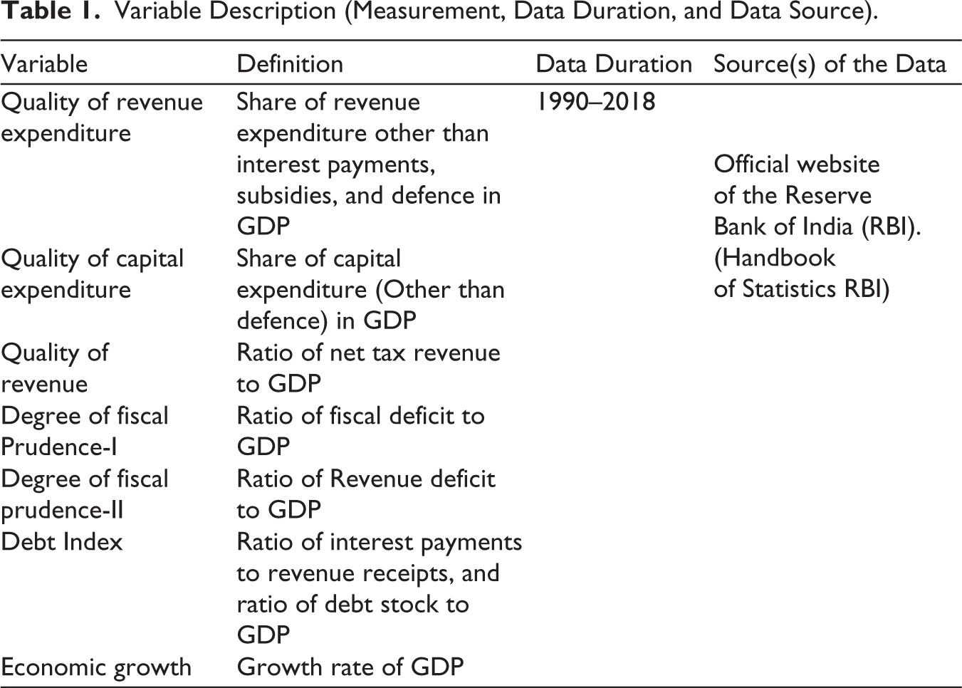
This study has used time-series annual data, which have been collected from the official website of the Reserve Bank of India (RBI). The period of the study is 1990–2018. Principal Component Analysis is used to construct the FPI. The Auto-Regressive Distributed Lag Model (ARDL) co-integration method has been employed to demonstrate the relationship between the constructed index and economic growth. As reported in Table 1, this study takes seven indicators to estimate six components reflecting various facets of fiscal performance. The six major proxies are taken into account to construct FPI for India, which include, Quality of Revenue Expenditure measured by the share of revenue expenditure other than interest payments, subsidies, and defence in GDP, Quality of Capital Expenditure measured by the share of capital expenditure (other than defence) in GDP, Quality of Revenue has calculated the ratio of net tax revenue to GDP. Degree of Fiscal Prudence-I is depicted as a fiscal deficit to GDP, and Degree of Fiscal Prudence-II is portrayed as revenue deficit to GDP. Finally, proxy in this regard is Debt Index developed, using two minor sub-indices such as interest payment to revenue receipt index (IPRRI) and outstanding debt ratio index (DRI). Interest payment to revenue receipt index is computed by the ratio of interest payments to revenue receipts, indicating the percentage of revenue receipts used for interest payment on account of outstanding debt. It represents the debt-servicing position of the country. Similarly, DRI is constructed as the ratio of debt stock to GDP (DS/GDP). This index reflects the debt burden of the country. The debt index is formed by the arithmetic mean of the IPRRI and DRI.

Table 1.

Variable Description (Measurement, Data Duration, and Data Source).

Variable	Definition	Data Duration	Source(s) of the Data
Quality of revenue expenditure	Share of revenue expenditure other than interest payments, subsidies, and defence in GDP	1990–2018	Official website of the Reserve Bank of India (RBI). (Handbook of Statistics RBI)
Quality of capital expenditure	Share of capital expenditure (Other than defence) in GDP
Quality of revenue	Ratio of net tax revenue to GDP
Degree of fiscal Prudence-I	Ratio of fiscal deficit to GDP
Degree of fiscal prudence-II	Ratio of Revenue deficit to GDP
Debt Index	Ratio of interest payments to revenue receipts, and ratio of debt stock to GDP
Economic growth	Growth rate of GDP

Each indicator is first normalised to the scale of 0–100, where zero is the worst value, and 100 is the best value by using the relative distance method. It can take both favourable and adverse parameters to construct an index. The index which is constructed for a favourable indicator is called the Improvement Index. The index which is formed by taking adverse parameters is called the Deprivation Index.

Deprivation Index (D) = \frac{Max (X) - X)}{Max (X) - Min (X)} \times 100

Improvement Index (I) = \frac{Y - Min (Y)}{Max (Y) - Min (Y)} \times 100

where X refers to the actual value of the parameter for a given state, Max (X) and Min (X) are the maximum and minimum value of the particular parameter across the states in a specified period, and Y can be interpreted like X with the condition X≠Y.

The first three components are treated as Improvement Index as favourable indicators. The last three components are treated as Deprivation Index. In case of the Improvement Index, a higher ratio gives a high index value, while the Deprivation Index is constructed in such a way that the lower the ratio for a year, a higher index value shall be assigned to it. The other issue in constructing an index is the choice of weights for each of the component variables. The issue is not just to give the appropriate weight to each of the component statistics but to also take into account any correlation between the component statistics. The principal components method of factor analysis determines the weights for the various components using statistical methods that exploit the correlation between observations. Furthermore, it reduces the information in many variables to the smaller set of factors and determines the actual elements in the set, which are required to explain the maximum variance.

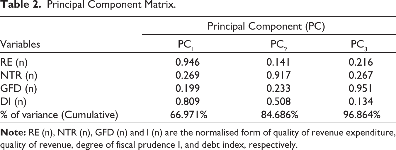
This method keeps on extracting the variables until the variance explained by an additional extracted factor would be less than the explanation of anyone of the individual variables. The extracted factors are orthogonal to each other, so they do not share any information. The weights of the components are given by the rotated component matrix. These weights are then multiplied by the selected principal components reported in Table 2. Finally, the FPI is constructed by taking the weighted mean for each year.

Table 2.

Principal Component Matrix.

Variables	Principal Component (PC)
Variables	PC₁	PC₂	PC₃
RE (n)	0.946	0.141	0.216
NTR (n)	0.269	0.917	0.267
GFD (n)	0.199	0.233	0.951
DI (n)	0.809	0.508	0.134
% of variance (Cumulative)	66.971%	84.686%	96.864%

Note: RE (n), NTR (n), GFD (n) and I (n) are the normalised form of quality of revenue expenditure, quality of revenue, degree of fiscal prudence I, and debt index, respectively.

The growth rate of GDP is used as the proxy for economic growth, and the constructed FPI is used to depict the fiscal performance of India. The linear regression analysis has been employed to check if there exists any short-run causal relationship between these two variables. Before doing the regression analysis, it is required to check if the data are stationary or not. If data are not stationary, then using the Ordinary Least Square (OLS) method tends to generate spurious regression results. To avoid this, the augmented Dickey–Fuller test has been conducted. Further, the empirical analysis is carried ahead using the following simple regression equation

GDP = c + b (FPI)

Similarly, a long-run co-integration test has been employed to further evaluate any long-term relationship between these variables. Given the time-series properties of the variable considered in the study, ARDL model is employed to examine the long-run relationship between economic growth and FPI for India during 1990–2018.

Results and Discussion

Before applying Principal Components Analysis, we tested for suitability of data using Bartlett’s test of sphericity and Kaiser–Meyer–Olkin (KMO) measure of sampling adequacy. For KMO, a value of above 0.6 confirmed the factorability and Bartlett’s test of sphericity revealed statistical significance at the 1% level. The first two components – Quality of Capital Expenditure and Degree of Fiscal Prudence II—are removed from the analysis as they could not fulfil the measure of sampling adequacy.

Since first three principal components (PC1) cumulatively capture 96.8% of the total variance, the top four values (0.946, 0.917, 0.951, and 0.809) for the given four proxies from these three components have been used for constructing the final index.

The individual index for each year is calculated by multiplying the normalised value of the component by their respective weights. Finally, the FPI for each year is constructed by adding all the calculated indexes of four variables for the respective year, presented in Figure 1.

Figure 1.

Fiscal Discipline Trend in India Over 1991–2018.

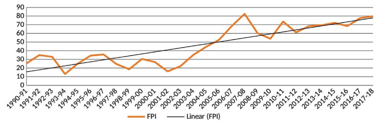
The results show that the FPI has been significantly increasing over the last two-three decades. However, it is clearly evident from Figure 1 that fiscal discipline was slightly poor during the period 1998–1999 to 2003–2004. Since 2003–2004, there has been a consistent increasing trend in the fiscal discipline till 2007–2008 global financial crises. It might be due to the implementation of Fiscal Responsibility and Budget Management (FRBM) Act, 2003.

Unfortunately, the FRBM targets were suspended due to the global financial crisis. As the Global Financial Crisis led to a sudden collapse of domestic and international demands, the inflow of foreign capital into the country slowed and eventually led to the collapse of economic growth. As a result, the Union government had to postpone its fiscal goals and inflate resources into the economy with a variety of economic stimuli. Consequently, the country’s gross fiscal deficit widened to 6% of GDP in 2008–2009 and 6.4% in 2009–2010. Similarly, the revenue deficit increased from 1.1% to 4.5% of GDP in 2008–2009 and 5.2% in 2009–2010. Thus the goals set by FRBM Act, 2003, due to the global financial crisis, were significantly violated. Therefore, the value of the FPI fell from 82.46 in 2007–2008 to 53.81 in 2009–2010.

However, the Union Finance Minister, Pranab Mukherjee, in his 2011–2012 Budget speech announced that amendments to the FRBM Act would be introduced through the 2012 Finance Bill. This Finance Bill proposed a new target for the reduction of fiscal and revenue deficits. Accordingly, the FRBM Act was amended in May 2013 as a result of these proposals. The term ‘effective revenue deficit’ was also introduced in the FRBM Act by the 2012 Finance Bill. Thus, attempts were made to put fiscal discipline in the groove. The result has been a steady increase in the value of FPI since then. These findings corroborate the analysis of the CII.

The augmented Dickey–Fullertest has been conducted to determine whether the series is stationary. Although it is found that FPI is of integrated order 1, GDP growth is found to be stationary at levels. A new series is formulated, which is the first difference of FPI, denoted as D (FPI). This was carried out to avoid spurious regression results. The short-run analysis regression equations using OLS are

GDP = (1) + (2) \times D (FPI)

and

FPI = (1) + C (2) \times GDP

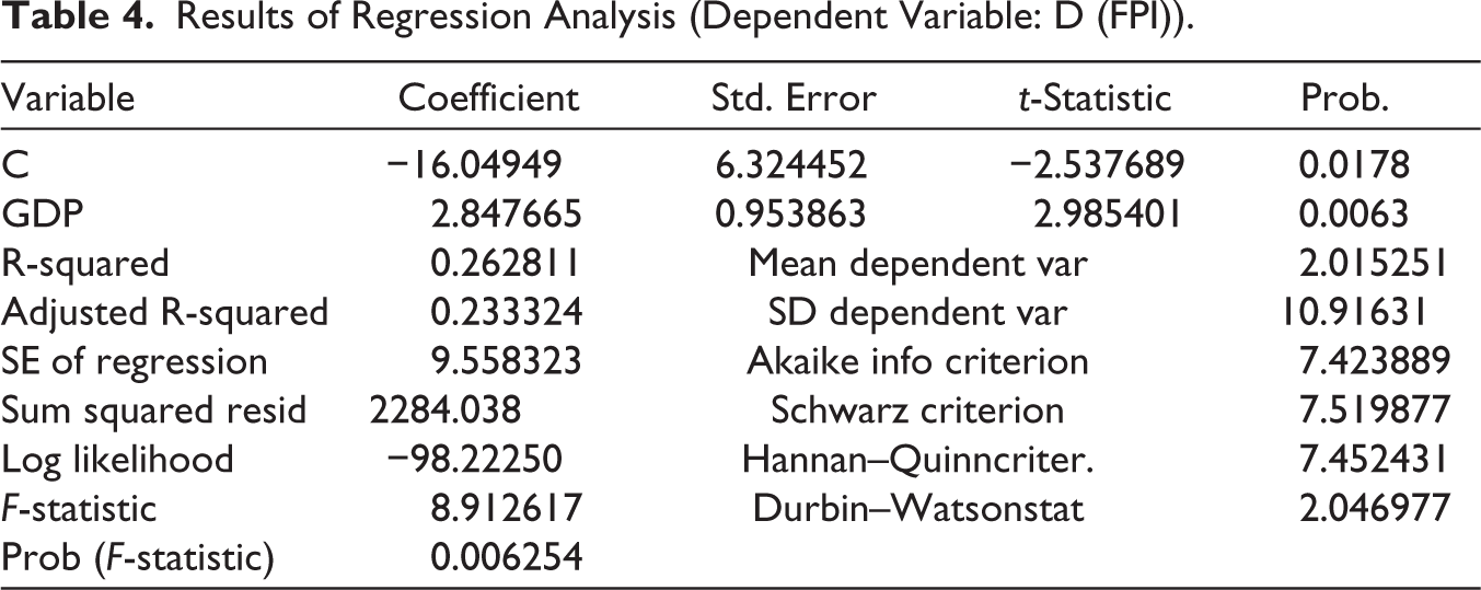
It is found in Tables 3 and 4 that there seems to be a short-term causal relationship between FPI to GDP and GDP to FPI. The value of R-squared for both the regression analysis is 0.26. It implies a two-way causal relationship between these two in the short run.

Table 3.

Results of Regression Analysis (Dependent Variable: GDP Growth Rate).

Variable	Coefficient	Std. Error	t-Statistic	Prob.
C	6.157716	0.336965	18.27403	0.0000
D(FPI)	0.092290	0.030914	2.985401	0.0063
R-squared	0.262811	Mean dependent var		6.343704
Adjusted R-squared	0.233324	SD dependent var		1.965209
SE of regression	1.720738	Akaike info criterion		3.994571
Sum squared resid	74.02350	Schwarz criterion		4.090559
Log likelihood	−51.92671	Hannan–Quinncriter		4.023113
F-statistic	8.912617	Durbin–Watsonstat		1.377088
Prob (F-statistic)	0.006254

Table 4.

Results of Regression Analysis (Dependent Variable: D (FPI)).

Variable	Coefficient	Std. Error	t-Statistic	Prob.
C	−16.04949	6.324452	−2.537689	0.0178
GDP	2.847665	0.953863	2.985401	0.0063
R-squared	0.262811	Mean dependent var		2.015251
Adjusted R-squared	0.233324	SD dependent var		10.91631
SE of regression	9.558323	Akaike info criterion		7.423889
Sum squared resid	2284.038	Schwarz criterion		7.519877
Log likelihood	−98.22250	Hannan–Quinncriter.		7.452431
F-statistic	8.912617	Durbin–Watsonstat		2.046977
Prob (F-statistic)	0.006254

In the long run, both Granger and Johansen’s methods do not fit this data with variables of different integrated order (1) and I (0). As suggested in various literatures available in such cases, an ARDL structure is used, and a Bound test is conducted to verify if there is any long-run relationship. The equation for ARDL is

GDP = C (1) \times GDP (- 1) + C (2) \times FPI + C (3) \times FPI (- 1) + (4)

As discussed above, this study is based on the t-Bounds test. The null hypothesis is given as there is no level relationship, and the Bounds test is conducted twice, changing the dependent variable. First, the dependent variable is the GDP growth rate, and the calculated t-statistic value is more than the value of I (1) bound at a 5% level of significance. The results are such that the null hypothesis cannot be rejected. It implies a long-run relationship between the two, and FPI is causing the GDP growth rate.

Similarly, the same is done by keeping FPI as a dependent variable. The results reported in Table 5 show the calculated t-statistic value is less than the I (0) bounds at a 5% significance level. The results are such that the study fails to reject the null hypothesis. It implies that the GDP growth rate is not causing the FPI in the long run.

The co-integration equation obtained by the Bounds test is

\begin{array}{l} GDP = 4.98 - 1.03 \times GDP (- 1) + 0.031 \times \\ (GDP - (0.03 \times F (- 1)) + 0.11 \times D (FPI)) \end{array}

Table 5.

t-Bounds Test Results (Dependent Variable: GDP Growth Rate).

Test Statistic	Value	Null-Hypothesis: No Levels Relationship
Test Statistic	Value	Significance	I(0)	I(1)
t-statistic	−5.432896	10%	−2.57	−2.91
		5%	−2.86	−3.22
		2.5%	−3.13	−3.5
		1%	−3.43	−3.82

The empirical results of long-run causality reported in Table 6 prove a long-run causal effect from FPI to GDP growth rate.

Table 6.

t-Bounds Test (Dependent Variable: FPI).

Test Statistic	Value	Null-Hypothesis: No levels Relationship
Test Statistic	Value	Significance	I(0)	I(1)
t-statistic	−1.755497	10%	−2.57	−2.91
		5%	−2.86	−3.22
		2.5%	−3.13	−3.5
		1%	−3.43	−3.82

Concluding Remarks

This study attempts to measure India’s composite FPI for a period from 1990–1991 to 2017–2018. The FPI is constructed by taking six components derived from seven indicators. It is observed that the FPI has been significantly increasing over the last two decades. However, it is found that fiscal discipline was slightly poor during the period 1998–1999 to 2003–2004. Since 2003–2004, there has been a consistently increasing trend in the fiscal discipline till the global financial crisis (2007–2008). The constructed index was then further utilised to establish a relation with economic growth using the Autoregressive Distributed LagCo-integration technique. The study also found that there is a two-way causal relationship between fiscal discipline proxied by FPI and GDP growth. But in the long run, the causal relationship from FPI to GDP growth is evident. Thus, it is apparent that the policies targeting a strong FPI will positively impact India’s economic growth in the long run.

This study contains some essential policy suggestions for the country. Since irresponsible fiscal management, corruption and policy uncertainties are the leading causes of unsustainable economic policies and thus to economic instability in India, governments at all levels should make significant efforts to implement concrete reforms that promote fiscal discipline and transparency in public spending. Efforts in these directions can contribute to better economic development. In addition, as a federal nation, the Central government should encourage governments at all levels of the country to promote fiscal discipline and facilitate further development by formulating macroeconomic policies in line with the FRMB Act, 2003. Radical reforms on inter-governmental transfers in India must be brought about to promote inter-state fiscal discipline, and the Finance Commission must consolidate all revenue transfers between them. Such reforms, generally, are of paramount importance in promoting economic growth and reducing the fiscal deficit ratio to a sustainable value in the long run. The present study proves that fiscal discipline leads to economic growth in India. However, the lack of information may question the validity of the evidence provided by only 17 samples. Therefore, it is believed that a future effort can be made by extending the time series data on India to see how the causal pattern between fiscal discipline and economic growth in India evolves over time.

Footnotes

Declaration of Conflicting Interests

The authors declared no potential conflicts of interest with respect to the research, authorship and/or publication of this article.

Funding

The authors received no financial support for the research, authorship and/or publication of this article.

Appendix

References

Alesina

, Sule

, Nouriel

, & Phillip

(1996). Political instability and economic growth. Journal of Economic Growth, 1, 189–211.

Arai

(2011). Productive government expenditure and fiscal sustainability. Public Finance Analysis, 67(4), 327–351.

Bhide

, & Panda

(2002). Evaluating quality of budgets with a composite index. Economic & Political Weekly, 37(13), 1177–1180.

Confederation of Indian Industry (CII). (2019, June 7). Measuring fiscal marksmanship: Is fiscal deficit the only measure? Confederation of Indian Industry. https://cii.in/PublicationDetail.aspx?enc=vhrFxd7VqiQU3OeYraljnmcZRqVJYB7dzpbioq9h+Uk=

Daniel

B. C.

, & Goa

(2015). Implications of productive government spending for fiscal policy. Journal of Economics and Dynamics and Control, 55, 148–175.

Dash

A. K.

(2011). Fiscal performance of special category states in India: A case study of Tripura state finance. Euro Economica, 3(27), 121–132.

Dholakia

(2005). Measuring fiscal performance of states: an alternative approach. Economic & Political Weekly, 31(30), 3421–3428.

Emes

(1999). Fraser Institute fiscal performance index (Occasional Paper No. 20). Fraser Institute, Public Policy Sources.

Evans

(2020). Fiscal discipline, financial development & economic growth in Nigeria. In Nwaogwugwu

C. I.

(Ed.), Dynamics of fiscal and monetary policies in ECOWAS countries. University of Lagos Press.

10.

Fatás

(2002). The effects of business cycles on growth. In Loayza

& Soto

(Eds.), Economic growth: Sources, trends and cycles (pp. 191–216). Central Bank of Chile.

11.

Fatás

, & Mihov

(2008). Fiscal discipline, volatility and growth. In Perry

(Ed.), Prudence or abstinence: Fiscal policy, stabilization, and growth. World Bank. https://www.ecotec.edu.ec/material/material_2017X1_ECO520_01_96612.pdf

12.

Glomm

& Kumar

R. B.

(1996). Productive government expenditures and long-run growth. Journal of Economic Dynamics and Control, 21(1), 183–204.

13.

Government of India. (2000, June). Report of the eleventh finance commission. https://fincomindia.nic.in/writereaddata/html_en_files/oldcommission_html/fcreport/eleventhrep.htm

14.

Government of India. (2002, December). Report of the twelfth finance commission. https://fincomindia.nic.in/writereaddata/html_en_files/oldcommission_html/fcreport/Report_of_12th_Finance_Commission/12fcreng.pdf

15.

Government of India. (2005, June). Report of the eleventh finance commission. https://fincomindia.nic.in/TFC/13fcreng.pdf

16.

Hagen

J. V.

, & Harden

(1996). Budget process and commitment to fiscal discipline [Working Paper No. WP/96/78]. International Monetary fund (IMF). http://www.adbi.org/working-paper/2010/09/17/4075.fiscal.policy.issues.india.after.gfc/

17.

Jangili

, Kumar

N. R. V. V. M. K. R.

, & Chander

(2022). States’ fiscal performance and yield spreads on market borrowings in India [Working Paper Series No.04]. RBI. https://www.rbi.org.in/Scripts/PublicationsView.aspx?id=20995

18.

Kamila

(2021, November 24). Fiscal dominance in India: an empirical estimation [Working Paper No. 359]. NIPFP. https://www.nipfp.org.in/media/medialibrary/2021/11/WP_359_2021.pdf

19.

Kumar

, & Soumya

(2010, September). Fiscal policy issues for India after the global financial crisis (2008–2010) [Working Paper No. 249]. Asian Development Bank Institute.

20.

Misra

, & Trivedi

(2015). Structural fiscal balance: an empirical investigation for India (Occasional Paper No 35 & 36 (1&2)). RBI. https://rbidocs.rbi.org.in/rdocs/Content/PDFs/4SFIBAL388EAC1FB8E64A87BCC7780BF2950DA9.PDF

21.

Mohanty

A. R.

, & Mishra

B. R.

(2016). Fiscal performance index of the states in India. Prajnan, 55(3), 247–267.

22.

Narayan

(2018, September 11). Global financial crisis: Lessons for India from the 2008 crisis and beyond. Business Standard.

23.

Srinivas

(2018, September 14). 10 years after global financial crisis, India’s fiscal deficit still not back to pre-crisis levels. Hindustan Times.

24.

Sucharita

& Sethi

(2011). Fiscal discipline in India. Romanian Journal of Fiscal Policy, 2(1), 1–23.