
Abstract
That the long-term unemployed fare worse in the labor market than do the short-term unemployed is well-known, but why? One potential explanation is that the long-term unemployed are “bad apples” who had poorer prospects from the outset of their spells (heterogeneity). Another is that these bad outcomes are a consequence of their extended unemployment (state dependence). The authors use Current Population Survey data on unemployed individuals linked to unemployment insurance wage records for the same people to distinguish between these explanations. The rich work history information contained in the wage records allows the authors to control for individual heterogeneity that could affect post-unemployment labor market outcomes. Even with these controls in place, they find that unemployment duration has a strongly negative effect on the likelihood of subsequent employment. The results are robust to accounting for differences in the labor market conditions experienced by the long-term and short-term unemployed.
Keywords
Long-term unemployment soared during and in the immediate aftermath of the Great Recession of 2007 to 2009. Even as the economy recovered in the following years, long-term unemployment remained stubbornly high. The number of people unemployed for 27 weeks or more rose from 1.1 million at the start of 2007 to a peak of 6.8 million in April 2010 and did not fall below 5 million until September 2012. The long-term share of total unemployment exceeded 40.0% from December 2009 through November 2012 and remained elevated compared to its pre-recession level eight years after the recession’s trough. This article provides new evidence on how experiencing a spell of long-term unemployment affects subsequent employment and earnings.
Concern that the long-term unemployed might have become permanently detached from the labor market rose in the wake of the Great Recession and the dramatic increase in long-term unemployment that followed. In an analysis using Current Population Survey (CPS) data, Krueger, Cramer, and Cho (hereafter KCC) (2014) found that, among those who had been unemployed 27 weeks or more as first-wave CPS respondents during 2008 to 2012, only 35.9% were employed 15 months later and just 10.8% were in full-time jobs that had lasted at least four months. While those who had been unemployed for a shorter period (26 weeks or less) also appear to have experienced significant labor market challenges—in the same data, only 49.5% of the short-term unemployed were employed 15 months later and just 14.4% were in full-time stable jobs—outcomes for the long-term unemployed were notably poorer. These findings are robust to controlling for observable worker characteristics such as age, gender, and education.
The finding that the long-term unemployed have fared less well than the short-term unemployed during the recent recovery period echoes earlier findings in the literature on the evolution of the job-finding hazard. Kaitz (1970) first documented that longer unemployment durations are associated with lower exit rates and others have found this to be true specifically for exits from unemployment to employment. It is less clear why the long-term unemployed experience poorer job-finding prospects than those who are more recently unemployed. One set of explanations rests on possible sources of state-dependence. Long-term unemployment may have a causal effect on the job-finding rate because of human capital depreciation during spells away from work (Mincer and Ofek 1982; Acemoglu 1995; Stratton 1995; Albrecht, Edin, Sundstrom, and Vroman 1999; Gorlich and de Grip 2009), decreases in search intensity over the spell of unemployment (Krueger and Mueller 2011; Faberman and Kudlyak 2014), or employer discrimination against the long-term unemployed in hiring (Ghayad 2013; Kroft, Lange, and Notowidigdo 2013; Eriksson and Rooth 2014, but see Farber, Silverman, and von Wachter 2017). Alternatively, what appears as a decline in the job-finding rate could instead be the result of heterogeneity among the unemployed such that, at longer durations, more of the unemployed are “bad apples” with personal attributes that lead to their having poorer job-finding prospects (Cripps and Tarling 1974; Heckman and Singer 1984). The interpretation of the findings of KCC (2014) depends critically on whether the outcomes for the long-term unemployed are a result of the time they have spent in that state (i.e., are causal) or reflect underlying unobserved heterogeneity.
In data consisting of information on a single spell of unemployment for each included sample member, it is challenging to fully distinguish between these competing explanations. After reviewing a number of studies that have attempted this task, Machin and Manning (1999) concluded that “it does not really seem possible in practice to identify separately the effect of heterogeneity from that of duration dependence without making some very strong assumptions about functional form which have no foundation in any economic theory” (p. 3111).
One possible approach to distinguishing between the contributions of state dependence versus underlying heterogeneity as explanations for the decline in the job-finding hazard at longer unemployment durations is to exploit the information contained in multiple spells of unemployment for the same individuals, as in Alvarez, Borovickova, and Shimer (2015). In this article, we have adopted a different but related approach. Borrowing from methods used in the job displacement literature, we use information on individuals’ employment experiences prior to their becoming unemployed to control for heterogeneity in employment propensities as well as heterogeneity in the trajectory of those employment propensities that might explain subsequent employment outcomes. To the extent that the long-term unemployed are less likely to become employed even after controlling in this way for underlying heterogeneity, we can feel more confident about attaching a causal interpretation to the relationship between unemployment duration and job-finding success.
Related to the question of how longer versus shorter spells of unemployment affect subsequent employment is the question of how they affect subsequent earnings. On the one hand, setting a higher reservation wage and searching longer for a better match could lead to higher earnings on the jobs eventually accepted by the long-term unemployed (Ehrenberg and Oaxaca 1976; Acemoglu and Shimer 2000). On the other hand, evidence suggests that unemployed individuals turn down relatively few job offers based on wages (Schmieder, von Wachter, and Bender 2016). To the extent that job searchers target their best opportunities first, this might lead one to expect a negative association between unemployment duration and subsequent earnings. Heterogeneity among the unemployed such that those with lower labor market productivity also take longer on average to find a job could produce the same pattern. We address the impact of differing durations of unemployment on subsequent earnings using essentially the same methods as just described for studying impacts on subsequent employment.
In addition to the literature on the consequences of experiencing unemployment for subsequent labor market outcomes, our article is closely related to the literature on job displacement. The central question in this literature concerns the adverse impact of job displacement on subsequent labor market outcomes, especially subsequent earnings. In addressing this question, we take into account both the prior level and the prior trajectory of earnings. Our formal analysis borrows heavily from the approach taken in the job displacement literature (e.g., Farber 1993, 1997, 2005, 2013, 2015; Jacobson, LaLonde, and Sullivan 1993; Couch and Placzek 2010; Davis and von Wachter 2011; von Wachter, Song, and Manchester 2011). One difference between the population of displaced workers—typically, long-tenure workers who have lost their jobs during a mass layoff—and the population of unemployed individuals we study is that the unemployed include not only job losers but also new entrants to the labor market, labor market re-entrants, and people who voluntarily left their previous job.
To carry out our analysis, we have created a matched employer–employee data set based on individuals who responded to the CPS from 2003 through 2010 that combines information on individuals’ labor force status and personal characteristics from the CPS with information on their employment and earnings histories from unemployment insurance (UI) wage records. Similar to KCC (2014) and consistent with other evidence on job-finding rates by duration of unemployment, we find that CPS respondents with longer unemployment durations are less likely than the short-term unemployed to be employed in subsequent quarters. To illustrate, in a model that controls for observable demographic characteristics such as age, gender, and education as well as year, individuals unemployed five quarters (53–65 weeks) at the time of their CPS interview are 14.6 percentage points less likely to have UI jobs eight quarters later than those unemployed for one quarter (1–13 weeks) as of the CPS interview date.
This pattern could be driven by unobserved differences in underlying employment propensities between the long-term and the short-term unemployed. In a balanced panel, it is possible to compare the employment rate in a period that follows a spell of unemployment to the pre-unemployment employment rate for the same set of people. In our empirical implementation, we compare the employment rate eight quarters after a group is observed in the CPS to the employment rate for the same group eight quarters earlier. The magnitude of any change in the employment rate for the long-term unemployed can then be contrasted with that for the short-term unemployed. The advantage of this approach is that it removes the effects of fixed unobservable factors on employment rates from the comparison of outcomes across the unemployment duration groups. Adopting this approach tends to raise, not lower, the estimated adverse impact of being long-term unemployed rather than short-term unemployed on subsequent employment—for example, the 14.6 percentage point estimate of the relative disadvantage associated with having been unemployed for five quarters rather than one quarter cited in the previous paragraph increases to 19.8 percentage points. This outcome is because, except for those reporting unemployment of six quarters or more, the longer-term unemployed were actually more likely to have been employed eight quarters prior to being observed in the CPS than those in the shortest-duration unemployment group.
By contrast, accounting for the effects of different underlying employment trajectories reduces our estimates of the relative disadvantage experienced by the long-term unemployed. This finding is mainly because a disproportionate share of the short-term unemployed are young adults, and employment rates for that age group are generally rising over time. Constructing a post-unemployment benchmark for employment that takes into account the differences in employment trajectories across the unemployment duration groups thus makes the post-unemployment outcomes of the short-term unemployed look relatively worse. Our preferred estimates, after allowing for fixed individual differences in employment propensities and for differences in employment trajectories related to both observable and unobservable individual characteristics, imply that those unemployed five quarters (53–65 weeks) at the time of their CPS interview experienced employment losses that are 13.5 percentage points greater than the losses experienced by those unemployed just one quarter (1–13 weeks), not very different from the 14.6 percentage point estimate obtained by simply comparing post-unemployment outcomes across the same unemployment duration groups.
These findings suggest that extended unemployment leads to negative labor market consequences, but an alternative explanation might be that the long-term unemployed have experienced more adverse shocks or weaker external labor market conditions, and this is why they are less likely to obtain subsequent employment. Two pieces of evidence suggest that this cannot be the whole story. First, we observe very similar patterns with regard to the relative disadvantage of the long-term unemployed in obtaining subsequent employment when we narrow our focus to those who entered unemployment due to having lost a job. Second, controlling in our regression models for the rate of employment growth in an individual’s state, or in the individual’s state and industry, has almost no effect on the estimated relationship between unemployment duration and subsequent employment rates.
An additional question on which we are able to provide new evidence is how experiencing a longer versus a shorter spell of unemployment affects an individual’s subsequent earnings. Average earnings for a group of unemployed individuals in any later period depend both on the probability that members of the group become employed and on the amount earned by those who are employed. In an analysis of average earnings that mimics the analysis of the relationship between unemployment duration and employment just summarized, we obtain very similar results. Our preferred estimates imply that the long-term unemployed experience earnings losses that are much larger than those for the short-term unemployed. This finding is attributable mainly to differences in the probability of having a job as opposed to differences in earnings conditional on having a job.
Data
The data used in our analysis consist of CPS records matched to Longitudinal Employer-Household Dynamics (LEHD) micro-data for the same individuals. The CPS collects information on labor force activity and demographics from the members of approximately 60,000 households per month. The LEHD is a longitudinally linked employer–employee data set created at the U.S. Census Bureau. The LEHD rests on administrative records from states’ unemployment insurance (UI) systems that contain information on the earnings of all covered workers in that quarter, often referred to as wage records, along with Quarterly Census of Employment and Wages (QCEW) data that contain information about the establishments at which these workers are employed. Every quarter, employers who are subject to state UI laws—approximately 98% of all private-sector employers, plus state and local governments—are required to submit information on their workers (the wage records) and their workplaces (the QCEW) to the state UI agencies. The wage records and the QCEW data provided to the Census Bureau by the state agencies are combined and enhanced with various census and survey micro-data to create the LEHD. Abowd et al. (2009) provided a thorough description of the source data and the methodology underlying the LEHD data.
For recent years, the LEHD comes close to being a universe of all workers with wage and salary employment in the US private sector, state government, or local government. Because states have joined the LEHD at different points in time, however, data for fewer states are available in earlier years. Data for 31 states, which account for approximately 70% of the US population, are available beginning in 1998, and our main analysis uses LEHD data for these 31 states. 1
The CPS identifier needed to link the CPS and LEHD records—the Protected Identification Key or PIK—is available for all March CPS respondents. Our sample consists of respondents to the 2003 through 2010 March CPSs who lived in one of the 31 states for which LEHD data are available from 1998 onward and for whom we have a PIK. The LEHD records are the source of the prior and future employment histories used in our analysis. The linked data set incorporates LEHD data for the period from 1998 through 2012, meaning that we can follow all of the unemployed individuals in our sample backward in time for at least 20 quarters and forward in time for at least 11 quarters from the date of their CPS interview (provided they remain in the states for which we have LEHD data). In addition, the LEHD includes information on earnings for each reported job, so that we are able to observe the prior and future earnings profiles of the CPS respondents.
Our interest lies primarily with those who are classified as unemployed in the CPS as of the date of the CPS-LEHD match. For comparison purposes, we also construct similar employment and earnings profiles for those the CPS classifies as employed and for those the CPS classifies as not in the labor force (NILF). One complication is that the PIK is missing for about 20 to 30% of CPS respondents. We use propensity score methods similar to those described in Abraham, Haltiwanger, Sandusky, and Spletzer (2013) to re-weight the observations for those for whom we have a PIK so that they represent the entire population. 2 A small number of people report being unemployed in two successive March CPSs. We have not attempted to exploit this feature of the data, instead treating person-year observations in the CPS as independent.
Weighted tabulations of the linked CPS observations in our 31-state sample closely match published national tabulations. Online Appendix Figure A.1 presents the 2003 to 2010 time series of the CPS employment-to-population ratio and the unemployment rate from our weighted data (labeled as AHSS in the figure) and from the BLS website (labeled as BLS in the figure). The BLS data are non-seasonally adjusted statistics for the month of March. The AHSS line tracks the BLS line almost perfectly. Online Appendix Figure A.2 presents similar graphs for the percentage of unemployed in each of several unemployment duration categories (< 5 weeks, 5–10 weeks, 11–14 weeks, 15–26 weeks, 27–51 weeks, and ≥ 52 weeks). Again, the weighted AHSS time series are essentially identical to the published estimates.
In our 31-state data set, we do not observe UI jobs reported by employers in the other 19 states or the District of Columbia. If, for example, the long-term unemployed were more likely than the short-term unemployed to move to a non-covered state to take a job, this could be a source of bias in our estimates. By 2005, the coverage of the LEHD had expanded to 48 states accounting for approximately 96% of the US population. To assess whether our findings might have looked different had the coverage of the LEHD data used in our main analysis been broader, we have carried out a sensitivity analysis using LEHD data for the 48 states available in later years. In this sensitivity analysis, we use records for the people living in our 31-state sample who responded to the March CPS in 2008, 2009, or 2010. In that shorter time period, the results are little affected by whether we use UI job information based on the 31-state sample or on the larger 48-state sample. 3 This outcome suggests that we do not need to be concerned about possible biases in our main analysis resulting from the long-duration unemployed having different cross-state mobility propensities than the short-duration unemployed.
Table 1 presents descriptive statistics of the outcome variables and many of the explanatory variables used in our analysis. We are interested in how subsequent labor market outcomes differ for people who have been unemployed for longer versus shorter lengths of time as of the date of the CPS-LEHD link. Descriptive statistics are reported separately for people who had been unemployed up to 13 weeks, 14–26 weeks, 27–39 weeks, 40–52 weeks, 53–65 weeks, or more than 65 weeks as of the March CPS reference week, referred to as the one, two, three, four, five, and six-plus quarter unemployment duration groups. For comparison, descriptive statistics for people who reported in the CPS that they were employed at the time of the CPS-LEHD link also are reported. The numbers of underlying observations in each of these groups is shown at the bottom of the table.
Weighted Sample Characteristics
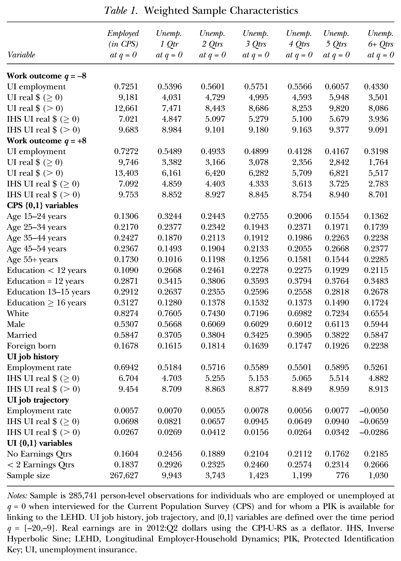
Notes: Sample is 285,741 person-level observations for individuals who are employed or unemployed at q = 0 when interviewed for the Current Population Survey (CPS) and for whom a PIK is available for linking to the LEHD. UI job history, job trajectory, and {0,1} variables are defined over the time period q = [–20,–9]. Real earnings are in 2012:Q2 dollars using the CPI-U-RS as a deflator. IHS, Inverse Hyperbolic Sine; LEHD, Longitudinal Employer-Household Dynamics; PIK, Protected Identification Key; UI, unemployment insurance.
The first two panels of Table 1 report employment and earnings variables based on the UI wage records contained in the LEHD for the periods of eight quarters prior to and eight quarters following the CPS-LEHD link quarter. People who are employed in the CPS at q = 0 (the link quarter) have a 72 to 73% UI employment rate both two years before and two years after the link quarter. Conditional on having UI employment, the CPS employed have average real quarterly earnings of $12,661 two years before and $13,403 two years after the link quarter. The pre-unemployment employment rates and average earnings for persons who are unemployed at q = 0 are much lower than those for the employed, and this is even more true of their post-unemployment employment rates and earnings. In the q = −8 quarter, those who later become longer-term unemployed generally have somewhat higher employment rates and earnings than those who later become short-term unemployed. In the q = +8 quarter, the pattern of differences across the unemployment duration groups is reversed.
The table also reports values of the Inverse Hyperbolic Sine (IHS) of earnings as of q = −8 and q = +8. The IHS of a variable x is defined as:

For x > 0 and especially for x far from zero, this expression is approximately equal to ln(x) shifted by a constant (the ln of 2). Unlike the ln(x) transformation, however, the IHS transformation can be applied to zero values, with IHS(0)=0. Quarters with zero earnings are common in our data and, for that reason, we have adopted the IHS transformation of earnings for our analysis. 4
The next few rows of Table 1 display information regarding the demographic characteristics of each of the groups, as measured in the CPS as of q = 0. These include age, education, race, gender, marital status, and nativity. The differences in age across the unemployment duration groups are especially notable. The proportion of people age 15 to 24 is much higher, and the proportion of people age 45-plus is much lower, in the shorter unemployment duration groups than in the longer unemployment duration groups.
Table 1 also reports average values for a set of variables intended to characterize individuals’ job histories over the 12-quarter period q = {–20,–9}. These variables include the percentage of the 12 quarters for which UI employment is recorded, average IHS(UI earnings) over the 12 quarters and, for the set of people for whom it can be calculated, average IHS(UI earnings) over the quarters with positive UI earnings. Consistent with the differences observed eight quarters prior to the CPS-LEHD link quarter, employment rates and earnings are consistently higher over the q = {–20,–9} period for those who are employed in the CPS at q = 0 than for those who are unemployed. The differences across unemployment duration groups are more modest, though there is some suggestion of stronger prior labor market attachment among those with longer unemployment durations as compared to those in the one-quarter unemployment duration group.
In addition, Table 1 displays estimates of the mean trajectories in employment rates and IHS(earnings) over the q = {–20,–9} period. These trajectories are estimated as the coefficient on a time trend variable in an individual-specific regression fit using the relevant set of observations—all 12 quarters for the employment rate and unconditional IHS(earnings) trajectories and quarters with positive earnings for the conditional-on-working IHS(earnings) trajectory. Estimation of the unconditional earnings trajectory requires at least one quarter of positive earnings and estimation of the conditional earnings trajectory requires at least two quarters of positive earnings; these trajectories are set to 0 in cases for which they cannot be estimated. The indicator variable “No Earnings Qtrs” takes the value of 1 for those with no UI earnings in any quarter over the q = {–20,–9} period; the indicator variable “< 2 Earnings Qtrs” takes the value of 1 for those with no or just one quarter of UI earnings over the same period. There is little to indicate a systematic relationship between the estimated trajectories and how long a person has been unemployed, but those in the short-duration unemployment group are notably more likely not to have worked at all over the q = {–20,–9} period than those in any of the longer unemployment duration groups. 5
Employment and Earnings Profiles
A simple way to glean some initial insights into the labor market consequences of longer versus shorter spells of unemployment is to use our data to plot employment probabilities and measures of earnings for the time periods before and after the CPS-LEHD link quarter. Many of the conclusions to be drawn from the more formal analysis that follows can be previewed in these employment and earnings profiles.
Employment Profiles for the Full Matched Sample
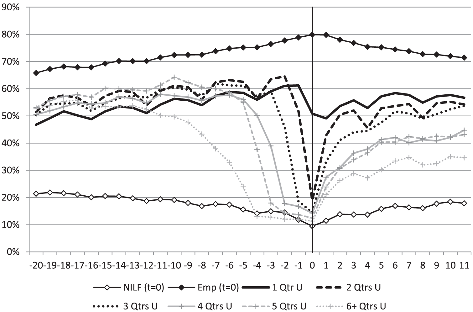
Figure 1 displays employment profiles based on our linked data for employed, NILF, and unemployed individuals. The horizontal axis in the figure is time period, normalized so that q = 0 is the quarter of the CPS-LEHD match (i.e., the quarter including the March in which the individual’s labor force status is recorded in the CPS). Data for 2003 through 2010 have been pooled, so that q = 0 represents different calendar years for different people; in our more formal regression analyses, we estimate models that include year dummy controls. The points to the left of q = 0 along the horizontal axis are the 20 quarters preceding the quarter of the CPS-LEHD link q = {–20,…,–1} and those to the right are the 11 quarters following the quarter of the CPS-LEHD link q = {1,…,11}. The vertical axis in the figure is the weighted percentage of individuals with UI employment in the indicated quarter.
Employment Probabilities
The solid line with black diamonds at the top of the figure shows the quarter-by-quarter UI employment probabilities for people who reported in the CPS that they were employed during the q = 0 March survey reference week. Of those reporting CPS employment in March, 79.9% had at least one UI job during the first quarter of that same year. One reason this statistic is not 100% is that the UI data do not capture federal government employment or self-employment, meaning that someone with CPS employment of those types might not be recorded as employed in the UI data. In addition, from our previous research (Abraham et al. 2013), we know that a significant share of CPS respondents report CPS wage and salary employment in UI-covered sectors during the first quarter of the year but have no corresponding UI wage records in that quarter. The 79.9% UI employment rate for those classified as employed in the March CPS thus is generally in line with our priors. 6 Reflecting the fact that people may move into and out of employment, the UI employment probabilities for the q = 0 CPS employed resemble a shallow inverted V across time. Even in quarters other than q = 0, however, the UI employment rates for the group classified as CPS employed at q = 0 consistently exceed 65%.
The solid line with white diamonds at the bottom of Figure 1 shows the UI employment probabilities for people who report being NILF in the March CPS. Among those in this group, 9.5% have a UI-covered job at some point during the first quarter of the same year. We would not expect this percentage to be zero, since individuals who are working in January or February but not in March should be included here. Looking either backward or forward in time, the percentages of those NILF in q = 0 who have UI employment rise. Those who are NILF at q = 0 but employed in prior quarters will include some older people who have recently retired; those who are NILF at q = 0 but subsequently employed will include some younger people who are just entering the labor force. Because their experience is not obviously relevant for the questions in which we are interested, we have not incorporated the NILF in our subsequent analysis.
The most important information presented in Figure 1 is the pattern of UI employment probabilities for those who are classified as unemployed in the CPS. Separate employment probability profiles are shown for those who had been unemployed up to 13 weeks (which we term the one quarter unemployed), 14–26 weeks (two quarter unemployed), 27–39 weeks (three quarter unemployed), 40–52 weeks (four quarter unemployed), 53–65 weeks (five quarter unemployed), or more than 65 weeks (six-plus quarter unemployed) as of the March CPS reference week.
One initially surprising feature of these plots is the 10 to 20% employment rate in the q = 0 quarter among those who are classified in the March CPS as having been unemployed 14 or more weeks. Similar employment rates also are observed for prior quarters that, based on the duration of unemployment reported in the CPS, began after the start of the individual’s current unemployment spell (e.g., the 18.6% employment rate in q = −1 for those in the three-quarter unemployment group whose unemployment spells are reported to have started 27 or more weeks previously). A literal interpretation of what it means to be unemployed implies that almost no one in our sample should have done any work for pay during quarters that began after the start of their unemployment spell. 7 Previous research has found, however, that reported unemployment durations do not always correspond strictly to the unemployment concept (see, for example, Clark and Summers 1979). Individuals who move from employment to unemployment or from out of the labor force to unemployment in the CPS commonly report initial unemployment durations of more than the 4 or 5 weeks elapsing between survey reference periods (Elsby, Hobijn, Şahin, and Valletta 2011; Kroft, Lange, Notowidigdo, and Katz 2016). The sizable UI employment rates during the time span of reported unemployment may simply indicate that the employment in question is not considered by the respondent to be a “real” job. Consistent with this interpretation, the earnings on jobs held during the q = 0 quarter by individuals classified as unemployed in the CPS are substantially lower than the earnings on jobs held prior to the start of the same individuals’ unemployment spells. Accepting that some UI employment will be reported even during quarters in which work is not expected, the employment probabilities to the left of q = 0 seem very consistent with the unemployment durations recorded in the CPS, in the sense that, for each duration group, the number of quarters in the period prior to the CPS interview with a UI employment rate of less than 20% aligns precisely with the quarters of unemployment the group reports.
The economic questions motivating our article relate to the subsequent labor market trajectories of those observed as unemployed in the CPS. Figure 1 makes clear that, consistent with the findings of KCC (2014), those with shorter unemployment spells are substantially more likely to be employed two to three years after their unemployment spell is recorded in the CPS than those with longer reported unemployment spells. Focusing on the period 8 to 11 quarters following the CPS link quarter, individuals with up to one quarter of unemployment (1–13 weeks) at q = 0 have an average employment rate of 56.6%, those with up to two quarters of unemployment (14–26 weeks) a 53.4% employment rate, those with up to three quarters of unemployment (27–39 weeks) a 51.4% employment rate, and those with up to four or five quarters of unemployment (40–52 or 53–65 weeks) a 42.3% employment rate. The transition from unemployment to eventual employment also appears to occur somewhat more quickly for the short-term unemployed than for the long-term unemployed.
We are especially interested in the extent to which the substantial differences in post-spell outcomes across unemployment duration groups are driven by the differences in unemployment spell length (representing a causal effect) as opposed to being a result of heterogeneity across groups that pre-dated the start of the unemployment spell. Our approach to controlling for unobserved heterogeneity is to compare post-spell employment probabilities to pre-spell employment probabilities within duration groups. Figure 1 shows that 55 to 60% of individuals with one to five quarters of unemployment at q = 0 were employed eight quarters earlier, before their spell of unemployment began. Further, for each of these unemployment duration groups, the probability of being employed was relatively steady with a slight upward drift over the several years before the start of the unemployment spell. Some of those with six or more quarters of unemployment could already have been unemployed even as far back as two years before the link quarter, but their employment rates three years before q = 0 are very similar to those of the other unemployment duration groups. In what follows, we focus mainly on the first five unemployment duration groups. The similarity in pre-spell employment rates across these duration groups stands in sharp contrast to their distinctly different post-spell rates. This finding is prima facie evidence that the outcomes for those in the different unemployment duration groups are not simply a reflection of pre-existing heterogeneity in their employment propensities.
Earnings Profiles
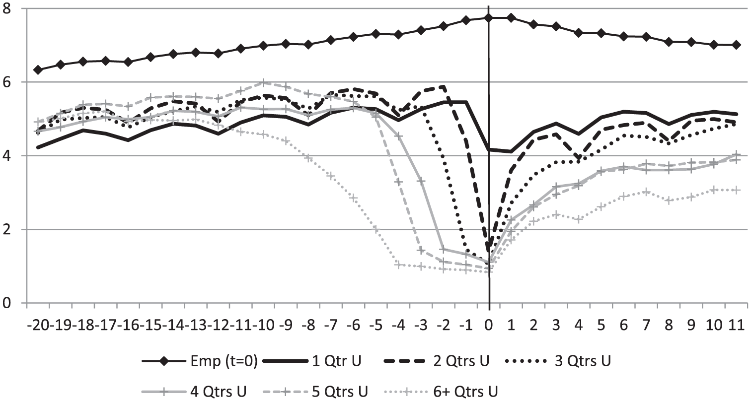
In addition to learning about the pre-unemployment and post-unemployment employment profiles associated with short-term and long-term unemployment, we are interested in the corresponding earnings profiles. We look separately at the path of UI earnings both overall (including people with zero earnings) and among those who succeed in finding a job (and thus have positive earnings). For groups defined on the basis of having CPS employment or belonging to one of the six unemployment duration groups as of the CPS link quarter, Figure 2 plots the mean of the IHS of real UI earnings. Figure 2A includes everyone in our matched sample even if they had no earnings in a given quarter; Figure 2B includes only those people who have positive earnings in a given quarter, and thus speaks more directly to the magnitude of the earnings losses of the long-term unemployed relative to the short-term unemployed with respect to the earnings they eventually accept.
Real Earnings (IHS Earnings ≥ 0)
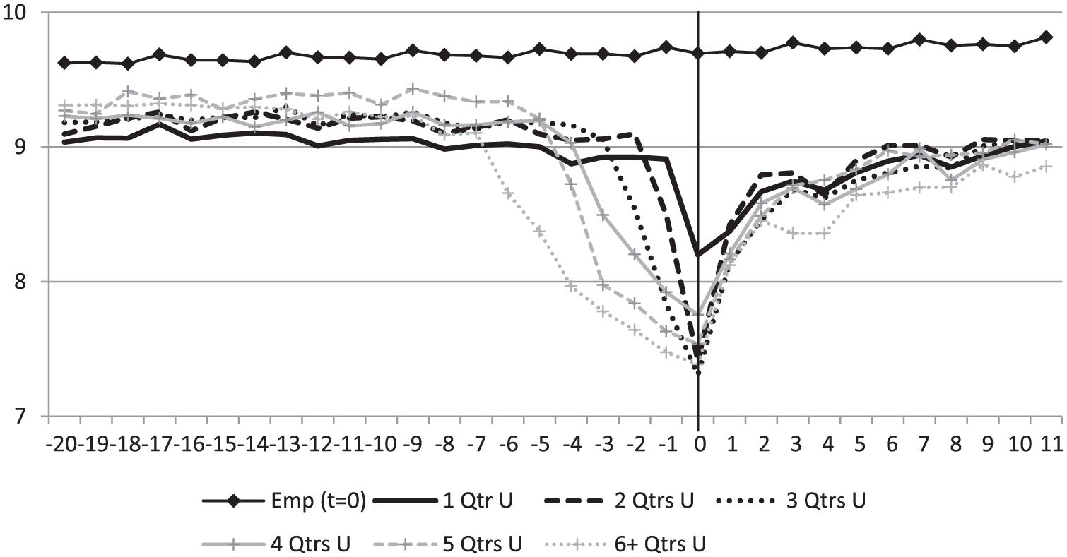
Real Earnings (IHS Earnings > 0)
The profiles plotted in Figure 2A are similar in appearance to the employment probability profiles we have already discussed. The profiles plotted in Figure 2B look quite different. Even among those with positive earnings, those who were employed at q = 0 have higher average IHS (real earnings) both before and after q = 0 than those in any of the unemployment by duration groups. Conditional on having a UI job, however, the differences in the earnings of the short-duration and long-duration unemployed are relatively modest. 8
Note that an identity links Figure 1 and the two panels of Figure 2. Since IHS(0)=0, the measure of earnings reported in Figure 2A for a given duration group and quarter is equal to the probability of being employed in that group and quarter in Figure 1 times the measure of earnings reported in Figure 2B for that same group and quarter. This identity along with the relatively small differences in Figure 2B compared to Figure 2A implies that most of the difference in earnings outcomes across unemployment duration groups apparent in Figure 2A occurs along the extensive margin (whether people are employed in a quarter) rather than along the intensive margin (how much they earn if they work). We explore this issue more systematically in the next section of the article.
Regression Results
Although a great deal can be learned from Figure 1 and Figure 2, visual inspection of the data takes us only so far. We turn now to a regression analysis that allows us to test for the statistical significance of observed pre-spell and post-spell differences across the duration groups, controlling for other factors that may differ across them. As noted, our methodology borrows from the related literature on job displacement, which grew out of a similar interest in learning about the effects of an event (in that case, job displacement) on subsequent labor market outcomes.
Estimation Framework
Rather than including all available quarters of data, the regression models we have estimated focus on employment and earnings eight quarters prior to and eight quarters following the CPS link quarter (q = 0). Begin by considering the following simple specification:
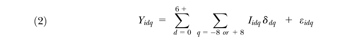
where d = {0, 1, 2, … 5, 6+} indexes the employment or unemployment duration group to which a person belongs, with d = 0 representing people who are CPS employed and d > 0 representing people with different unemployment durations in the CPS as of the CPS-LEHD link quarter; q =–8 or +8 indexes the quarter either eight quarters before or eight quarters after the link quarter, and i indexes the person-year observation. We suppress calendar year time indices for convenience. Although this is not written out explicitly, we think of the
Estimating Equation (2) by ordinary least squares (OLS) yields estimated
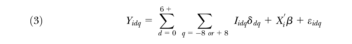
where the

We also want to allow, however, for the possibility of fixed but unobservable differences in individuals’ underlying employment propensities. To do this, we focus on estimates of:

This loss is the change in the employment rate or in the mean of IHS(real earnings) from eight quarters before to eight quarters after q = 0 for a given unemployment duration group. Note that any fixed effects associated with either observable or unobservable individual characteristics that might have contributed to differences in the estimated

Equation (6) provides an estimate of the differential effect of being long-term unemployed rather than short-term unemployed on the outcome of interest that is uncontaminated by the influence of any time-invariant individual effects on that outcome.
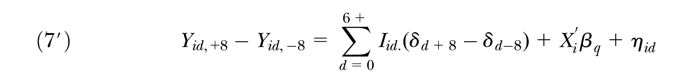
As just described, the estimates of interest may be obtained by fitting Equation (3) directly, using the (potentially biased)
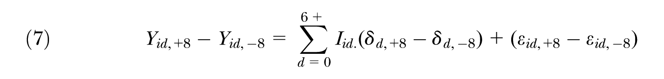
where Iid. is a dummy variable that equals 1 if the observations being differenced pertain to duration group d, and otherwise equals 0. Observe that any time-invariant individual controls are eliminated in this specification, along with the effects of any fixed but unobserved individual heterogeneity. The two approaches are demonstrably equivalent and will yield identical point estimates of the LossN and LossDiffN1 effects of interest. The results we report are based on estimates of Equation (3), but the interpretation of the specification shown in Equation (7) may in some ways be more intuitive.
By focusing on the losses in Equation (5) and the differences in losses in Equation (6), we are controlling for fixed factors affecting individuals’ employment and earnings propensities. These estimates do not, however, control for possible differences in employment and earnings trajectories across individuals. Age is one possible source of differences in employment trajectories. Life cycle dynamics imply that we should expect upward-sloping employment and average earnings profiles for those at younger ages, as more of them complete their education and enter the labor force, and downward-sloping employment and average earnings profiles for older age groups, reflecting the gradual withdrawal of group members from the labor force. Figure A.4 in the Online Appendix contains plots similar to Figure 1 but broken out by age group (less than 30 years, 30–49 years, or 50-plus years); there is a clear upward slope to the measured employment probabilities for the under-30 age group that is not present in the figures for the two older age groups. To control for such factors we consider a modified version of Equation (3) given by:
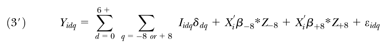
where
where
As already noted, all of the included Xs in these specifications are fixed across the two data points related to each person-year CPS observation. The demographic controls available to us include gender, age (15–24, 25–34, 35–44, 45–54, 55–64, 65+), education (less than high school, high school graduate, some college, college graduate, graduate degree), race (white, black, other), marital status, and foreign born, all defined as of the date of the CPS link quarter (q = 0). Models estimated with demographic controls also include year dummies. In addition, we make use of the previously described job history and employment trajectory variables derived from the employment histories contained in the LEHD data infrastructure.
Employment Equation Estimates
Estimates of the δ parameters from a set of linear probability models with an indicator for whether the person is employed as the dependent variable are reported in the top two panels of Table 2. The q =–8 parameters for the employment and six unemployment duration groups are reported in the top panel of the table; the q =+8 parameters for the same groups are reported in the second panel. The next three panels report the DiffN1, LossN, and LossDiffN1 estimates computed from those δ values. To conserve space, we do not report standard errors, but note that given the large samples, all of the estimated δ parameters are estimated with considerable precision. The model in column (1), based on Equation (2), includes only dummy variables for duration group (d = 0 for the employed and d = 1, 2, 3, 4, 5, or 6+ for the unemployed) by quarter (q =–8 or q =+8). The models in columns (2) and (3), based on Equation (3), add demographic controls and year effects (column (2)) and the share of quarters q = {–20,–9} during which the person had UI employment (column (3)). The models in columns (4), (5), and (6) are based on Equation (3′). Column (4) includes demographic and year effects; column (5) adds the previously described q = {–20,–9} job history variable; and column (6) adds the employment trajectory control also based on q = {–20,–9}. Recall that Equation (3′) differs from Equation (3) in allowing the coefficients on the various control variables to differ across the pre-link and post-link quarters. 11
Employment Probability Regressions
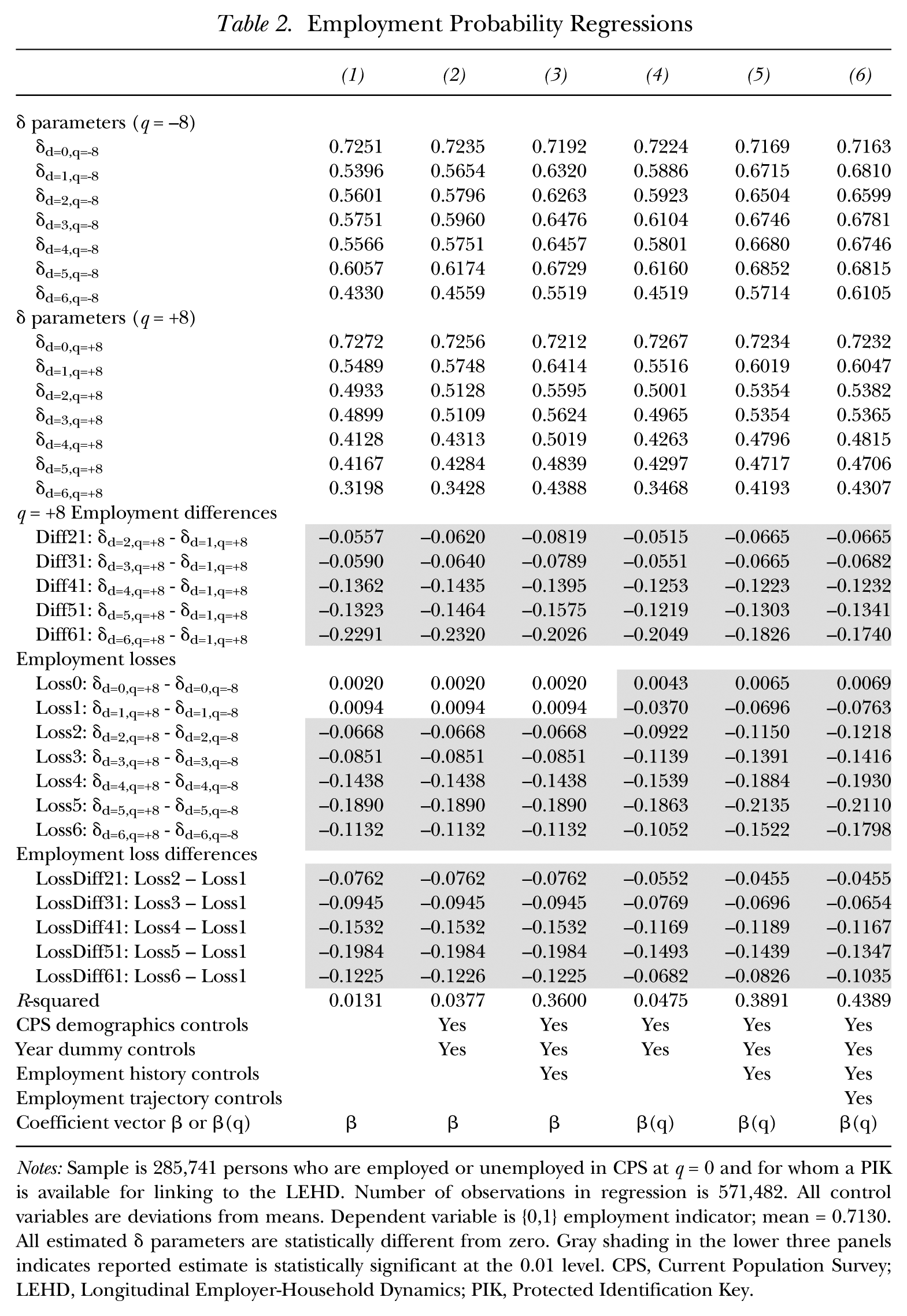
Notes: Sample is 285,741 persons who are employed or unemployed in CPS at q = 0 and for whom a PIK is available for linking to the LEHD. Number of observations in regression is 571,482. All control variables are deviations from means. Dependent variable is {0,1} employment indicator; mean = 0.7130. All estimated δ parameters are statistically different from zero. Gray shading in the lower three panels indicates reported estimate is statistically significant at the 0.01 level. CPS, Current Population Survey; LEHD, Longitudinal Employer-Household Dynamics; PIK, Protected Identification Key.
The parameter estimates in column (1) of the top two panels of Table 2 simply reproduce the employment probability values for q =–8 and q =+8 that can be read off the plot displayed in Figure 1. In both q =–8 and q =+8, the probability of UI employment for people who are CPS employed in the link quarter (q = 0) are substantially higher than the corresponding probabilities for people who are unemployed. 12 Except for the group unemployed six quarters or more, the q =–8 employment probability differs little across the unemployment duration groups; at q =+8, however, the probability of having UI employment is notably lower for those with longer q = 0 unemployment durations. To illustrate, those unemployed five quarters at q = 0 have a UI employment rate in q =+8 that is 13.2 percentage points below the UI employment rate for those unemployed just one quarter at q = 0 (UI employment rate of 41.7% versus 54.9%). As indicated by the gray shading, all of the differences in q = +8 employment rates between those in the longer unemployment duration groups compared to those in the one-quarter duration group are statistically significant at the 0.01 level.
The models reported in columns (2) and (3) of Table 2 contain additional controls but constrain their coefficients to be the same in q =–8 and q =+8. The addition of these controls—demographic and year effects in column (2) and, especially, job history controls in column (3)—raises the estimated q =–8 and q =+8 employment probabilities for all of the unemployment duration groups. In other words, had the observable characteristics of the unemployed been the same as those of the average person in the linked sample, both their q =–8 and their q =+8 employment rates would have been somewhat higher. 13 We are more interested, however, in what the models that include these added controls imply about the difference in the impact of being long-term unemployed rather than short-term unemployed on subsequent employment.
One way to approach this question, similar to the analysis in KCC (2014), is simply to compare the estimated
As already discussed, one potential problem with the DiffN1 estimates based simply on the
To illustrate, consider the estimated losses and differences in losses shown in column (2) of Table 2. Similar to KCC (2014), this model controls for demographics and year. Other than for the six-plus-quarter group, the loss differences are all somewhat larger than the simple differences in the
Note that, by construction, starting with a model that has no controls and then introducing time-invariant control variables whose coefficients are constrained to be the same in both q =–8 and q =+8 will have no effect in a balanced panel on the estimated employment losses or loss differences across the two periods. This result can be seen in the LossNs and LossDiffN1s reported in the first three columns at the bottom of Table 2, which are identical across the columns.
The models in columns (4), (5), and (6) of Table 2 allow for the coefficients on the various control variables to differ across the pre-link (q = −8) and post-link (q = +8) quarters. This approach has a large effect on several of our estimates. For example, for the individuals who have one quarter (1–13 weeks) of unemployment in the link quarter, the estimates in the three right-hand columns show sizeable losses in employment (a 3.7 percentage point loss in column (4), a 7.0 percentage point loss in column (5), and a 7.6 percentage point loss in column (6)), rather than the small gains shown in columns (1) through (3). This finding occurs because many of the short-duration unemployed are young adults—people who are more likely than the average to have been in school rather than working two years earlier and to be working two years later. Taking into account this underlying dynamic and its implication that, based on their demographics, the employment rates for the short-term unemployed should be higher in q =+8 than in q =–8 makes the post-unemployment outcomes of the short-term unemployed look relatively worse. As a result, the differences in losses between the long-term unemployed and the short-term unemployed are smaller (in absolute value) in the models that allow for time-varying coefficients on the control variables. In column (2) of Table 2, for example, the reported difference in losses between those who are unemployed five quarters (53–65 weeks) at the time of their CPS interview and those unemployed just one quarter (1–13 weeks) is 19.8 percentage points; in the corresponding model in column (4) that allows the coefficients on the same included control variables to vary with time, this difference falls to 14.9 percentage points.
In summary, the employment probability regression results in Table 2 quantify the patterns that were evident in Figure 1. First, individuals who report CPS-LEHD link quarter CPS employment are substantially more likely to have UI employment eight quarters prior to the link quarter than any of the unemployed groups. Further, the corresponding pre-unemployment UI employment rates are similar for persons with unemployment durations of one to five quarters. Eight quarters after the CPS-LEHD match, those who report being unemployed in the CPS are less likely to be employed, and this is especially true for those who had been unemployed longer at the time of the CPS interview. The inverse relationship between unemployment duration and subsequent employment rates holds even after controlling for time-invariant unobservable heterogeneity and for pre-unemployment heterogeneity in employment trajectories. Our findings thus are consistent with negative duration dependence in the rate of exit to employment across a spell of unemployment—that is, with extended unemployment being the cause of the poorer subsequent employment outcomes experienced by the long-term unemployed.
Role of Labor Market Shocks and External Labor Market Conditions
Although our results permit us to dismiss observed and unobserved time-invariant heterogeneity across individuals as an explanation for the strong association between long-term unemployment and lower employment probabilities, the poorer job-finding prospects of the long-term unemployed could alternatively be a consequence of their having experienced especially adverse labor market shocks or especially negative external labor market conditions rather than being attributable to their extended unemployment. Although we cannot entirely rule out this explanation, two pieces of evidence suggest that it is unlikely to fully account for our findings.
First, when we look separately at the data broken out by reason for unemployment, we observe a relationship between unemployment duration and subsequent employment rates that is very similar to that in the full unemployed sample. Holding reason for unemployment constant is a rough way to control for differences in the nature of the shocks that individuals have experienced. As can be seen by comparing across the three panels of Online Appendix Figure A.5, job losers at every unemployment duration fare worse with respect to subsequent employment than those who quit their previous jobs or are just entering the labor force, suggesting that as a group job losers have experienced more negative shocks than those in the other reason-for-unemployment groups. Among job losers, however, it remains the case that employment losses are notably larger for the long-term unemployed than for the short-term unemployed. Further, the differences in employment losses across unemployment duration groups in the job-loser population are very similar to the corresponding differences in the full unemployed population. 14 If the differential employment losses for the long-term versus the short-term unemployed were being driven primarily by differences in the events leading to their unemployment, we would have expected the differences across unemployment duration groups to be smaller within the job-loser population, but this is not what we observe.
As a second sensitivity check, we constructed variables intended to capture differences in the external labor market conditions experienced by different members of our sample and added these variables to the models reported in Table 2, then examined how this affected the estimated employment losses across unemployment duration groups. First, using data from the QCEW, we constructed a measure equal to the percentage change in overall employment in a person’s state between q = −8 and q = +8. Second, we modified this variable by substituting, for those who had been employed at q = −8, the percentage change in employment in the person’s 6-digit North American Industry Classification System (NAICS) industry and state between q = −8 and q = +8. 15 Both of these employment change variables were more negative for those who were unemployed at q = 0 than for those who were employed and, generally speaking, for those among the unemployed with a longer duration of unemployment. To give a sense of magnitudes, the average state employment change over the q = −8 to q = +8 period ranges from –0.3% for the one-quarter unemployment group to –2.4% for those in the five-quarter unemployment group; the corresponding range in the values for the state-by-industry version of the employment change variable is from –4.2% to –8.5%.
The effects of including these variables in our employment regressions are shown in Online Appendix Tables A.1 and A.2; models that allow the state-by-industry employment growth variables to affect those employed at q = 0 differently from those unemployed at q = 0 are shown in Online Appendix Table A.3. Adding the employment change variables has almost no effect on the relative probabilities of employment at q =+8 or, more important, on the estimated differences in employment losses by unemployment duration group. Although those experiencing poorer external labor market conditions appear to have suffered more negative employment changes between q = −8 and q = +8, the differences in labor market conditions experienced by the long-duration and short-duration unemployed as captured by these variables are not large enough to explain any material part of the difference in job-finding rates or the difference in employment losses between the long-duration and the short-duration unemployed.
Earnings Equation Estimates
Estimates of the δ parameters from two sets of earnings models are reported in the top two panels of Table 3 and Table 4. The model in Table 3 (which corresponds to Figure 2A) is fit using data for everyone in the sample whether they have earnings in a given quarter or not; in quarters with no UI earnings, a 0 is assumed. The model in Table 4 (which corresponds to Figure 2B) uses only those observations for which positive UI earnings are reported in the quarter. In both cases, as already described, the dependent variable is IHS(real earnings). The structure of the tables reporting on the earnings models is the same as the structure of the employment probability table just discussed. The only difference in model specification is that in columns (3), (5), and (6), employment history and employment trajectory variables based on q = {–20,–9} are replaced with the earnings history and earnings trajectory variables that correspond to the model’s dependent variable. In column (6), the indicator variable for whether the earnings trajectory measure could be constructed also is included. 16
Earnings Regressions (IHS, Earnings ≥ 0)
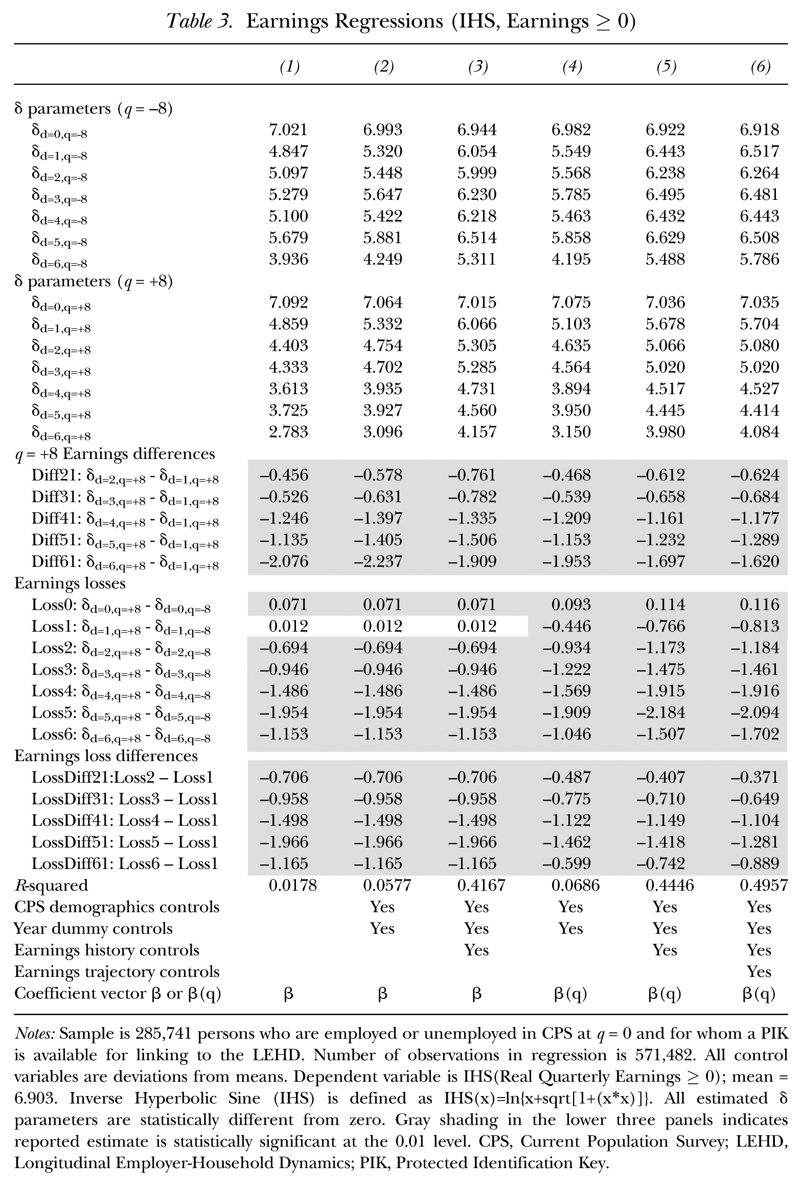
Notes: Sample is 285,741 persons who are employed or unemployed in CPS at q = 0 and for whom a PIK is available for linking to the LEHD. Number of observations in regression is 571,482. All control variables are deviations from means. Dependent variable is IHS(Real Quarterly Earnings ≥ 0); mean = 6.903. Inverse Hyperbolic Sine (IHS) is defined as IHS(x)=ln{x+sqrt[1+(x*x)]}. All estimated δ parameters are statistically different from zero. Gray shading in the lower three panels indicates reported estimate is statistically significant at the 0.01 level. CPS, Current Population Survey; LEHD, Longitudinal Employer-Household Dynamics; PIK, Protected Identification Key.
Earnings Regressions (IHS, Earnings > 0)
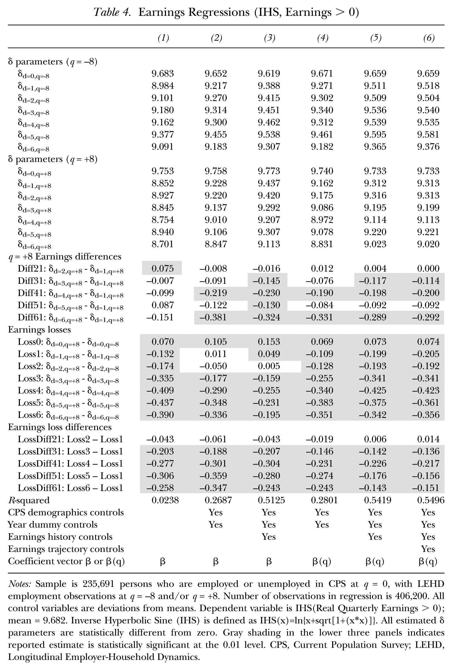
Notes: Sample is 235,691 persons who are employed or unemployed in CPS at q = 0, with LEHD employment observations at q = −8 and/or q = +8. Number of observations in regression is 406,200. All control variables are deviations from means. Dependent variable is IHS(Real Quarterly Earnings > 0); mean = 9.682. Inverse Hyperbolic Sine (IHS) is defined as IHS(x)=ln{x+sqrt[1+(x*x)]}. All estimated δ parameters are statistically different from zero. Gray shading in the lower three panels indicates reported estimate is statistically significant at the 0.01 level. CPS, Current Population Survey; LEHD, Longitudinal Employer-Household Dynamics.
The estimates that appear in Table 3 are in many respects very similar to those in Table 2. Looking at the full linked sample, at q =–8, the IHS(real earnings) of those who will be employed in the CPS at q = 0 are significantly higher than those for any of the groups that will be unemployed in q = 0. The point estimates of the coefficients for the q =–8 measure of earnings across the first five unemployment duration groups are generally similar. At q =+8, it continues to be the case that those who were employed in the CPS at q = 0 have higher IHS(real earnings) than those in any of the unemployment duration groups, but now those with longer unemployment durations at q = 0 have earnings that are systematically lower than those with shorter unemployment durations at q = 0. Looking at the LossN statistics in column (1), the quarterly earnings of employed individuals rise on average between q =–8 and q =+8, and quarterly earnings for the group unemployed 1–13 weeks as of the link quarter do not change significantly. By contrast, quarterly earnings for all of the longer-term unemployment groups exhibit a significant decline, and the magnitude of these earnings losses increases monotonically with unemployment duration through the group with five quarters of unemployment at the link quarter; the losses of those unemployed six-plus quarters are smaller because that group was doing poorly even at q =–8.
Controls for demographics and year are added in column (2); those variables plus a measure of the individual’s earnings history over the period q = {–20,–9} appear in column (3). In these models, the coefficients on the added variables are constrained to be the same in q =–8 and q =+8. The same variables are added in column (4) and column (5) but with their coefficients permitted to differ across the two periods. Column (6) controls for the q = {–20,–9} earnings trajectory as previously described, along with an indicator variable for those for whom this trajectory could not be constructed. As before, by construction, adding fixed controls with coefficients constrained to be equal across the two time periods may raise or lower the level of the estimated δs but by the same amount in both q =–8 and q =+8, so that the estimated LossNs are not affected. This is why the losses reported in column (2) and column (3) are identical to those reported in column (1). To affect the estimated losses, the coefficients on these variables must be allowed to differ across time periods so they can pick up differences in the earnings trajectories associated with observable characteristics that might be correlated with unemployment duration. When this is done in columns (4), (5), and (6), we observe larger estimated earnings losses for several of the unemployment duration groups (those with one to four quarters of unemployment as of the date of the CPS-LEHD match). The implication is that, given the characteristics of the members of these groups, their earnings would have been expected to grow and the declines actually experienced between q =–8 and q =+8 look worse relative to this expected-growth benchmark than relative to the no-change benchmark implicit in column (1).
Table 4 repeats this exercise conditional on positive earnings in q =–8 and q =+8. We undertake this exercise to take advantage of the identity noted above in our discussion of Figures 1 and 2. The following identity relates the top two panels of Tables 2, 3, and 4:

where the numbered superscripts reference the table number. That is, for duration group d and quarter q, the estimated overall mean of IHS(real earnings) in Table 3 denoted by
One caution in interpreting the results in Table 4 in isolation is that the estimation of Equation (3) and Equation (3′) is no longer based on a balanced panel of observations for individuals who have an unemployment spell in a given reference year. The reason is that the dependent variable is contingent on positive earnings in a given quarter. As such, the estimated losses from taking the differences in the top two panels of Table 2 are no longer equivalent to the losses estimated from first-difference specifications (7) and (7′). With this caveat in mind, we note that the qualitative patterns of Table 4 are similar to those in Table 3 but the quantitative impacts are substantially reduced. Even with smaller magnitudes, the estimated earnings loss effects are still substantial. For example, in column (6) of Table 4 in the bottom panel, among those who have earnings, the differential earnings loss between q =–8 and q =+8 for the long-term (five quarter) unemployed compared to the short-term (one quarter) unemployed is approximately 16 ln points (given that the differences in the IHS values are approximately ln differences at the values reported in Table 4).
The identity in Equation (8) permits an exact decomposition of the earnings losses in Table 3:

where
Concluding Remarks
The sharp rise in long-term unemployment during the Great Recession and the slow subsequent recovery have heightened concerns about the distressingly bad labor market outcomes experienced by the long-term unemployed. Efforts to form a clear understanding of the reasons for this group’s persistently lower subsequent employment rates and earnings levels have long been plagued, however, by the challenge of distinguishing the effects of state dependence from those of unobserved heterogeneity, in particular the possibility that the long-term unemployed are individuals whose employment probabilities and earnings outcomes would have been worse than those of the short-term unemployed even absent their experience of extended unemployment.
We use integrated survey and administrative data to overcome this challenge. From the CPS, we identify currently unemployed individuals who have been unemployed for different lengths of time. We integrate these survey data with matched employer–employee data from the LEHD data infrastructure. This approach enables us to generate employment and earnings profiles for those in a current spell of unemployment over an interval from 20 quarters prior to 11 quarters after the date they are observed as unemployed in the CPS.
Using these integrated survey and administrative data, we evaluate the impact of the duration of unemployment through the lens of differences in the pre-spell and post-spell employment and earnings outcomes. More specifically, our linked data enable us to control for fixed effects attributable to individual characteristics measured as of the date an unemployed person is observed in the CPS as well as fixed effects attributable to unobserved but unchanging individual characteristics. For a given group of individuals, any such effects should affect both the pre-spell and post-spell employment and earnings outcomes in the same way, allowing us to draw meaningful inferences from the differences in the pre-spell and post-spell outcomes for a given duration group. In turn, we consider how these differences vary across duration groups. We find that, even after accounting for differences in their observed and unobserved characteristics, the long-term unemployed experience employment and earnings losses that are substantially greater than those experienced by the short-term unemployed.
This fixed-effects approach does not control for different employment trajectories across individuals that might be driving differences across unemployment duration groups. Given our integrated survey and administrative data set, we are able to control for differences in trajectories associated with observable characteristics and, at least to some extent, for differences in trajectories observable in each individual’s own history. Controlling for such trajectories somewhat mitigates the differences in employment and earnings losses between the long-term and short-term unemployed, but they remain substantial.
These results allow us to rule out the “bad apple” explanation for why the long-term unemployed fare worse in the labor market than do the short-term unemployed and are consistent with duration dependence as the explanation for their poorer outcomes. It is possible that differences in the labor market shocks or external labor market conditions experienced by the long-term and the short-term unemployed could explain at least a portion of the differences we have documented. Two pieces of evidence suggest this is unlikely to be the whole story. First, we observe very similar patterns even when the sample is restricted to those who entered unemployment due to the loss of a job. Further, controlling for employment growth rates in an individual’s state or in their state and industry as a means of capturing differences in the labor market conditions to which a person has been exposed has almost no effect on the estimated difference in outcomes between the long-term and the short-term unemployed. Although this evidence provides additional reason to think that extended unemployment is itself a cause of negative outcomes, there would certainly be value in a more complete exploration of the possible role of differential shocks or differences in external labor market conditions as contributing factors.
Using much the same approach as just described for studying the effect of long-term unemployment on subsequent employment, we also examine the impact of unemployment duration on subsequent earnings. We document a significant adverse impact of long-term unemployment as compared to short-term unemployment on what individuals later earn. Most of this effect is realized through the extensive margin, that is, through its effect on the probability of being employed. The long-term unemployed do experience greater earning losses conditional on being employed, but the large majority of the adverse impact of long-term unemployment on earnings takes place along the extensive margin.
An important avenue for future research will be to develop a better understanding of the relative importance of the specific factors that may be contributing to duration dependence in the effects of unemployment on later employment and earnings—including human capital depreciation during spells away from work, decreases in search intensity over the spell of unemployment, and employer discrimination against the long-term unemployed in hiring, among other possibilities.
Our findings highlight the advantages of integrated survey and administrative data for questions related to the consequences of passing through a spell of unemployment. There is no obvious way to identify and track spells of unemployment (as opposed to non-employment) in administrative data. The primary source for information on unemployment is the CPS, but the CPS contains limited information on the experiences of unemployed workers prior to or following their unemployment spell. Integration of administrative data such as that from the LEHD data infrastructure with the CPS records permits the construction of employment and earnings histories that greatly enhance what can be said about the consequences of being unemployed.
Supplemental Material
DS_10.1177_0019793918797624 – Supplemental material for The Consequences of Long-Term Unemployment: Evidence from Linked Survey and Administrative Data
Supplemental material, DS_10.1177_0019793918797624 for The Consequences of Long-Term Unemployment: Evidence from Linked Survey and Administrative Data by Katharine G. Abraham, John Haltiwanger, Kristin Sandusky and James R. Spletzer in ILR Review
Footnotes
Acknowledgements
We thank Lucia Foster, Henry Hyatt, Robert Valletta, Till von Wachter, and an anonymous referee for helpful comments and suggestions. We also have benefited from the opportunity to present earlier versions of the paper at the U.S. Census Bureau, Princeton University, the Institute of Labor Economics (IZA), the Society of Labor Economists Annual Meetings, and the Econometric Society Winter Meetings.
Any opinions and conclusions expressed herein are those of the authors and do not necessarily represent the views of the U.S. Census Bureau. All results have been reviewed to ensure that no confidential information is disclosed.
For information regarding the data and/or computer programs used for this study, please address correspondence to the lead author at
1
The 31 states are California, Colorado, Connecticut, Florida, Georgia, Hawaii, Idaho, Illinois, Indiana, Kansas, Louisiana, Maine, Maryland, Minnesota, Missouri, Montana, Nevada, New Jersey, New Mexico, North Carolina, North Dakota, Oregon, Pennsylvania, Rhode Island, South Carolina, South Dakota, Tennessee, Texas, Washington, West Virginia, and Wisconsin.
2
More specifically, for each year, we estimate a regression model in which an indicator for having a PIK is regressed on indicators for age group, gender, race, education, marital status, foreign-born status, and whether the person reported being employed in the relevant March CPS. We use the coefficients from this model to calculate each individual’s probability of having a PIK, and then apply a weight adjustment equal to the inverse of this probability to the CPS monthly estimation weight. Individuals with a PIK are retained in our sample regardless of whether we are able to locate any employment records for them in the LEHD data.
3
For example, with the 2008–2010 CPS sample, the employment probability eight quarters later for individuals unemployed five quarters as of the CPS interview date is 41.6% when computed using UI job data for 31 states, and 42.5% when computed using UI job data for 48 states. The effects of shifting from estimates based on UI data for 31 states to estimates based on UI data for 48 states are similarly small and very similar in magnitude for each of the other unemployment duration groups.
4
Burbidge, Magee, and Robb (1988) and ![]() described the advantages of the IHS transformation.
described the advantages of the IHS transformation.
5
The negative trajectories for those in the group with six or more quarters of unemployment at q = 0 may be an artifact of some of these individuals having begun their spell of unemployment toward the end of the q = {–20,–9} period.
6
In addition, someone who lives in one of our 31 CPS states could be employed in a jurisdiction not covered by our data. For example, a Maryland resident included in our 31 state sample might be employed in the District of Columbia or Virginia, jurisdictions for which we do not have UI data. As already discussed, however, this appears to have only a relatively minor effect on our estimates.
7
There could be a small number of people who were unemployed during the March CPS reference week but then subsequently found a job and received a first paycheck on that job before the end of the month, meaning that they would have had an unemployment insurance wage record for the first quarter of the year. Given that the March CPS reference week covers the period through March 15 on average, however, we would expect this to be a relatively rare event. Employment during the q = 0 quarter for those unemployed 13 weeks or less is not surprising, as these unemployment spells would have begun during that quarter. Similarly, employment during the q =–1 quarter is not surprising for those unemployed 14–26 weeks, employment during the q =–2 quarter is not surprising for those unemployed 27–39 weeks, and so on.
8
The top and bottom panels of Figure 2 have different scales along the vertical axis, chosen to span the values plotted in each. Online Appendix Figure A.3 presents the top and bottom panels on consistent scales, meaning that a visual comparison of the panels shows directly how much of the earnings variation across duration groups is attributable to the extensive margin (employment versus non-employment) compared to the intensive margin (earnings variation conditional on employment). Note that Figure 2A is based on a balanced panel for each reference spell, whereas ![]() includes only those for a given reference spell with positive earnings in a particular quarter.
includes only those for a given reference spell with positive earnings in a particular quarter.
9
For example, for the q =–8 observation for a person in unemployment duration group 3, Ii3,–8 would equal 1 and all of the other Iidq variables would equal 0.
10
Although the coefficients estimated in ![]() are subject to omitted variable bias stemming from the omission of time-invariant individual effects, given that we are working with a balanced panel for each reference year, this bias is of the same size and magnitude for
are subject to omitted variable bias stemming from the omission of time-invariant individual effects, given that we are working with a balanced panel for each reference year, this bias is of the same size and magnitude for
11
In sensitivity analyses available upon request, we considered models that added the full complement of previously described earnings history and earnings trajectory variables for the period q = {–20,–9} to the employment history and employment trajectory variables included in models (3), (5), and (6) of ![]() . This approach had very little effect on the estimated coefficients and did not change any of our qualitative conclusions.
. This approach had very little effect on the estimated coefficients and did not change any of our qualitative conclusions.
13
Because our sample contains so many more employed people than unemployed people, the characteristics of the full sample are very similar to the characteristics of the employed population.
14
The changes in the employment rate between q = −8 and q = +8 in the full sample are 7.6 percentage points, 9.4 percentage points, 15.3 percentage points, 19.8 percentage points, and 12.2 percentage points more negative among those who are two-quarter, three-quarter, four-quarter, five-quarter, and six-quarter unemployed at q = 0, respectively, than for those who are one-quarter unemployed at q = 0. The corresponding numbers for those unemployed due to job loss are 6.6 percentage points, 14.3 percentage points, 15.4 percentage points, 20.9 percentage points, and 9.1 percentage points.
15
We also constructed an indicator taking the value of 1 if a person had been employed at a firm with 50 or more employees as of quarter d at which a mass layoff had occurred in the surrounding quarters, defined as a drop in employment of 30% or more between quarter d–1 and d, d and d+1 or d–1 and d+1. As there was no systematic relationship between the value of the mass layoff indicator and unemployment duration, we did not pursue any further analysis with that variable.
16
In sensitivity analyses available upon request, we considered models that added all of the employment history and employment trajectory variables for the period q = {–20,–9} to the earnings history and earnings trajectory variables corresponding to the dependent variable that are included in the models reported in columns (3), (5), and (6) of Table 3 and ![]() . Doing this had very little effect on the estimated coefficients and did not change any of our qualitative conclusions.
. Doing this had very little effect on the estimated coefficients and did not change any of our qualitative conclusions.
17
The identity in Equation (8) is exact for column (1) of Tables 2, 3, and 4. The addition of control variables to the models reported in those tables breaks the exact identity, but the resulting “error” is small. Defining error as the absolute value of the difference between the δ estimates shown in ![]() and those calculated using Equation (8), this error never exceeds 5% of the actual δ estimates in Table 3.
and those calculated using Equation (8), this error never exceeds 5% of the actual δ estimates in Table 3.
References
Supplementary Material
Please find the following supplemental material available below.
For Open Access articles published under a Creative Commons License, all supplemental material carries the same license as the article it is associated with.
For non-Open Access articles published, all supplemental material carries a non-exclusive license, and permission requests for re-use of supplemental material or any part of supplemental material shall be sent directly to the copyright owner as specified in the copyright notice associated with the article.