Efficient predictive cruise control of autonomous vehicles with improving ride comfort and safety

Abstract

In this paper, the adaptive cruise control problem of autonomous vehicles is considered and we propose a novel predictive cruise control approach to improve driving safety and comfort of the host vehicle. The main idea of the approach is that the predicted acceleration commands of the host vehicle are stair-likely pre-planned to satisfy their changes along the same direction within the prediction horizon. The predictive cruise controller is then computed by online solving a finite horizon constrained optimal control problem with a decision variable. Besides explicitly handling safety constraints of vehicles, the obtained controller has abilities to efficiently attenuate peaks of the cruise commands while reducing computational load of online solving the optimization problem. Hence, the ride comfort and safety performances of vehicles are improved in terms of softening acceleration response and constraint satisfaction. Moreover, the ride comfort, following and safety performances of vehicles are summed with varying weights to cope with various traffic scenarios. Some classical cases are adopted to evaluate the proposed adaptive cruise control algorithm in terms of ride comfort, car-following ability and computational demand.

Keywords

Adaptive cruise control model predictive control constrained control ride comfort

Introduction

The adaptive cruise control (ACC) technology has been adopted by many road vehicles, for example, passenger cars and heavy trucks. The advantages of ACC are to lessen drivers’ burden and raise driving safety by adjusting the velocity and/or a safe inter-vehicle distance (i.e. spacing) between the host vehicle and its preceding vehicle.¹ Due to the increasing strict environment and ride comfort concerns, the ACC systems are required to be able to achieve more functionality (objectives) including safety, following, ride comfort and fuel economy.^2–4 In general, the multiple objectives of the ACC system are conflicting with each other. Many efforts have been made to deal with these conflicting objectives in the last decades.

In view of the car-following performance, the authors in Zhang and Ioannou⁵ employed the proportional–integral–derivative (PID) method to evaluate the performance by taking into account different spacing polices. Moreover, the particle swarm optimization, genetic algorithm, sliding mode control and back-stepping control were used to maintain the spacing of two adjacent vehicles.^5–8 By the invariant-time headway strategy, a fuzzy neural cruise controller was trained to imitate human spacing adjustment behaviors.⁹ Moreover, it is known that the smooth responses of cars are benefit to improve fuel saving and ride comfort of cars.⁵ Hence, Naus et al.¹⁰ and Ahmed and Svaricek¹¹ limited the vehicle’s acceleration level and then developed filter-based ACC and offline dynamic programming–based ACC methods to satisfy fuel saving and ride comfort concerns. In Kim et al.,¹² the virtual leading vehicle strategy was used to achieve smoother responses compared with the traditional mode switching schemes. These methods efficiently improve ride comfort of the host vehicle at the sacrifice of car-following ability. Because the quick car-following ability generally implies some drastic changes in the acceleration profile and its derivative (jerk) of the host vehicle.

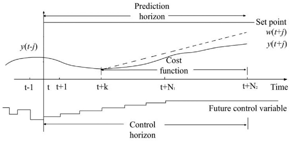
Model predictive control (MPC) provides an alternative framework to reconcile the contradictory of the multiple objectives of ACC,^{3–4,10–13} which forms the so-called predictive cruise control (PCC) method. In general, MPC actions are determined by online solving a finite horizon optimization problem where the cost function penalizes deviations of evolutions of a system with respect to its target behavior. Then the first action of the control sequence calculated is applied to the system and the procedure is repeated at the next time in a receding horizon manner.^14,15 Due to its ability to explicitly handling constraints and optimization, MPC has been attracting great attention in automotive applications in recent years.^16–20

In PCC, the multiple objectives are generally summed as an optimization objective by selecting a set of appropriate weights. Then a finite horizon open-loop optimal control problem is solved online to minimize the resulted objective function within the vehicle dynamics and driving safety constraints. For example, the authors in Sancar and Huissoon²¹ adopted MPC to replace PID structure to satisfy ACC functionalities and avoid rear-end collisions. In Sina and Wahde,²² the velocity of heavy-duty vehicles was optimized to reduce the fuel consumption in the MPC framework and in Bijan et al.,²³ the authors presented an ecological PCC system by taking account of traffic-light-to-vehicle to predict the future trajectories of the host vehicle.²⁴ In Moser et al.,²⁵ a stochastic PCC algorithm was presented to minimize the fuel consumption, together with a short-term predicting the predecessor’s speed. Liu et al.²⁶ and Shakouri et al.²⁷ used PCC to minimize the energy consumption of hybrid electric cars. To achieve safety and satisfied car-following ability, Kohut et al.²⁸ presented a hybrid PCC method and Lin et al.²⁹ proposed a neuro-fuzzy PCC algorithm to minimize car-following errors. Moreover, Hellström et al.³⁰ presented the PCC strategy to compromise fuel efficiency and trip time within a given speed range by optimizing the engine torque. By the weighted-sum method, previous studies^3–4,12 presented multi-objective PCC to make a trade-off between ride comfort, fuel economy, safety and car-following ability. Rather than using the invariant weights,⁴ a multi-objective PCC algorithm with varying weights was proposed by Zhao et al.³¹ to accommodate various traffic scenarios. The main merit of PCC is its ability to explicitly tackle various constraints of ACC in the optimization control framework. In available PCC applications, the ranges of acceleration commands of the host vehicle are often bounded in prior in order to improve ride comfort and fuel efficiency. However, these limitations are not necessary to yield smooth responses of the ACC system as changes in vehicular acceleration commands may be drastic. As a result, vehicles ride comfort cannot be improved by bounded acceleration commands. In addition, the available PCC algorithms have not considered the computational burden of online solving the optimization problem of PCC yet during design of the vehicular ACC systems.

It is well known that a dynamic system yields smoother responses when it is driven by a smooth control input.³² Moreover, the computational demand of MPC increases exponentially to the number of degrees of freedom in the predicted control sequences.³³ In this paper, we focus on the PCC problem as well as the computational burden of the PCC controller. Based on some constrained incremental models of vehicular ACC systems, we propose a new PCC algorithm to the ACC system. The predicted acceleration commands of the host vehicle are parameterized to the geometric proportion function on the acceleration command at the current time. This implies that the changes of the planned command profile are along the same direction within the prediction horizon of the PCC algorithm. With respect to the available PCC approaches, the advantages of the new algorithm are its abilities to produce the smoother acceleration profiles and responses of the vehicular ACC system and to reduce the computational load of the PCC controller as the decision variables of the optimization problem are reduced to the acceleration action at the current time. Consequently, ride comfort, car-following capability and safety of vehicles can be efficiently satisfied in the proposed PCC approach. Some classical traffic scenarios are adopted to verify the effectiveness of the proposed PCC approach and to evaluate its effectiveness by some comparisons in terms of ride comfort, car-following capability and computational demand.

The remainder of this paper is organized as follows. The ACC problem is described in section “Problem description.” Section “PCC controller design” presents the proposed PCC algorithm for improving vehicles ride comfort and safety. The simulation results are given and discussed in section “Numerical simulations,” and section “ Conclusion” concludes this paper.

Problem description

Throughout this paper, the position, velocity and acceleration of the preceding car are denoted as s_p, v_p and a_p, respectively, and those of the host car are denoted as s_h, v_h and a_h, respectively. The host car is assumed to be equipped with some onboard sensors to measure the inter-vehicle distance (i.e. spacing) s_r = s_p − s_h and the relative velocity v_r = v_p − v_h with respect to the predecessor. Note that the relative acceleration a_r = a_p − a_h is often unknown since the acceleration a_p cannot be obtained by the host vehicle but can be estimated by, for example, Kalman filters.

Car-following models

The architecture of an ACC system is typically hierarchical with a vehicle-independent upper controller and a vehicle-dependent lower controller as shown in Figure 1.^34,35 Once the inter-vehicle distance or relative velocity is online read, the upper controller calculates a desired acceleration command profile a_h,c(t) for the lower controller. The upper controller aims to gain some desired cruising performance of the host vehicle. The controller in the lower layer then tracks a_h,c(t) by accelerating or braking the host vehicle. The lower controller can be seen as a longitudinal controller of the vehicle. In this paper, we focus on the upper controller design of the ACC system and assume that the lower controller has lead to the good longitudinal dynamics of the host vehicle.

Figure 1.

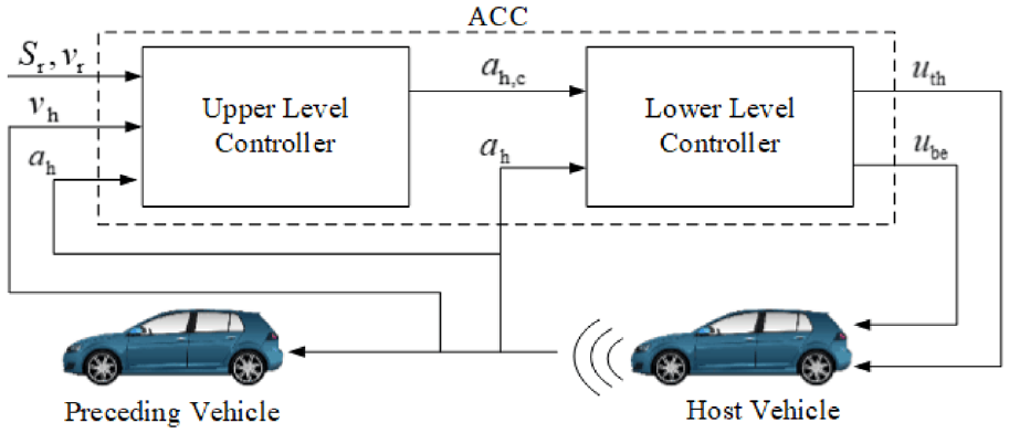
Hierarchical structure of the proposed ACC system.

When considering the throttle position and braking pressure signals transmitted to the host vehicle, time delays of responses of vehicle power train and braking systems are inevitable. In order to compensate the delays, first-order lag models are generally adopted in constructing the car-following dynamics of the host vehicle. The longitudinal dynamics of the host vehicle are then approximated as the following first-order lag model⁸

T_{1} d a_{h} (t) / d a_{h} (t) d t d t + a_{h} (t) = a_{h, c} (t)

(1)

where constant T₁ represents the first-order lag of actuators, a_h(t) is the acceleration of the host vehicle at time t ≥ 0 and a_{h, c}(t) is the acceleration command of the host vehicle.

For the controller in the upper layer, the tracking inter-vehicle distance error is defined as e(t) = s_r,_s(t) – s_r(t), where s_{r, s}(t) is the safe spacing. In general, the constant time headway strategy is employed to define the safe spacing

s_{r, s} (t) = T_{2} v_{h} (t) + s_{r, 0}

(2)

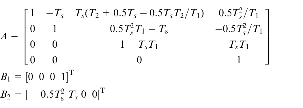
with the minimal safe inter-vehicle distance s_r,₀ > 0 and the time headway T₂ > 0. In the ACC system shown in Figure 1, the variable a_h,c(t) will be calculated real-time via PCC. Hence, the discrete-time version corresponding to the continuous-time model (1) is obtained using the zero-order holder with a sampling interval T_s. Then an incremental model is adopted to describe the dynamics of the ACC system as

x (k + 1) = Ax (k) + B_{1} Δ u (k) + B_{2} d (k)

(3)

where the state vector x(k) = (e(k), v_r(k), a_h(k), u(k-1))^T, control input u(k) = a_{h, c}, incremental control Δu(k) = u(k) – u(k – 1) and disturbance input d(k) = a_p(k) is the acceleration value of the preceding vehicle. The matrices are given as

\begin{matrix} A = [\begin{matrix} 1 & - T_{s} & T_{s} (T_{2} + 0.5 T_{s} - 0.5 T_{s} T_{2} / T_{1}) & 0.5 T_{s}^{2} / T_{1} \\ 0 & 1 & 0.5 T_{s}^{2} T_{1} - T_{s} & - 0.5 T_{s}^{2} / T_{1} \\ 0 & 0 & 1 - T_{s} T_{1} & T_{s} T_{1} \\ 0 & 0 & 0 & 1 \end{matrix}] \\ B_{1} = {[\begin{matrix} 0 & 0 & 0 & 1 \end{matrix}]}^{T} \\ B_{2} = {[\begin{matrix} - 0.5 T_{s}^{2} & T_{s} & 0 & 0 \end{matrix}]}^{T} \end{matrix}

(3)

Constraints and objectives

One of the basic functionalities of ACC is to regulate the host car to approach to its predecessor while maintaining a desired vehicle inter-vehicle distance, that is

objective (A) : e (k) \to 0, v_{r} (k) \to 0 as k \to \infty

(4)

where v_r(k) = v_p(k) – v_h(k). Then we consider the ride comfort performance of the ACC system. It is known that ride comfort is generally dominated by the vehicle acceleration in such a way that small amplitude of acceleration changes (i.e. jerk) can improve ride comfort. Hence, the changes in vehicular acceleration have to be minimized. To obtain the better ride comfort, one should minimize both the values of vehicular acceleration and jerk, that is

objective (B) : min {| a_{h} (k) |, | j_{h} (k) |}

(5)

where j_h(k) = Δu(k)/T_s. Note that the two objectives in equations (4) and (5) are conflicting since decreasing the acceleration and/or jerk can raise the comfort performance of the host vehicle but will degrade the car-following ability of ACC systems.

Due to the requirements of safe car-following and ride comfort, one should consider physical limits of vehicles. Namely, the ACC system is subject to constraints on the state and control variables given by

u_{\min} \leq u (k) \leq u_{\max}, Δ u_{\min} \leq Δ u (k) \leq Δ u_{\max}

(6)

where constants u_min, u_max, Δu_min and Δu_max are the minimal acceleration command, maximal acceleration command, minimum jerk and maximum jerk, respectively. In general, the bounds satisfy |u_min| > |u_max| and |Δu_min| > |Δu_max| due to the safety concern, that is, rear-end collisions avoidance. On the other hand, the spacing s_r(k) should not be more than the maximum safe spacing s_r,_max since a large inter-vehicle distance usually results in frequent vehicles’ cut-ins from adjacent lanes. Here let s_r,_max = T₂v_h,_max + s_r,₀ with a maximum speed v_h,_max of the host vehicle. For clarification, here the state constraints are formulated as the compacted form of

x (k) \in X, \forall k = 0, 1, \dots

(7)

with the box

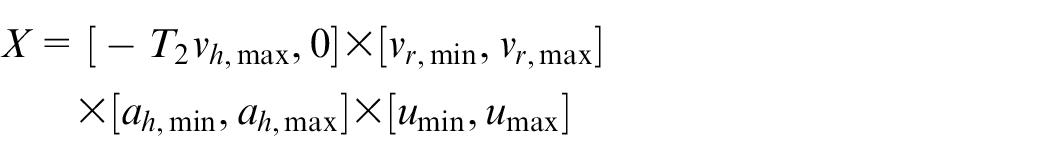
X = [- T_{2} v_{h, \max}, 0] \times [v_{r, \min}, v_{r, \max}] \times [a_{h, \min}, a_{h, \max}] \times [u_{\min}, u_{\max}]

where constants v_r,_max < 0, v_r,_max > 0, a_h,_min < 0 and a_h,_max > 0 are bounds satisfying that |a_h,_min| > |a_h,_max|.

In ACC, there exist multiple cruise objectives of vehicles, for example, safety, car-following and ride comfort. The primary objective of ACC is typically to track the preceding vehicle keeping the safe spacing s_r,s(k) for all times. In this paper, we use MPC to reconcile the conflicting objectives of ACC and then propose the new PCC algorithm to achieve the control goal.

PCC controller design

In this section, the PCC law computing the optimal acceleration commands is determined by solving a multi-objective MPC problem with varying weights in the receding horizon fashion. Considering the multiple objectives of ACC in equations (4) and (5), we adopt several stage cost criteria to represent the objectives of an ACC system. In terms of v_r(k) and e(k), a two-norm cost criterion is exploited to describe the car-following ability of the host car,⁴ that is

L_{1} (x (k)) = w_{e} x_{1}^{2} (k) + w_{v} x_{2}^{2} (k)

(8)

where weights w_e > 0 and w_v > 0. Note that a soft acceleration response will generally improve ride comfort and fuel economy of the host car, which is formulated by the following cost criterion

L_{2} (x (k)) = w_{a} x_{3}^{2} (k) + w_{ac} x_{4}^{2} (k)

(9)

where weights w_a > 0 and w_ac > 0. To limit frequent variation of the engine speed and to raise longitudinal ride comfort, the changes of acceleration commands (i.e. jerk) should be restrained. Hence, the cost criterion on Δu is used to describe this requirement, that is

L_{3} (u (k)) = w_{du} Δ u^{2} (k)

(10)

where weight w_du > 0. In order to make a trade-off among these costs, here we use some varying weights to sum them as a single cost function and the weights representing the relative importance of objectives are online determined according to real-time traffic scenarios.

Let an integer p > 0 be the prediction horizon. Then weighted finite horizon cost function of PCC is defined as

J (x, Δ u) = \sum_{i = 0}^{p - 1} {x^{T} (i | k) W (k) x (i | k) + w_{du} Δ u^{2} (i | k)}

(11)

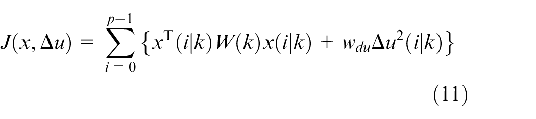
where weight matrix W(k) = diag{w_e(k), w_v(k), w_a(k), w_ac(k)}. In practical, driving behaviors of the preceding vehicle are changeable and often unpredicted. To accommodate this phenomenon, in Zhao et al.,³¹ some time-varying weights are recommended to be adopted to satisfy the complex driving behaviors of the preceding vehicle. Here the weights w_e(k), w_v(k) and w_a(k) are adjusted by Zhao et al.³¹

{\begin{matrix} w_{e} (k) = \frac{1 - N (s_{r} (k - 1))}{γ (k)} w_{e} (0) \\ w_{v} (k) = \frac{1 - N (v_{r} (k - 1))}{γ (k)} w_{v} (0) \\ w_{a} (k) = \frac{1 - N (s_{r} (k - 1)) \cdot N (v_{r} (k - 1))}{γ (k)} w_{a} (0) \end{matrix}

(12)

where

\begin{matrix} N (.) = \frac{2}{π} ta n^{- 1} (.) \\ γ (k) = [1 - N (s_{r} (k - 1))] w_{e} (0) + [1 - N (v_{r} (k - 1))] w_{v} (0) \\ + [1 - N (s_{r} (k - 1)) \cdot N (v_{r} (k - 1))] w_{a} (0) \end{matrix}

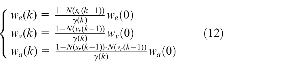
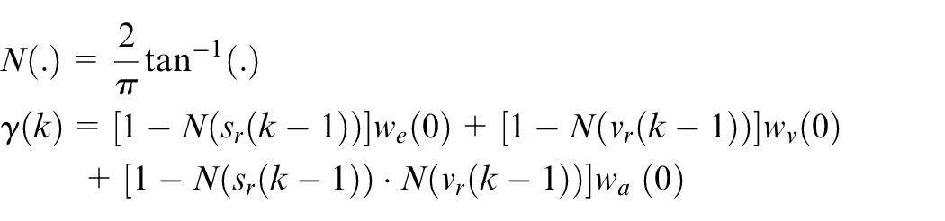
where w_e(0), w_v(0) and w_a(0) are initial values at time k = 0.

Remark 1

Similar to the available PCC algorithms, weights in the cost function (equation (11)) are not necessary to efficiently represent the requirements of the separate objective. For instance, increasing the value of w_du will be beneficial to smooth responses of the ACC system and then improve ride comfort of vehicles, but degrade the car-following ability. Moreover, selection of weights cannot efficiently attenuate high-frequency signals and peaks of the cruise commands. Note that from the standpoints of enlarging the working life of systems’ actuators and fuel saving, the control input of the system should not change frequently in a short time and its increments or decrements at one time should not be too large. Hence, it is necessary to ACC systems that high-frequency signals and peaks of the cruise commands of vehicles have to be attenuated in a systematic manner in order to raise the working life of vehicles and ride comfort.

Motivated by the idea of stair-like piecewise input, here we parameterize the predicted incremental acceleration commands as the geometric proportion function on the incremental acceleration command at the current time with a ratio of β. In terms of functionality, this parameterization of predicted variables can be viewed as a low-pass filter imposing the predicted variables. A schematic diagram of the stair-like control strategy is shown in Figure 2. In this way, the changes of predicted acceleration commands of ACC are along the same direction during a prediction process.

Figure 2.

Schematic diagram of the stair-like control strategy.

According to the idea of the stair-like control strategy, the incremental control actions of equation (3), Δu(i|k), over the prediction horizon [k, k + p] are planned as

Δ u (i | k) = β Δ u (i - 1 | k), i = 1, 2, . . ., p

which is equal to

Δ u (i | k) = β^{i} Δ u (0 | k), i = 1, 2, \dots, p

(13)

where constant 0 < β < 1 is the stair factor and Δu(i|k) is the future value of incremental control action at time k + i predicted at the current time k. An immediate benefit of the stair-like control strategy is that the size of the PCC optimization is reduced significantly since the p control actions to be computed in PCC are explicit functions on the current action. It is clear that the predicted control actions will approach to a constant when the window p is long enough. Moreover, a larger β leads to softer profiles of velocity and acceleration of the host vehicle,⁹ which improves ride comfort of vehicles. Hence, one can directly adjust β to guarantee ride comfort of vehicles from the viewpoints of design of ACC strategies.

Considering the ACC system (equation (3)) with the stair-like control actions (equation (13)), we have the predicted state evaluations over the prediction window p, that is

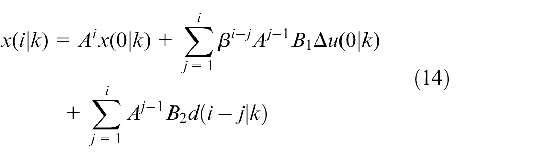
\begin{matrix} x (i | k) = A^{i} x (0 | k) + \sum_{j = 1}^{i} β^{i - j} A^{j - 1} B_{1} Δ u (0 | k) \\ + \sum_{j = 1}^{i} A^{j - 1} B_{2} d (i - j | k) \end{matrix}

(14)

where i = 1, 2,…, p. Since the predecessor’s acceleration over the window p is unknown, here we exploit its estimate at the previous times to approximate the future terms. Let d(k – 1) = d(p – j|k), j = 1, 2,…, p. Then we have the compact form of the future state evaluations of equation (3)

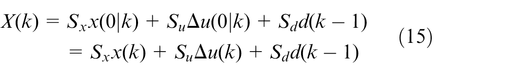
\begin{array}{l} X (k) = S_{x} x (0 | k) + S_{u} Δ u (0 | k) + S_{d} d (k - 1) \\ = S_{x} x (k) + S_{u} Δ u (k) + S_{d} d (k - 1) \end{array}

(15)

where x(0|k) = x(k) is the state at the current time k, X(k) = (x^T(1|k), x^T(2|k),…, x^T(p|k))^T and matrices

S_{u} = [\begin{matrix} B_{1} \\ β A B_{1} \\ ⋮ \\ \sum_{i = 1}^{p} β^{p - i} A^{i - 1} B_{1} \end{matrix}]

S_{d} = [\begin{matrix} B_{2} \\ A B_{2} \\ ⋮ \\ \sum_{i = 1}^{p} A^{i - 1} B_{2} \end{matrix}]

S_{x} = [\begin{matrix} A \\ A^{2} \\ ⋮ \\ A^{p} \end{matrix}]

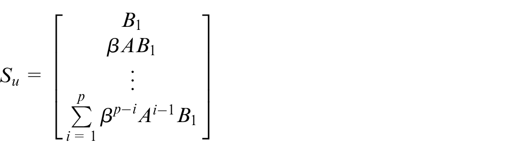
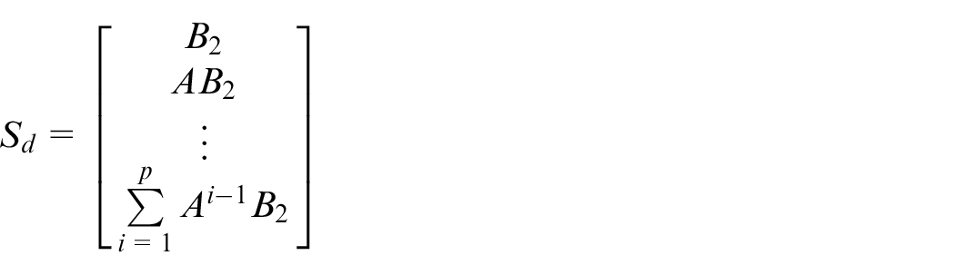
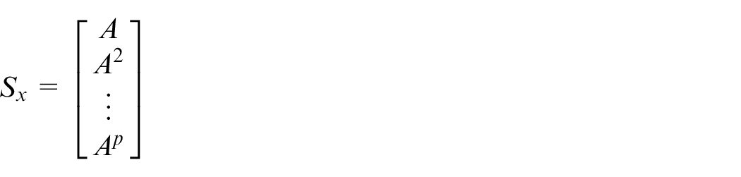
Moreover, considering the constraints (7) and (13), we have

Δ {\bar{u}}_{min} (k) \leq Δ u (k) \leq Δ {\bar{u}}_{max} (k) \infty

(16)

with bounds

\begin{matrix} Δ {\bar{u}}_{\min} (k) = \max {Δ u_{\min}, \frac{u_{\max} - u (k - 1)}{\sum_{i = 0}^{p - 1} β^{i}}} \\ Δ {\bar{u}}_{\max} (k) = \min {Δ u_{\max}, \frac{u_{\min} - u (k - 1)}{\sum_{i = 0}^{p - 1} β^{i}}} \end{matrix}

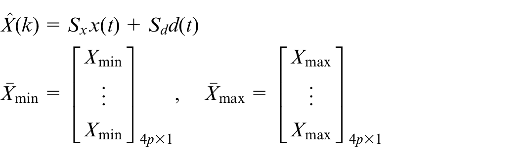
Now we consider the state constraints in equation (7). Let X_min = [–T₂v_h,_max, v_r,_min, a_h,_min, u_min]^T and X_max = [0, v_r,_max, a_h,_max, u_min]^T. From equation (14), it is obtained that

{\bar{X}}_{min} (k) - \hat{X} (k) \leq S_{u} Δ u (k) \leq {\bar{X}}_{max} (k) - \hat{X} (k)

(17)

with

\begin{matrix} \hat{X} (k) = S_{x} x (t) + S_{d} d (t) \\ {\bar{X}}_{min} = {[\begin{matrix} X_{min} \\ ⋮ \\ X_{min} \end{matrix}]}_{4 p \times 1}, {\bar{X}}_{max} = {[\begin{matrix} X_{max} \\ ⋮ \\ X_{max} \end{matrix}]}_{4 p \times 1} \end{matrix}

Substituting equations (13)–(14) into the cost function (equation (11)), it is obtained that

\begin{matrix} J (x (k), Δ u (k)) = X^{T} (k) \hat{W} X (k) + R Δ u^{2} (k) \\ = {\hat{X}}^{T} (k) \hat{W} \hat{X} (k) + 2 {\hat{X}}^{T} (k) \hat{W} S_{u} Δ u (k) \\ + (S_{u}^{T} {\hat{W}}_{x} S_{u} + R) Δ u^{2} (k) \end{matrix}

(18)

where $\hat{W} (k) = diag {W (k), \dots, W (k)}$ and R = w_du(1 + β + ··· + β^p – 1). At each sampling time k, the PCC controller is determined by solving the following finite-horizon optimal control problem

\begin{matrix} \min_{Δ u (k)} J (x (k), Δ u (k)) \\ s . t . {\bar{X}}_{min} (k) - \hat{X} (k) \leq S_{u} Δ u (k) \leq {\bar{X}}_{max} (k) - \hat{X} (k) \\ Δ {\bar{u}}_{\min} \leq Δ u (k) \leq Δ {\bar{u}}_{max} \\ x (0 | k) = x (k) \end{matrix}

(19)

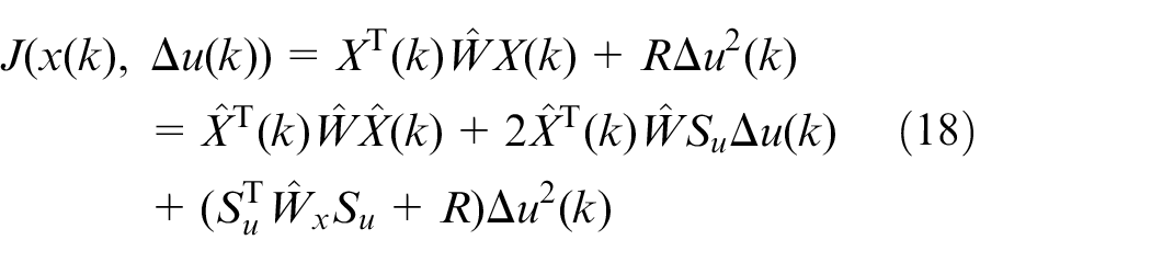
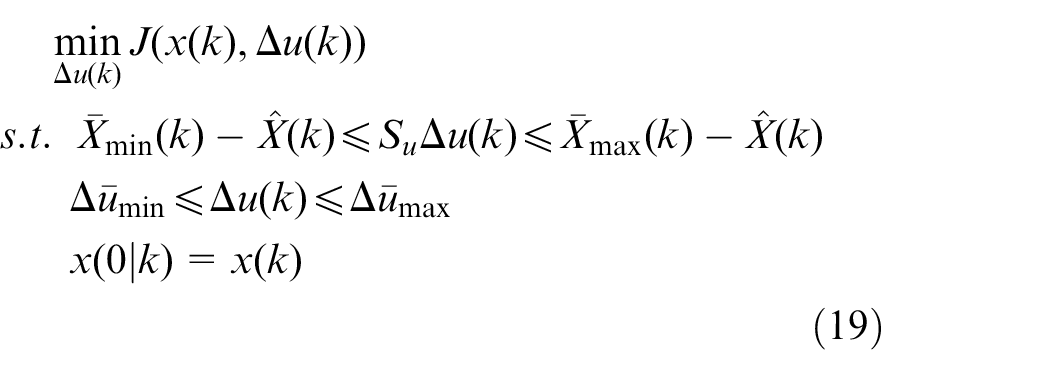
where x(k) is the state measurement at time k. When the constraints in equation (19) are assumed to be omitted, we have the optimal solution by Lagrange’ optimization method

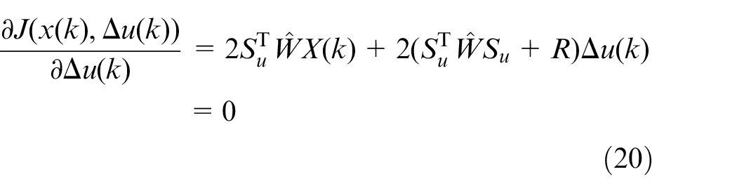
\begin{matrix} \frac{\partial J (x (k), Δ u (k))}{\partial Δ u (k)} = 2 S_{u}^{T} \hat{W} X (k) + 2 (S_{u}^{T} \hat{W} S_{u} + R) Δ u (k) \\ = 0 \end{matrix}

(20)

Then it is derived that

Δ u^{*} (k) = - \frac{S_{u}^{T} \hat{W} X (k)}{S_{u}^{T} \hat{W} S_{u} + R}

(21)

Obviously, the optimal incremental control equation (21) is not necessarily to satisfy the constraints in equation (19). To this end, a numerical programming solver should be adopted to solve the optimization problem with the constraints. Denote Δu^*(k) by the corresponding optimal solution to equation (19). Then, the obtained PCC controller is determined as

u^{pcc} (k) = u (k - 1) + Δ u^{*} (k), \forall k = 1, 2, \dots

(22)

Remark 2

Note that due to the stair-like control strategy, the decision variables of the PCC optimization problem defined in equation (19) are reduced to only one decision variable. Therefore, any efficient numerical programming algorithm can be used as one-dimensional search methods, such as Fibonacci method, golden section method.

In what follows, the proposed efficient PCC algorithm is summarized as follows:

Step 1 (initialization). Input the PCC parameters T_s > 0, p ≥ 1 and 0 < β < 1 and off-line compute matrices S_u, S_x and S_d; let k = 0 and d(–1) = 0.

Step 2. At time k, measure the current state x(k) and estimate the acceleration of the preceding vehicle, d(k – 1).

Step 3. Solve problem (19) with x(k) by the following steps:

3.1. Use s_r(k) and v_r(k) from x(k) to update $\hat{W}$ by equation (12) for the prediction horizon (0, p – 1).

3.2. Update the constraints in equations (16) and (17) and solve equation (19) by the quadratic programming solver.

3.3. Apply Δu^*(k) to the ACC system (equation (3)).

Step 4. Let k = k + 1, and return to Step 2.

Numerical simulations

In this section, three basic and classical scenarios are used to verify the effectiveness of the proposed PCC algorithm. In the first scenario, a preceding vehicle starts with a constant acceleration and then drives at a constant speed; in the second, a preceding vehicle normally accelerates and brakes; in the third, a preceding vehicle quickly accelerates and brakes. The actual traffic scenarios are often combinations of these basic scenarios. In this study, three PCC algorithms are compared to evaluate their performances, that is, traditional PCC algorithm³ (denoted as T-PCC), the stair-like PCC algorithm with constant weights (denoted as constants weights predictive cruise control (CS-PCC)) and the stair-like PCC algorithm with varying weights (denoted as varying weights predictive cruise control (VS-PCC)). The parameters of the ACC system are listed in Table 1.

Table 1.

Parameters of the ACC system.

Symbol	Description	Values
T_s	Sampling time	0.2 s
T ₁	Time constant	0.5 s
T ₂	Desired time headway	0.2 s
S_r,s	Safely tracking distance	2 m
v _min, v_max	Minimal, maximal velocity	0 m/s, 30 m/s
β	Tuning number	0.7
a _min, a_max	Minimal, maximal acceleration	−5.5 m/s², 2.5 m/s²
u _min, u_max	Minimal, maximal command	−5.5 m/s², 2.5 m/s²
Δu_min, Δu_max	Minimal, maximal control	–2 m/s², 2 m/s²
j _min, j_max	Minimal, maximal jerk	−2 m/s³, 2 m/s³
w_e	Headway error initial value	1
w_v	Relative velocity initial value	1
w_a	Acceleration weight initial value	10
w_ac	Command weight initial value	5

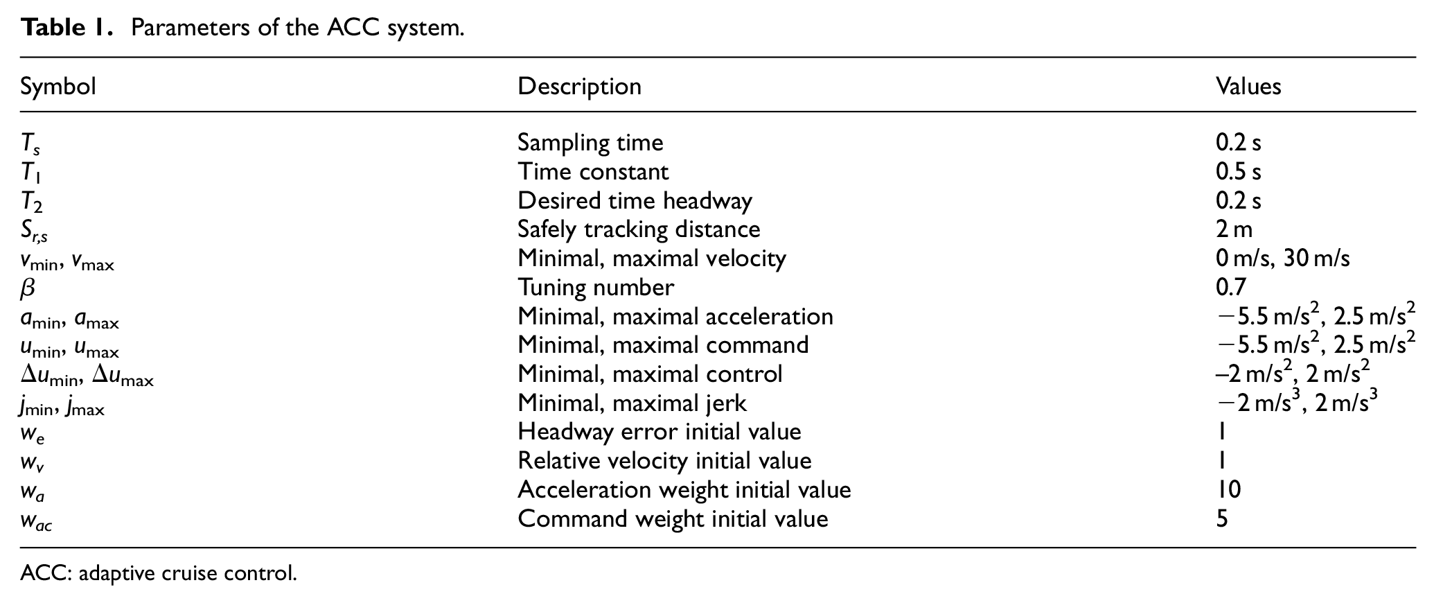
ACC: adaptive cruise control.

Scenario 1: accelerating and driving with constant speed

In this scenario, the green light comes before the preceding vehicle started. It is assumed that the preceding vehicle is accelerated with 2.5 m/s² and then driven at a constant speed of v_p = 20 m/s (see Figure 3(a)). Figure 3(b)–(f) shows the time evolutions of inter-vehicle distance, acceleration, control command, car-following errors and jerk of the host vehicle obtained by separately applying T-PCC (blue dotted lines), CS-PCC (red solid lines) and VS-PCC (green dash-dotted lines). In order to prevent the vehicle’s cut-ins from adjacent lanes, the fast response of ACC is required to make the host vehicle start rapidly and the acceleration command curve will be calculated by the ACC upper controller. Then the lower controller makes the host vehicle track the acceleration command by regulating the throttle and brake pedal, the host vehicle equipped with three algorithms could reach the speed of preceding vehicle, of which error to preceding vehicle’s velocity is 0.06, 0.00 and 0.04 m/s, respectively, as shown in Figure 3(a). It can be observed for Figure 3(b) that the three PCC algorithms can keep the safe inter-vehicle distance to avoid collision, but the VS-MPC algorithm outperforms both of the T-PCC and CS-PCC algorithms in terms of tracking the preceding vehicle.

Figure 3.

Simulation results of T-PCC, CS-PCC and VS-PCC in Scenario 1: (a) velocity of the preceding car, (b) inter-vehicle distance, (c) car’s acceleration, (d) acceleration command, (e) acceleration error and (f) car’s jerk.

On the other hand, one can see from Figure 3(e) that compared to the T-PCC algorithm, the CS-PCC algorithm has less tracking error in acceleration command and reduces the peak of acceleration and jerk of the host vehicle in Figure 3(f). This leads to the smoother responses of velocity or acceleration/deceleration command of the host vehicle (see Figure 3(d)). Moreover, the VS-PCC algorithm outperforms a little the CS-PCC algorithm in terms of tracking errors and jerk, as shown in Figure 3(e)–(f). Hence, the car-following ability and ride comfort can be improved obviously by the proposed PCC algorithms.

Scenario 2: preceding vehicle encountered a pedestrian

In this scenario, the preceding vehicle is assumed to be driven at speed v_p = 15 m/s and then taken an emergence braking to decelerate when a pedestrian appears in front of the preceding vehicle at 12 s. The preceding vehicle is kept to be driven at v_p = 4 m/s (see Figure 4(a)). Figure 4(b)–(f) shows the time evolutions of the inter-vehicle distance, acceleration, control command, tracking error in acceleration command and jerk of the host vehicle obtained by applying the T-PCC algorithm (blue dotted lines), CS-PCC (red solid lines) algorithm and VS-PCC algorithm (green dash-dotted lines), respectively. In order to avoid rear-collision due to emergency braking, the fast response of ACC is required to make host vehicle to take an emergence braking at 12 s. As shown in Figure 4(b)–(f), three algorithms can all guarantee the safe inter-space, but CS-PCC and VS-PCC have relatively large inter-vehicle distances in order to avoid collision and ensure the driving safety.

Figure 4.

Simulation results of T-PCC, CS-PCC and VS-PCC in Scenario 2: (a) velocity of the preceding car, (b) inter-vehicle distance, (c) car’s acceleration, (d) acceleration command, (e) acceleration error and (f) car’s jerk.

Before the preceding vehicle quickly brakes, the host vehicle controlled by CS-PCC or VS-PCC has a smoother jerk profile to provide the more comfortable ride. When the preceding vehicle quickly brakes, the host vehicle has larger deceleration to avoid collision by ignoring the ride comfort as safety is the primary concern. As shown in Figure 4(d), the acceleration profiles of CS-PCC and VS-PCC have smaller fluctuations, and meanwhile, CS-PCC and VS-PCC performed better than T-PCC in tracking errors in acceleration command, as shown in Figure 4(e). The amplitudes of jerk of CS-PCC and VS-PCC are smaller than that of T-PCC, as shown in Figure 4(f). This implies that passengers feel more comfort than vehicles by T-PCC. At the same time, the smaller change of the accelerations can effectively reduce fuel consumption. Finally, the three PCC algorithms make the host vehicle to track the preceding with the similar speed and the error to the preceding vehicle’s velocity is 0.025, 0.388 and 0.248 m/s, respectively, which are within the scope permitted.

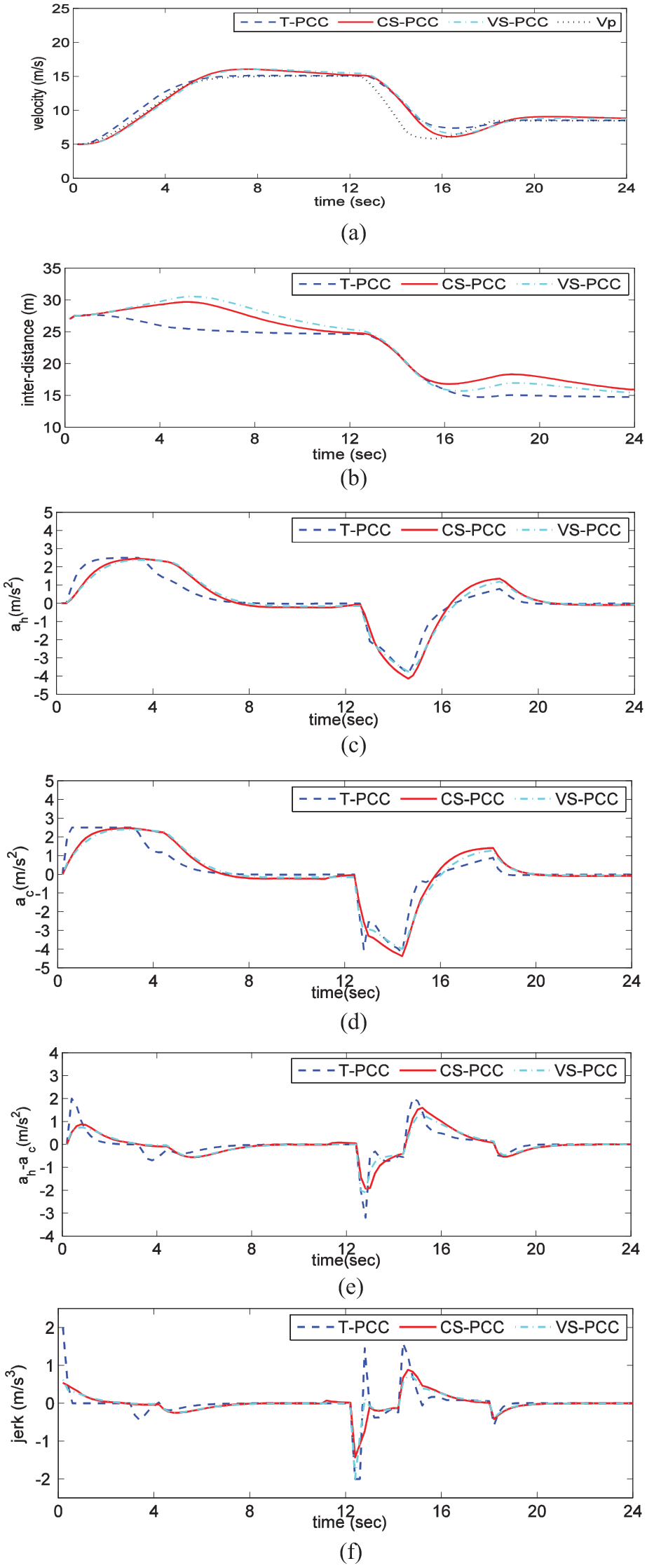
Scenario 3: rapid acceleration and deceleration

In this scenario, the preceding vehicle is accelerating to try to go across an intersection before the green light is turned off. Hence, it is possible to take an emergency deceleration due to the deficiency of time. The preceding vehicle accelerates from 0 m/s to v_p = 10 m/s and keeps driving at this speed. At time 12 s, the green light is over and the preceding vehicle fails to reach the intersection and has to make an emergency stop. The speed profile of the preceding vehicle is pictured as the black dotted line in Figure 5(a). Figure 5(a)–(f) shows the time evolutions of velocity, inter-vehicle distance, acceleration, control command, tracking error in acceleration command and jerk of the host car obtained by separately applying T-PCC (blue dotted lines), CS-PCC (red solid lines) and VS-PCC (green dash-dotted lines). From Figure 5(b), one can see that three approaches satisfy tracking ability and keep the host vehicle driving at velocity v_h = 15 m/s as soon as possible as shown in Figure 5(a), besides, all three algorithms’ tracking errors to preceding vehicle’s velocity are 0.587, 0.318 and 0.147 m/s, but VS-PCC has the larger inter-vehicle distance. From Figure 5(c)–(e), one can see that the acceleration of the host vehicle can track the acceleration command profile, but the curve tracking ability of CS-PCC and VS-PCC is the highest as shown in Figure 5(e). In addition, it can be seen from Figure 5(f) that the jerk peak by T-PCC gets to 2 m/s², which is more than that by CS-PCC and VS-PCC. Both CS-PCC and VS-PCC reduce dramatically jerk peak of the host vehicle, with improvement of 51.16% and 23.07%, respectively, compared to T-PCC. Therefore, the proposed PCC algorithm could ensure the safety and car-following ability while improving ride comfort.

Figure 5.

Simulation results of T-PCC, CS-PCC and VS-PCC in Scenario 3: (a) velocity of the preceding car, (b) inter-vehicle distance, (c) car’s acceleration, (d) acceleration command, (e) acceleration error and (f) car’s jerk.

Further discussions

In the proposed PCC algorithm, the decision variables over the prediction horizon are parameterized by the control action at the current time. Hence, the number of decision variables is merely determined by the number of control variable. This implies that the computational load of online solving the PCC optimization problem will be decreased considerably.³²,³⁵ It can be seen from Figure 6 –8 that the computing times at each time of CS-PCC and VS-PCC are shorter than that of T-PCC significantly. Table 2 lists that the average calculating times at one time of the three PCC algorithms, where the CS-PCC algorithm outperforms the T-PCC algorithm with improvements of 77.40%, 46.06% and 69.25% in the aforementioned three scenarios, respectively. Similarly, the VS-MPC algorithm improves 79.09%, 48.80% and 70.61% compared to the T-PCC algorithm in the aforementioned three scenarios, respectively. Thus, the proposed PCC algorithm saves the computing time required significantly.

Figure 6.

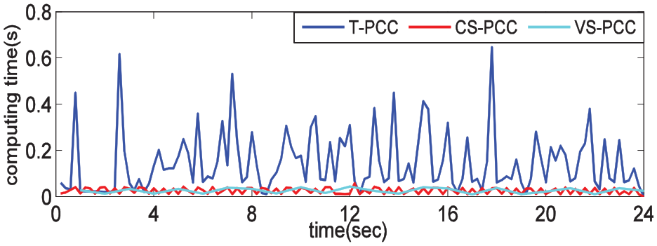
Computing times at one time in scenario 1.

Figure 7.

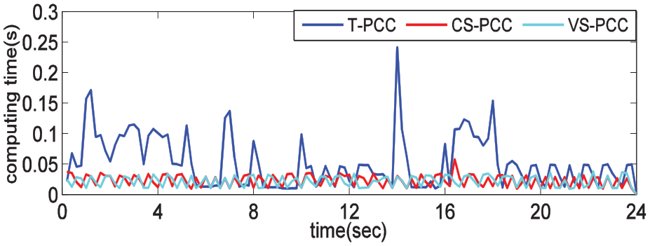
Computing times at one time in scenario 2.

Figure 8.

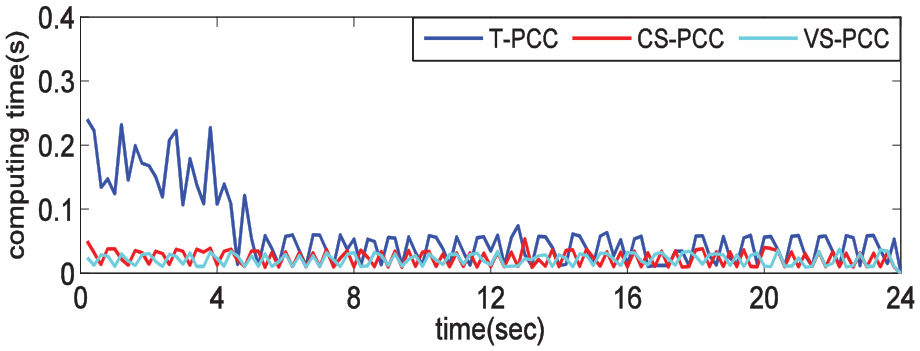
Computing times at one time in scenario 3.

Table 2.

Average computing time at one time in three scenarios.

Cases	Computing time (ms)			Improvement
Cases	T-PCC	CS-PCC	VS-MPC
Case 1	110.5546	24.9832	23.1190	77.40%	79.09%
Case 2	43.8319	23.6429	22.4412	46.06%	48.80%
Case 3	78.3193	24.0840	23.0174	69.25%	70.61%

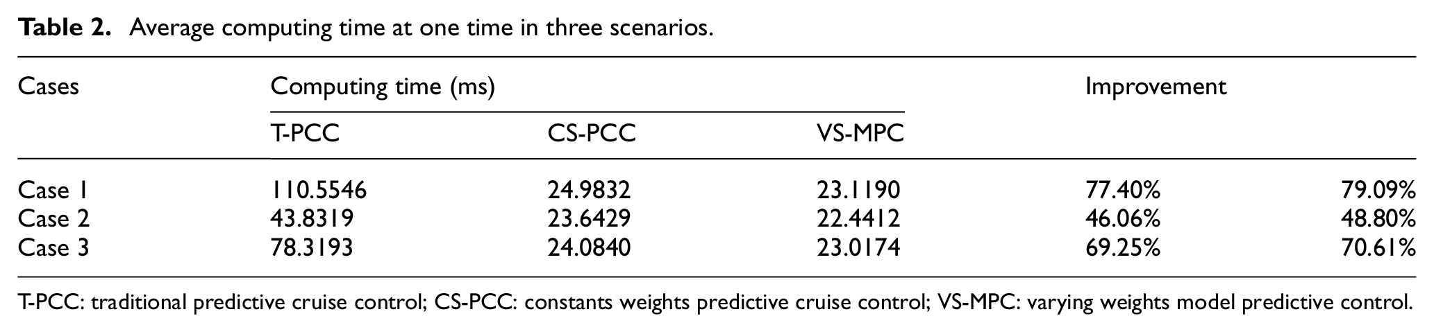
T-PCC: traditional predictive cruise control; CS-PCC: constants weights predictive cruise control; VS-MPC: varying weights model predictive control.

Now we further compare the peaks of the jerk profiles obtained by the three PCC algorithms. Table 3 lists the peaks by the three PCC algorithms in the aforementioned three scenarios and Figure 9 shows their variances of the jerk profiles. From Table 3, one can see that the CS-PCC and VS-PCC algorithms can attenuate the peaks of jerk more efficiently than the T-PCC algorithm by decreases of 65.6%, 30.0% and 0% and by 74.25%, 0% and 69.20%, respectively. Moreover, it is observed from Figure 9 that the variances of the jerk profiles obtained by the CS-PCC and VS-PCC algorithms are smaller than that by the T-PCC algorithm. These imply that the ACC system equipped with the proposed PCC algorithms gain smoother acceleration responses and more comfortable ride experiences. In addition, VS-PCC algorithm outperforms a little the CS-PCC algorithm in terms of acceleration and jerk. The reason is that the weights of the cost function in VS-PCC can be self-adjusted to response to the changes of its preceding vehicles’ driving behaviors. In this sense, the VS-PCC algorithm has ability to adapt more complex and changeable traffic scenarios than the CS-PCC algorithm.

Table 3.

Peak of jerk in three scenarios.

Cases	Peak of jerk (m/s³)			Improvement
	T-PCC	CS-PCC	VS-PCC
Case 1	2.0	0.688	0.515	65.6%	74.25%
Case 2	2.0	1.40	2.0	30.0%	0
Case 3	2.0	2.0	0.616	0	69.20%

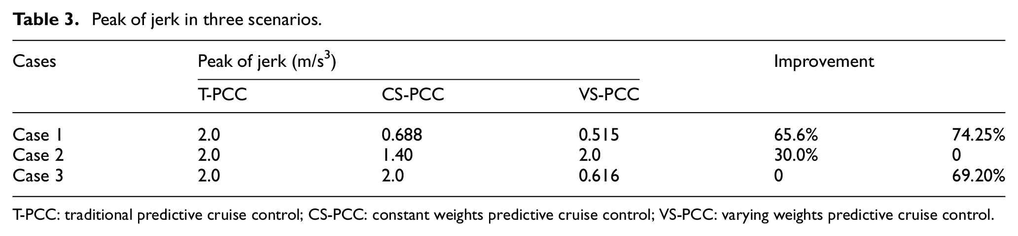
T-PCC: traditional predictive cruise control; CS-PCC: constant weights predictive cruise control; VS-PCC: varying weights predictive cruise control.

Figure 9.

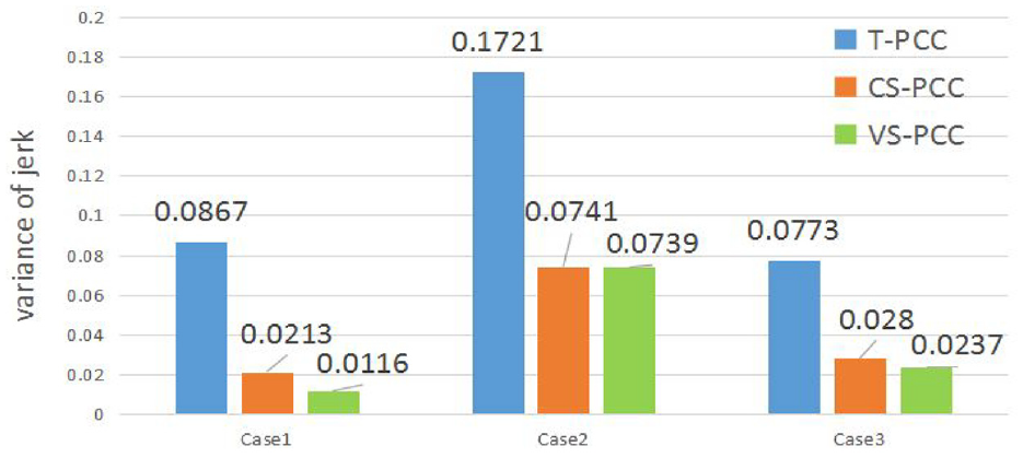
Variances of jerk in three scenarios.

Conclusion

In this paper, we proposed a novel PCC algorithm with slight computational burden for vehicular ACC systems. The changes of the planned command profile of the PCC were pre-planned to be along the same direction within the prediction horizon and the weights of its cost function were self-adjusted to response to changes of the preceding vehicles’ driving behaviors. The advantage of the new PCC algorithm is its ability to smooth the acceleration profiles and responses of the ACC system and reduce the online computational load of the PCC controller. As a result, the ride comfort, car-following capability and safety of vehicles can be efficiently satisfied in the proposed PCC controller. Some comparison results on three representative traffic scenarios demonstrated the proposed PCC approach and evaluated its effectiveness in terms of ride comfort, car-following capability and computational demand.

Footnotes

Declaration of conflicting interests

The author(s) declared no potential conflicts of interest with respect to the research, authorship and/or publication of this article.

Funding

The author(s) disclosed receipt of the following financial support for the research, authorship and/or publication of this article: The work was supported by the National Natural Science Foundation of China (Nos 61773345 and 61803336), Zhejiang Provincial Natural Science Foundation of China (No. LR17F030004) and Foundation of State Key Laboratory of Automotive Simulation and Control (No. 20171103).

ORCID iDs

Defeng He

Xiulan Song

References

Marsden

McDonald

Brackstone

. Towards an understanding of adaptive cruise control. Transport Res C-Emer 2001; 9(1): 33–51.

Plessen

Bernardini

Esen

, et al. Spatial-based predictive control and geometric corridor planning for adaptive cruise control coupled with obstacle avoidance. IEEE T Contr Syst T 2017; 26(1): 38–50.

Luo

Liu

, et al. Model predictive control for adaptive cruise control with multi-objectives: comfort, fuel- economy, safety and car-following. J Zhejiang Univ-Sc A 2010; 11(3): 191–201.

Lin

Hsu

Chen

, et al. Dynamic programming for model predictive control of adaptive cruise control systems. In: IEEE international conference on vehicular electronics and safety, Yokohama, Japan, 5–7 November 2016, pp. 202–207. New York: IEEE.

Zhang

Ioannou

. Longitudinal control of heavy trucks in mixed traffic: environmental and fuel economy considerations. IEEE T Intell Transp 2006; 7(1): 92–104.

Ganji

Kouzani

Khoo

, et al. Adaptive cruise control of a HEV using sliding mode control. Expert Syst Appl 2014; 41(1): 607–615.

Mohammadreza

Jalali

Mashhadi

SKM

. Robust adaptive cruise control of high speed trains. ISA T 2014; 52(2): 533–541.

Rajamani

, et al. Model predictive multi-objective vehicular adaptive cruise control. IEEE T Contr Syst T 2011; 19(3): 556–566.

Wang

Zhao

Zhang

, et al. Multi-model fuzzy controller for vehicle lane tracking. In: IEEE international conference on intelligent transportation systems, Qingdao, China, 8–11 October 2014, pp. 1341–1346. New York: IEEE.

10.

Naus

Ploeg

Molengraft

. Design and implementation of parameterized adaptive cruise control: An explicit model predictive control approach. Control Eng Pract 2010; 18(8): 882–892.

11.

Ahmed

Svaricek

. Adaptive robust gain scheduled control of vehicle semi-active suspension for improved ride comfort and road handling. In: IEEE international conference on mechatronics, Vicenza, Italy, 27 February–1 March 2013, pp. 376–381. New York: IEEE.

12.

Kim

Tomizuka

Cheng

. Smooth motion control of the adaptive cruise control system by a virtual lead vehicle. Int J Automot Techn 2012; 13(1): 77–85.

13.

Wang

, et al. Economy-oriented vehicle adaptive cruise control with coordinating multiple objectives function. Vehicle Sys Dyn 2013; 51(1): 1–17.

14.

Rawlings

Mayne

. Model predictive control: theory and design. Nob Hill Publishing, LLC, 2009. Madison, WI, USA.

15.

Wang

Sun

. On stability of multiobjective NMPC with objective prioritization. Automatica 2015; 57: 189–198.

16.

Hou

Sun

Hofmann

. Adaptive model predictive control with propulsion load estimation and prediction for all-electric ship energy management. Energy 2018; 150: 877–889.

17.

Qiu

Lou

. Fuel efficiency-oriented platooning control of connected nonlinear vehicles: a distributed economic MPC approach. Asian J Control. Epub ahead of print 18 February 2019. DOI: 10.1002/asjc.2049.

18.

Guo

Cao

Chen

, et al. Model predictive path following control for autonomous cars considering a measurable disturbance: implementation, testing, and verification. Mech Syst Signal Pr 2019; 118: 41–60.

19.

Chen

Wang

, et al. Nonlinear model predictive controller design based on learning model for turbocharged gasoline engine of passenger vehicle. Mech Syst Signal Pr 2018; 109: 74–88.

20.

Hou

Song

Park

, et al. Implementation and evaluation of real-time model predictive control for load fluctuations mitigation in all-electric ship propulsion systems. Appl Energ 2018; 230: 62–77.

21.

Sancar

FEBF

Huissoon

. MPC based collaborative adaptive cruise control with rear end collision avoidance intelligent vehicles symposium proceedings. In: IEEE intelligent vehicles symposium proceedings, Dearborn, MI, 8–11 June 2014, pp. 516–521. New York: IEEE.

22.

Sina

Wahde

. Fuel consumption optimization of heavy-duty vehicles using genetic algorithms. In: Proceedings of 2017 IEEE Congress on evolutionary computation, San Sebastian, 5–8 June 2017, pp. 29–36. New York: IEEE.

23.

Bijan

Vajedi

Azad

. Ecological adaptive cruise control of a plug-in hybrid electric vehicle for urban driving. In: International conference on intelligent transportation systems, Rio de Janeiro. Brazil, 1–4 November 2016, pp. 1739–1744. New York: IEEE.

24.

Shi

, et al. Multi-objective predictive cruise control for connected vehicle systems on urban conditions with InPA-SQP algorithm. Optim Contr Appl Met 2019; 40(3): 479–498.

25.

Moser

Schmied

Waschl

. Flexible spacing adaptive cruise control using stochastic model predictive control. IEEE T Contr Syst T 2018; 26(1): 114–127.

26.

Liu

. Reinforcement learning optimization look-ahead energy management of a parallel hybrid electric vehicle. IEEE T Mechatron 2017; 22(4): 1497–1507.

27.

Shakouri

Ordys

Askari

. Adaptive cruise control with stop & go function using the state-dependent nonlinear model predictive control approach. ISA T 2012; 51(5): 622–631.

28.

Kohut

Borrelli

Hedrick

, et al. PCC voltage analysis of a hybrid generating system in case of utility side fault. In: IEEE vehicle power and propulsion conference (VPPC), Seoul, South Korea, 9–12 October 2012.

29.

Lin

Nguyen

HLT

Wang

. Adaptive neuro-fuzzy predictive control for design of adaptive cruise control system. In: International conference on networking, sensing and control, Calabria, 16–18 May 2017.

30.

Hellström

Ivarsson

Aslund

, et al. Look-ahead control for heavy trucks to minimize trip time and fuel consumption. Control Eng Pract 2009; 17(2): 245–254.

31.

Zhao

Wong

Xie

, et al. Real-time weighted multi-objective model predictive controller for adaptive control system. Int J Automot Techn 2017; 18(2): 279–292.

32.

Chen

. Linear system theory and design. 3rd ed. Oxford: Oxford University Press, 1984.

33.

Cannon

. Efficient nonlinear model predictive control algorithms. Annu Rev Control 2004; 28(2): 229–237.

34.

Feng

. Risk Assessment and control for accounting information system based on fuzzy analytic hierarchy process. In: Proceedings of 8th international conference on measuring technology and mechatronics automation, Macau, China, 11–12 March, pp. 580–583. New York: IEEE.

35.

Naus

GJL

Ploeg

van de Molengraft

WPMH

, et al. A model predictive control approach to design a parameterized adaptive cruise control. Control Eng Pract 2010; 18(8): 882–892.