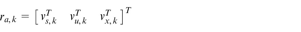
Fault estimation for a class of nonlinear time-variant systems through a Krein space

Abstract

This paper studies the $H_{\infty}$ fault estimation problem for a class of discrete-time nonlinear systems subject to time-variant coefficient matrices, online available input, and exogenous disturbances. By assuming that the concerned nonlinearity is continuously differentiable and by using Taylor series expansions, the dynamic system is transferred as a linear time-variant system with modeling uncertainties. A non-conservative but nominal system and its corresponding $H_{\infty}$ indefinite quadratic performance function are, respectively, given in place of the transferred uncertain system and the conventional performance metric, such that the estimation problem is converted as a two-stage optimization issue. By introducing an auxiliary model in Krein space, the so-called orthogonal projection technique is utilized to search an appropriate choice serving as the estimation of the fault signal. A necessary and sufficient condition on the existence of the fault estimator is given, and a recursive algorithm for computing the gain matrix of the estimator is proposed. The addressed method is applied to an indoor robot localization system to show its effectiveness.

Keywords

Fault estimation nonlinearity time-variant system Krein space uncertainty

Introduction

When sketching the works on model-based fault diagnosis (including fault detection, fault isolation, and fault estimation) from 1970s of the last century, different kinds of optimization techniques for robust control have been widely used in this area, which lead to the so-called robust fault diagnosis, for example, see previous works^1–6 and the references therein. The core idea behind model-based robust fault diagnosis is to construct a residual signal that prominently indicates whether a fault occurs in the system, but simultaneously reduces the effects from modeling uncertainties and exogenous disturbances/unknown inputs to this signal. Roughly speaking, by distinguishing the characteristics of the exogenous disturbance, existing contributions can be categorized into two types: that is, $H_{2}$ - and $H_{\infty}$ -based results. Compared to the $H_{2}$ -based results, the $H_{\infty}$ -based works do not require any prior knowledge on disturbance, which are more applicable when the unknown inputs are described as bounded signals rather than white noise sequences.^2,4

Until now, by using the $H_{\infty}$ optimization approaches, much efforts have been paid on fault diagnosis for linear systems with constant coefficient parameter matrices, namely, linear time-invariant (LTI) systems or different kinds of linear parameter-varying systems (which include switched systems and Markovian jump system), where for each mode, the dynamic model reduces to LTI system.^7–9 In recent years, in contrast with the progress of the aforementioned systems, some works on linear time-variant (LTV) systems appear, especially for linear discrete time-variant (LDTV) systems, which result from the fact that most of the real-world applications or industrial processes are intrinsically time-variant. Moreover, special efforts are required for time-variant systems since majorities of the existing results for systems with constant coefficient parameter matrices cannot be directly extended to time-variant cases, where the related performance indices, the optimization techniques, and online available algorithms are supposed to be newly proposed. We refer to previous works^4–6,10,11 for some representative results on this area.

Nonlinearity is also one of the inherent characteristics for practical systems, and therefore, researchers have devoted much to fault diagnosis for nonlinear systems with bounded inputs. In this literature, with the aid of mature results on fault diagnosis for LTI systems, there are lots of results on systems with nonlinear perturbations, where these systems can be viewed as special LTI systems with nonlinear disturbances.^4,12–14 In this manner, designer can extend results for LTI systems to those systems using offline $H_{\infty}$ optimization methods. Other results can be found in previous works^15–17 for different kinds of nonlinear systems, but one cannot find a unified approach for nonlinear systems. Apart from the existing results, fault diagnosis on nonlinear systems with time-variant coefficient matrices gradually gained attention.^18–24 The main obstacle for achieving successful fault diagnosis for this kind of systems lies in that, how to find a feasible way such that not only the nonlinearity can be reasonably tackled but also provide a cost-efficient algorithm for online implementation subject to time-varying coefficients.

In this study, we aim to propose a novel $H_{\infty}$ fault estimation method for a class of nonlinear time-variant systems, where the shape and amplitude of the fault are provided (compared to the results on fault detection that only deliver an alarm when the malfunction occurs). The nonlinearity is assumed to be continuously differentiable rather than in the form of state-dependent perturbations,^{18–20,22,23} and a dynamic filter acting as the fault estimator is designed through linear estimation methodology in Krein space. The contributions of the current study are three-folds:

A non-conservatism framework for estimating the fault is addressed after linearizing the nonlinear system.

A sufficient and necessary condition for the existence of the fault estimator is established.

A recursive algorithm for calculating the gain matrix of the estimator is given.

Notations

Throughout this study, $R^{n}$ describes the n-dimensional vector space. $0$ and $I$ , respectively, represent zero and identity matrix with appropriate dimensions. For a positive integer $N$ , $‖ ρ_{k} ‖_{2} = \sqrt{Σ_{k = 0}^{N} ρ_{k}^{T} ρ_{k}}$ means the $l_{2}$ norm of $ρ_{k}$ . The linear space spanned by $ϱ_{k}$ over a given horizon $[p, q]$ is denoted by $L {{ϱ_{j}}_{j = p}^{q}}$ . Vectors in Krein space are written by boldface letters, while vectors in Hilbert space are written by normal letters. For a matrix $Q$ , $Q > 0 (Q < 0)$ stands for the positive (negative) definiteness of $Q$ . $Q^{- 1}$ and $Q^{T}$ represent the inverse and transpose of $Q$ , respectively. $〈 a, b 〉$ means the Grammian of Krein space variables a and b. $\oplus$ denotes the direct sum of any pair of matrices $Z_{1}$ of size m×n and $Z_{2}$ of size p×q, which is a matrix of size (m + p) × (n + q) defined as $Z_{1} \oplus Z_{2} = diag {Z_{1}, Z_{2}}$ .

Problem formulation

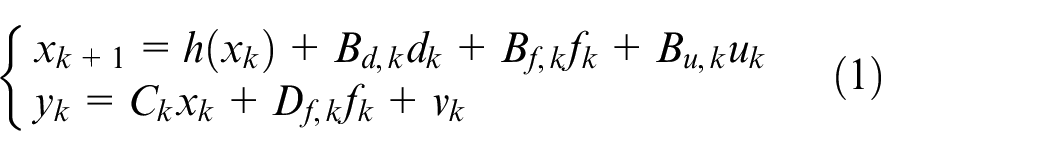
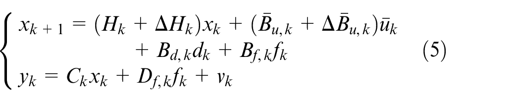
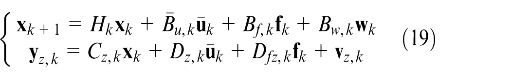
Consider the following time-variant nonlinear systems

{\begin{matrix} x_{k + 1} = h (x_{k}) + B_{d, k} d_{k} + B_{f, k} f_{k} + B_{u, k} u_{k} \\ y_{k} = C_{k} x_{k} + D_{f, k} f_{k} + v_{k} \end{matrix}

(1)

where $x_{k} \in R^{n_{x}}$ , $y_{k} \in R^{n_{y}}$ , $u_{k} \in R^{n_{u}}$ , $d_{k} \in R^{n_{d}}$ , $v_{k} \in R^{n_{v}}$ , and $f_{k} \in R^{n_{f}}$ denote the state, measurement, controlled input, process disturbance, measurement noise, and the fault signal to be reconstructed, respectively. Here, the signals $f_{k}$ , $d_{k}$ , and $v_{k}$ are assumed to be with bounded $l_{2}$ norms. $B_{d, k}$ , $B_{f, k}$ , $B_{u, k}$ , $C_{k}$ , and $D_{f, k}$ are known time-varying matrices with appropriate dimensions. The initial state is assumed to be $x_{0}$ . The nonlinear function $h (x_{k})$ is assumed to be continuously differentiable (with standard regularity).^25,26

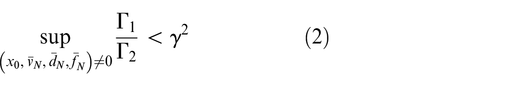
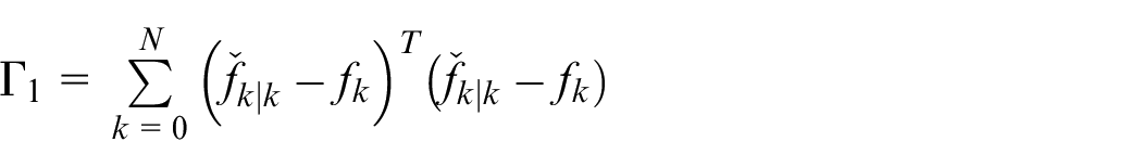
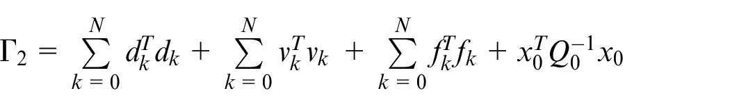
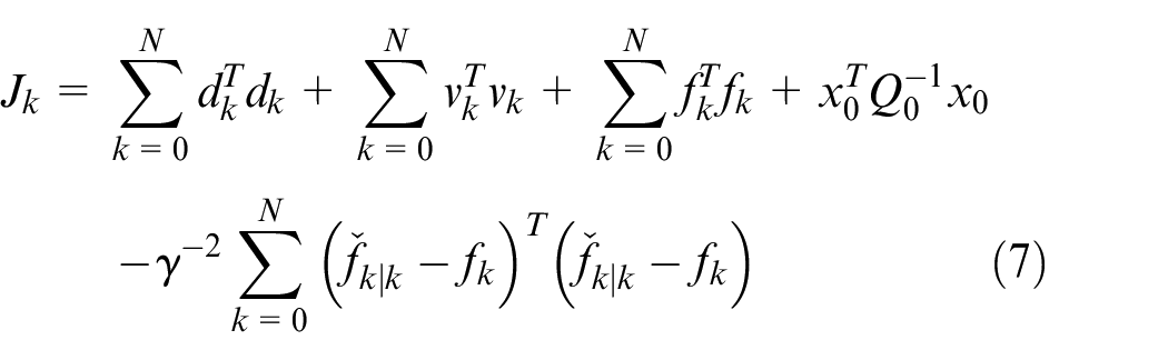
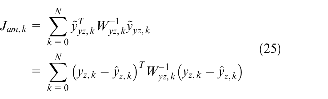
For system (1), our main objective of this study is to find ${\overset{\lor}{f}}_{k | k}$ serving as an estimation of the fault $f_{k}$ using the measurement set ${y_{0}, \dots, y_{k}}$ so as to fulfill the following $H_{\infty}$ index

sup_{(x_{0}, {\bar{v}}_{N}, {\bar{d}}_{N}, {\bar{f}}_{N}) \neq 0} \frac{Γ_{1}}{Γ_{2}} < γ^{2}

(2)

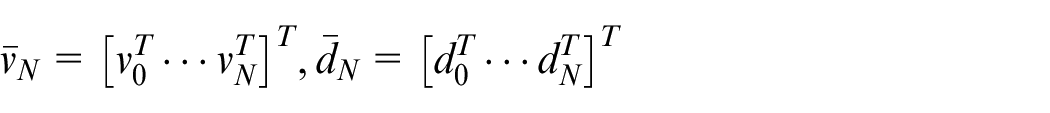
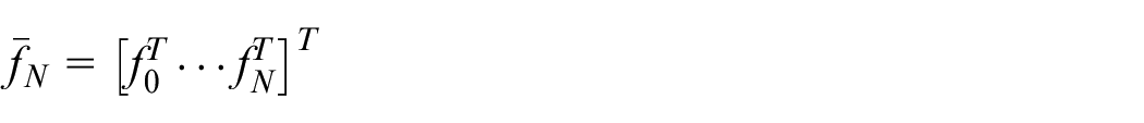
where

{\bar{v}}_{N} = {[v_{0}^{T} \dots v_{N}^{T}]}^{T}, {\bar{d}}_{N} = {[d_{0}^{T} \dots d_{N}^{T}]}^{T}

{\bar{f}}_{N} = {[f_{0}^{T} \dots f_{N}^{T}]}^{T}

Γ_{1} = \sum_{k = 0}^{N} {({\overset{ˇ}{f}}_{k | k} - f_{k})}^{T} ({\overset{ˇ}{f}}_{k | k} - f_{k})

Γ_{2} = \sum_{k = 0}^{N} d_{k}^{T} d_{k} + \sum_{k = 0}^{N} v_{k}^{T} v_{k} + \sum_{k = 0}^{N} f_{k}^{T} f_{k} + x_{0}^{T} Q_{0}^{- 1} x_{0}

here, $γ$ represents a given disturbance attenuation ratio and $Q_{0}$ a weighting positive matrix.

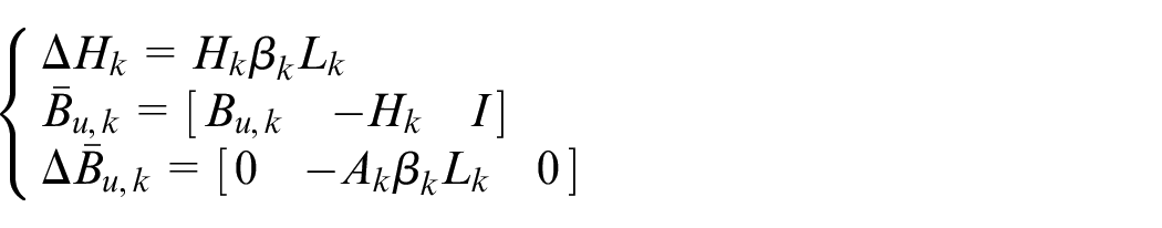
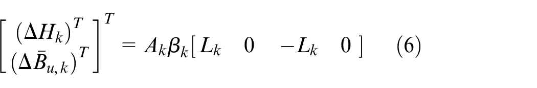
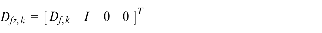
To achieve our goal, a dynamic filter which plays the role of the estimator is needed. To proceed, we first expand $h (x_{k})$ in Taylor series about ${\hat{x}}_{k}$ in the following way

{\begin{matrix} x_{k + 1} = H_{k} (x_{k} - {\hat{x}}_{k}) + f ({\hat{x}}_{k}) + B_{d, k} d_{k} + B_{f, k} f_{k} \\ + B_{u, k} u_{k} + A_{k} β_{k} L_{k} (x_{k} - {\hat{x}}_{k}) \\ y_{k} = C_{k} x_{k} + D_{f, k} f_{k} + v_{k} \end{matrix}

(3)

where ${H_{k} = \frac{\partial h (x)}{\partial x} |}_{x = {\hat{x}}_{k}}$ and ${\hat{x}}_{k}$ is the state variable of the filter (estimator). $A_{k} \in R^{n_{x} \times n_{x}}$ is a problem-dependent scaling matrix and $β_{k} \in R^{n_{x} \times n_{x}}$ is an unknown time-varying parameter matrix used to consider the linearization errors of the dynamic model. $β_{k}$ is assumed to be bounded as follows

β_{k}^{T} β_{k} \leq I

(4)

The matrix $L_{k} \in R^{n_{x} \times n_{x}}$ is given to provide an extra degree of freedom in purpose of tuning the estimator.²⁶

Define

{\bar{u}}_{k} = [\begin{matrix} u_{k} \\ {\hat{x}}_{k} \\ f ({\hat{x}}_{k}) \end{matrix}]

and

{\begin{matrix} Δ H_{k} = H_{k} β_{k} L_{k} \\ {\bar{B}}_{u, k} = [\begin{matrix} B_{u, k} & - H_{k} & I \end{matrix}] \\ Δ {\bar{B}}_{u, k} = [\begin{matrix} 0 & - A_{k} β_{k} L_{k} & 0 \end{matrix}] \end{matrix}

Equation (3) can be rewritten as

{\begin{matrix} x_{k + 1} = (H_{k} + Δ H_{k}) x_{k} + ({\bar{B}}_{u, k} + Δ {\bar{B}}_{u, k}) {\bar{u}}_{k} \\ + B_{d, k} d_{k} + B_{f, k} f_{k} \\ y_{k} = C_{k} x_{k} + D_{f, k} f_{k} + v_{k} \end{matrix}

(5)

with

{[\begin{matrix} {(Δ H_{k})}^{T} \\ {(Δ {\bar{B}}_{u, k})}^{T} \end{matrix}]}^{T} = A_{k} β_{k} [\begin{matrix} L_{k} & 0 & \begin{matrix} - L_{k} & 0 \end{matrix} \end{matrix}]

(6)

Thus, the original time-variant nonlinear system (1) is transformed into a linear form by taking the linearization error into account, where this error refers to the high-order terms of the Taylor series expansion and is modeled by norm-bounded uncertain matrix.

Traditionally speaking, for the purpose of designing an appropriate ${\overset{\lor}{f}}_{k | k}$ to satisfy the index (2), a direct way is to solve a quadratic optimization problem in the following two steps:^27–29

Step 1: To guarantee the following transferred performance index $J_{k}$ that corresponds to index (2) has a minimum over $(x_{0}, {\bar{v}}_{N}, {\bar{d}}_{N}, {\bar{f}}_{N})$

\begin{matrix} J_{k} = \sum_{k = 0}^{N} d_{k}^{T} d_{k} + \sum_{k = 0}^{N} v_{k}^{T} v_{k} + \sum_{k = 0}^{N} f_{k}^{T} f_{k} + x_{0}^{T} Q_{0}^{- 1} x_{0} - γ^{- 2} \sum_{k = 0}^{N} {({\overset{\lor}{f}}_{k | k} - f_{k})}^{T} ({\overset{\lor}{f}}_{k | k} - f_{k}) \end{matrix}

(7)

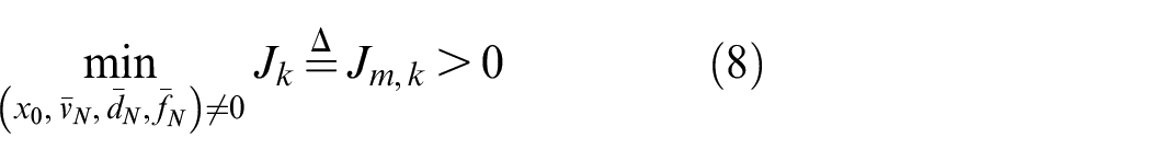
Step 2: Choose ${\overset{\lor}{f}}_{k | k}$ such that the value of $J_{k}$ in system (7) at its minimum is positive, that is

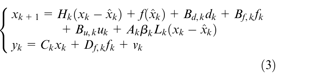
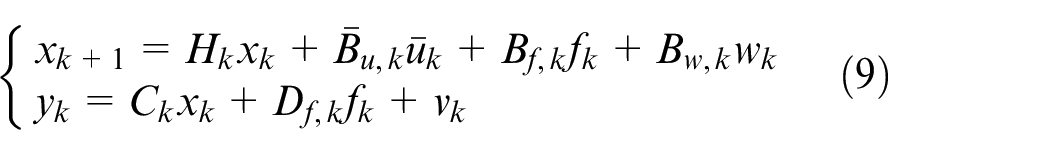
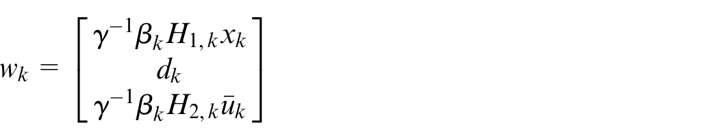
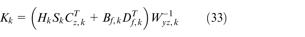
min_{(x_{0}, {\bar{v}}_{N}, {\bar{d}}_{N}, {\bar{f}}_{N}) \neq 0} J_{k} =^{Δ} J_{m, k} > 0

(8)

Observing the fact that the converted system includes uncertain matrices $Δ H_{k}$ and $Δ {\bar{B}}_{u, k}$ in equation (6), to find a suitable ${\overset{\lor}{f}}_{k | k}$ that satisfies equation (8) or the original performance index (2), we construct an equivalent form of equation (5) as follows

{\begin{matrix} x_{k + 1} = H_{k} x_{k} + {\bar{B}}_{u, k} {\bar{u}}_{k} + B_{f, k} f_{k} + B_{w, k} w_{k} \\ y_{k} = C_{k} x_{k} + D_{f, k} f_{k} + v_{k} \end{matrix}

(9)

with

B_{w, k} = [\begin{matrix} γ E_{1, k} & B_{d, k} & γ E_{2, k} \end{matrix}]

H_{1, k} = L_{k}

H_{2, k} = [\begin{matrix} 0 & - L_{k} & 0 \end{matrix}]

w_{k} = [\begin{matrix} γ^{- 1} β_{k} H_{1, k} x_{k} \\ d_{k} \\ γ^{- 1} β_{k} H_{2, k} {\bar{u}}_{k} \end{matrix}]

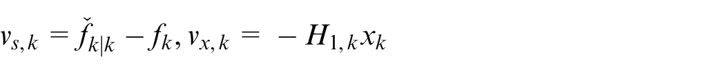
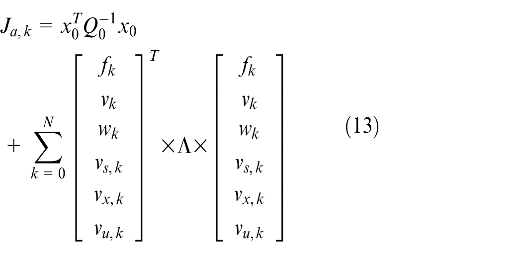
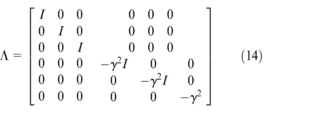
For system (9), let

v_{s, k} = {\overset{\lor}{f}}_{k | k} - f_{k}, v_{x, k} = - H_{1, k} x_{k}

v_{u, k} = - H_{2, k} {\bar{u}}_{k}

r_{a, k} = {[\begin{matrix} v_{s, k}^{T} & v_{u, k}^{T} & v_{x, k}^{T} \end{matrix}]}^{T}

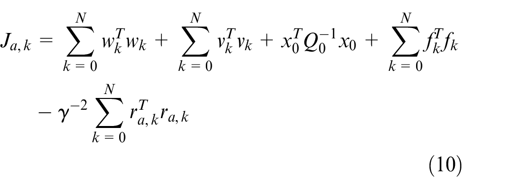
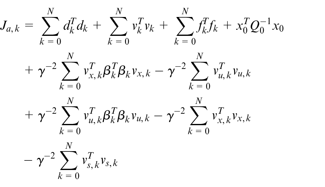
and define the following alternative performance function $J_{a, k}$

\begin{matrix} J_{a, k} = \sum_{k = 0}^{N} w_{k}^{T} w_{k} + \sum_{k = 0}^{N} v_{k}^{T} v_{k} + x_{0}^{T} Q_{0}^{- 1} x_{0} + \sum_{k = 0}^{N} f_{k}^{T} f_{k} \\ - γ^{- 2} \sum_{k = 0}^{N} r_{a, k}^{T} r_{a, k} \end{matrix}

(10)

Then, we get the following lemma.

Lemma 1

Given any $γ > 0$ , for systems (5) and (9), we have

J_{a, k} \leq J_{k}

(11)

Proof

From system (10), we can get

\begin{matrix} J_{a, k} = \sum_{k = 0}^{N} d_{k}^{T} d_{k} + \sum_{k = 0}^{N} v_{k}^{T} v_{k} + \sum_{k = 0}^{N} f_{k}^{T} f_{k} + x_{0}^{T} Q_{0}^{- 1} x_{0} \\ + γ^{- 2} \sum_{k = 0}^{N} v_{x, k}^{T} β_{k}^{T} β_{k} v_{x, k} - γ^{- 2} \sum_{k = 0}^{N} v_{u, k}^{T} v_{u, k} \\ + γ^{- 2} \sum_{k = 0}^{N} v_{u, k}^{T} β_{k}^{T} β_{k} v_{u, k} - γ^{- 2} \sum_{k = 0}^{N} v_{x, k}^{T} v_{x, k} \\ - γ^{- 2} \sum_{k = 0}^{N} v_{s, k}^{T} v_{s, k} \end{matrix}

Thus, through equation (4), we can deduce equation (11) holds. □

Denote $J_{am, k}$ as the minimum of $J_{a, k}$ . Based on Lemma 1, a corollary can be addressed as follows.

Corollary 1

Given any $γ > 0$ , for systems (5) and (9), we get

J_{am, k} |_{L_{k} = 0} = J_{m, k}

From Lemma 1 and Corollary 1, we know that $J_{a, k}$ is a lower bound of $J_{k}$ , and $J_{a, k}$ has the same minimum with $J_{k}$ when $L_{k} = 0$ (only for $J_{a, k}$ ). Note that the uncertainty in system (5) is rearranged with respect to the alternative system (9) with $J_{a, k}$ . Therefore, due to Lemma 1 and Corollary 1, the key to construct ${\overset{\lor}{f}}_{k | k}$ is to search $J_{am, k}$ in order that $J_{am, k} |_{L_{k} = 0} = J_{m, k} > 0$ . As a result, the $H_{\infty}$ fault estimation issue is formulated as Problem 1 in two stages.

Problem 1

To ensure $J_{a, k}$ has a minimum over $(x_{0}, {\bar{v}}_{N}, {\bar{d}}_{N}, {\bar{f}}_{N})$ with $w_{N} = [\begin{matrix} w_{0}^{T} & \dots & w_{N}^{T} \end{matrix}]^{T}$ ;

To choose a suitable ${\overset{\lor}{f}}_{k | k}$ such that $J_{am, k} |_{L_{k} = 0} = J_{m, k} > 0$ .

In virtue of Hassibi et al.²⁷ and Zhao et al.,²⁹ Problem 1 can be transformed into a linear estimation problem in indefinite inner product space, namely, Krein space. In other words, we need to build a model in this space with regard to system (9); find the minimum of $J_{a, k}$ through linear estimation technique; and then select a suitable ${\overset{\lor}{f}}_{k | k}$ such that $J_{am, k} |_{L_{k} = 0} = J_{m, k} > 0$ .

Main results

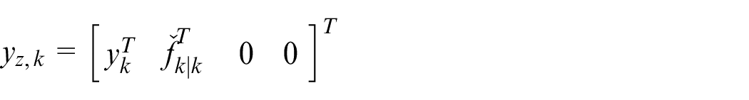
To continue, we preliminarily introduce the following model through defining a fictitious output

\begin{matrix} x_{k + 1} = H_{k} x_{k} + {\bar{B}}_{u, k} {\bar{u}}_{k} + B_{f, k} f_{k} + B_{w, k} w_{k} \\ y_{z, k} = C_{z, k} x_{k} + D_{z, k} {\bar{u}}_{k} + D_{fz, k} f_{k} + v_{z, k} \end{matrix}

(12)

where

y_{z, k} = {[\begin{matrix} y_{k}^{T} & {\overset{\lor}{f}}_{k | k}^{T} & \begin{matrix} 0 & 0 \end{matrix} \end{matrix}]}^{T}

v_{z, k} = {[\begin{matrix} v_{k}^{T} & v_{s, k}^{T} & \begin{matrix} v_{x, k}^{T} & v_{u, k}^{T} \end{matrix} \end{matrix}]}^{T}

C_{z, k} = {[\begin{matrix} C_{k}^{T} & 0 & \begin{matrix} H_{1, k}^{T} & 0 \end{matrix} \end{matrix}]}^{T}

D_{z, k} = {[\begin{matrix} 0 & 0 & \begin{matrix} 0 & H_{2, k} \end{matrix} \end{matrix}]}^{T}

D_{fz, k} = {[\begin{matrix} D_{f, k} & I & \begin{matrix} 0 & 0 \end{matrix} \end{matrix}]}^{T}

Remember that

\begin{matrix} J_{a, k} = x_{0}^{T} Q_{0}^{- 1} x_{0} \\ + \sum_{k = 0}^{N} {[\begin{matrix} f_{k} \\ v_{k} \\ \begin{matrix} w_{k} \\ v_{s, k} \\ \begin{matrix} v_{x, k} \\ v_{u, k} \end{matrix} \end{matrix} \end{matrix}]}^{T} \times Λ \times [\begin{matrix} f_{k} \\ v_{k} \\ \begin{matrix} w_{k} \\ v_{s, k} \\ \begin{matrix} v_{x, k} \\ v_{u, k} \end{matrix} \end{matrix} \end{matrix}] \end{matrix}

(13)

where

Λ = [\begin{matrix} \begin{matrix} I & 0 & 0 \\ 0 & I & 0 \\ 0 & 0 & I \end{matrix} & \begin{matrix} 0 & 0 & 0 \\ 0 & 0 & 0 \\ 0 & 0 & 0 \end{matrix} \\ \begin{matrix} 0 & 0 & 0 \\ 0 & 0 & 0 \\ 0 & 0 & 0 \end{matrix} & \begin{matrix} - γ^{2} I & 0 & 0 \\ 0 & - γ^{2} I & 0 \\ 0 & 0 & - γ^{2} \end{matrix} \end{matrix}]

(14)

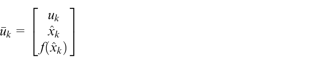
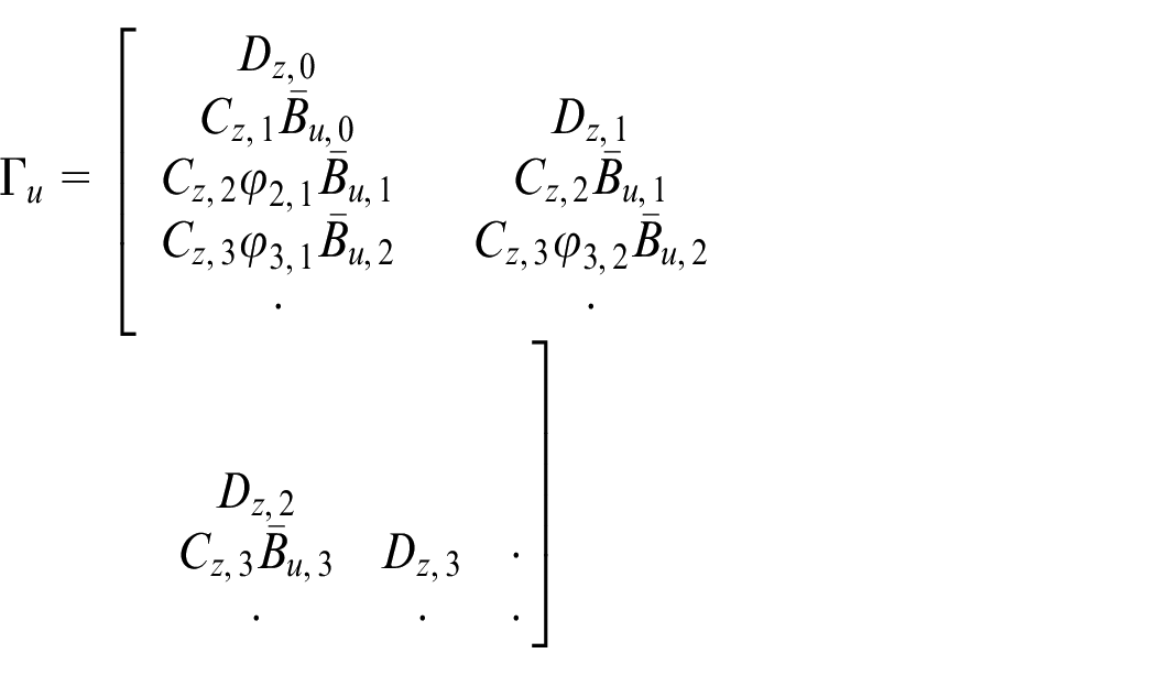
Thus, by using the following notations

\begin{matrix} {\bar{f}}_{N} = {[\begin{matrix} f_{0}^{T} & \dots & f_{N}^{T} \end{matrix}]}^{T} \\ {\bar{w}}_{N} = {[\begin{matrix} w_{0}^{T} & \dots & w_{N}^{T} \end{matrix}]}^{T} \\ {\bar{v}}_{z, N} = {[\begin{matrix} v_{z, 0}^{T} & \dots & v_{z, N}^{T} \end{matrix}]}^{T} \end{matrix}

$J_{a, k}$ can be re-expressed as

J_{a, k} = {[\begin{matrix} x_{0} \\ {\bar{f}}_{N} \\ \begin{matrix} {\bar{w}}_{N} \\ {\bar{v}}_{z, N} \end{matrix} \end{matrix}]}^{T} {[\begin{matrix} \begin{matrix} Q_{0} & 0 \\ 0 & I \end{matrix} & \begin{matrix} 0 & 0 \\ 0 & 0 \end{matrix} \\ \begin{matrix} 0 & 0 \\ 0 & 0 \end{matrix} & \begin{matrix} I & 0 \\ 0 & \bar{Π} \end{matrix} \end{matrix}]}^{- 1} [\begin{matrix} x_{0} \\ {\bar{f}}_{N} \\ \begin{matrix} {\bar{w}}_{N} \\ {\bar{v}}_{z, N} \end{matrix} \end{matrix}]

(15)

where $\bar{Π} = Π_{0} \oplus \dots \oplus Π_{N}$ , with $Π_{k} = diag {I, - γ^{2} I, - γ^{2} I, - γ^{2} I}$ .

Let

{\bar{y}}_{z, N} = {[\begin{matrix} y_{z, 0}^{T} & \dots & y_{z, N}^{T} \end{matrix}]}^{T}, {\tilde{u}}_{N} = {[\begin{matrix} {\bar{u}}_{0}^{T} & \dots & {\bar{u}}_{N}^{T} \end{matrix}]}^{T}

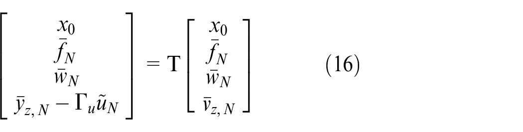
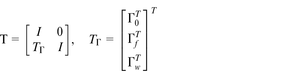
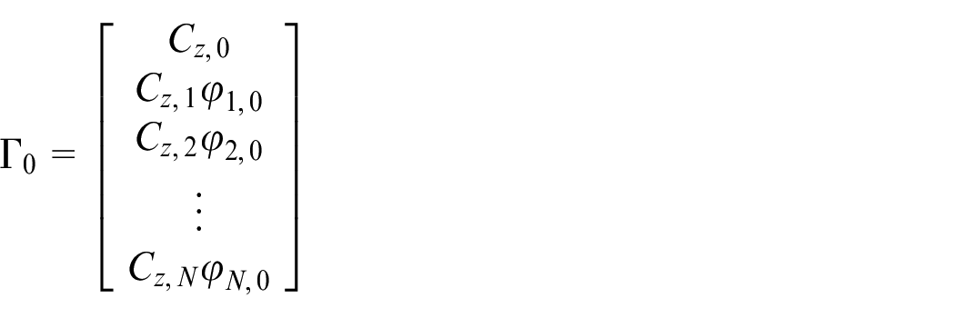
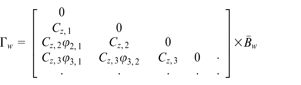
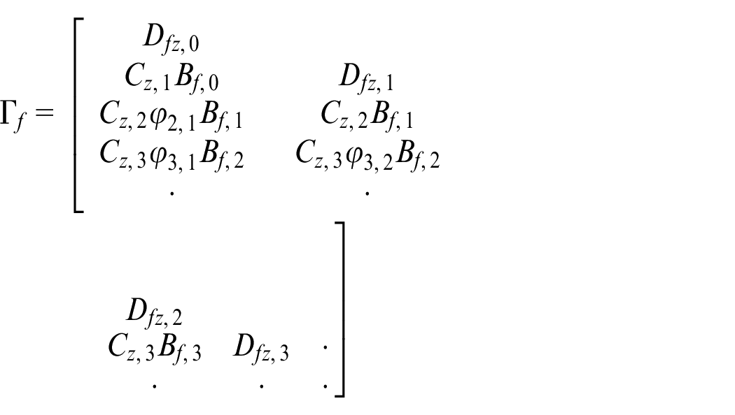
and denote $φ_{i, j}$ as the transition matrix of system (12) from time instant $j$ to $i$ ; then, we have

[\begin{matrix} x_{0} \\ {\bar{f}}_{N} \\ \begin{matrix} {\bar{w}}_{N} \\ {\bar{y}}_{z, N} - Γ_{u} {\tilde{u}}_{N} \end{matrix} \end{matrix}] = T [\begin{matrix} x_{0} \\ {\bar{f}}_{N} \\ \begin{matrix} {\bar{w}}_{N} \\ {\bar{v}}_{z, N} \end{matrix} \end{matrix}]

(16)

here, $T$ is the operator mapping $[\begin{matrix} x_{0}^{T} & {\bar{f}}_{N}^{T} & \begin{matrix} {\bar{w}}_{N}^{T} & {\bar{v}}_{z, N}^{T} \end{matrix} \end{matrix}]^{T}$ to $[\begin{matrix} x_{0}^{T} & {\bar{f}}_{N}^{T} & \begin{matrix} {\bar{w}}_{N}^{T} & {({\bar{y}}_{z, N} - Γ_{u} {\tilde{u}}_{N})}^{T} \end{matrix} \end{matrix}]^{T}$ with

T = [\begin{matrix} I & 0 \\ T_{Γ} & I \end{matrix}], T_{Γ} = {[\begin{matrix} Γ_{0}^{T} \\ Γ_{f}^{T} \\ Γ_{w}^{T} \end{matrix}]}^{T}

Γ_{0} = [\begin{matrix} C_{z, 0} \\ C_{z, 1} φ_{1, 0} \\ \begin{matrix} C_{z, 2} φ_{2, 0} \\ ⋮ \\ C_{z, N} φ_{N, 0} \end{matrix} \end{matrix}]

Γ_{w} = [\begin{matrix} 0 & \begin{matrix}  \end{matrix} \\ C_{z, 1} & 0 & \begin{matrix}  \end{matrix} \\ \begin{matrix} C_{z, 2} φ_{2, 1} \\ C_{z, 3} φ_{3, 1} \\ \cdot \end{matrix} & \begin{matrix} C_{z, 2} \\ C_{z, 3} φ_{3, 2} \\ \cdot \end{matrix} & \begin{matrix} \begin{matrix} 0 \\ C_{z, 3} \\ \cdot \end{matrix} & \begin{matrix} 0 \\ \cdot \end{matrix} & \begin{matrix} \cdot \\ \cdot \end{matrix} \end{matrix} \end{matrix}] \times {\bar{B}}_{w}

{\bar{B}}_{w} = diag {B_{w, 0}, B_{w, 1}, \dots, B_{w, N}}

\begin{matrix} Γ_{f} = [\begin{matrix} \begin{matrix} D_{fz, 0} \\ C_{z, 1} B_{f, 0} \\ \begin{matrix} C_{z, 2} φ_{2, 1} B_{f, 1} \\ C_{z, 3} φ_{3, 1} B_{f, 2} \\ \cdot \end{matrix} \end{matrix} & \begin{matrix} D_{fz, 1} \\ \begin{matrix} C_{z, 2} B_{f, 1} \\ C_{z, 3} φ_{3, 2} B_{f, 2} \\ \cdot \end{matrix} \end{matrix} \end{matrix} \\ \begin{matrix} \begin{matrix} D_{fz, 2} \end{matrix} & \begin{matrix}  \end{matrix} & \begin{matrix}  \end{matrix} \\ C_{z, 3} B_{f, 3} & D_{fz, 3} & \cdot \\ \cdot & \cdot & \cdot \end{matrix}] \end{matrix}

\begin{matrix} Γ_{u} = [\begin{matrix} \begin{matrix} D_{z, 0} \\ C_{z, 1} {\bar{B}}_{u, 0} \\ \begin{matrix} C_{z, 2} φ_{2, 1} {\bar{B}}_{u, 1} \\ C_{z, 3} φ_{3, 1} {\bar{B}}_{u, 2} \\ \cdot \end{matrix} \end{matrix} & \begin{matrix} D_{z, 1} \\ \begin{matrix} C_{z, 2} {\bar{B}}_{u, 1} \\ C_{z, 3} φ_{3, 2} {\bar{B}}_{u, 2} \\ \cdot \end{matrix} \end{matrix} \end{matrix} \\ \begin{matrix} \begin{matrix} D_{z, 2} \end{matrix} & \begin{matrix}  \end{matrix} & \begin{matrix}  \end{matrix} \\ C_{z, 3} {\bar{B}}_{u, 3} & D_{z, 3} & \cdot \\ \cdot & \cdot & \cdot \end{matrix}] \end{matrix}

Let

Ω = [\begin{matrix} Q_{0} & 0 & \begin{matrix} 0 & 0 \end{matrix} \\ 0 & I & \begin{matrix} 0 & 0 \end{matrix} \\ \begin{matrix} 0 \\ 0 \end{matrix} & \begin{matrix} 0 \\ 0 \end{matrix} & \begin{matrix} \begin{matrix} I & 0 \end{matrix} \\ \begin{matrix} 0 & \bar{Π} \end{matrix} \end{matrix} \end{matrix}]

(17)

Since $T$ is invertible, we know that

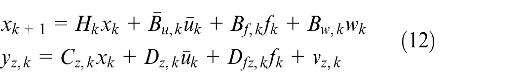
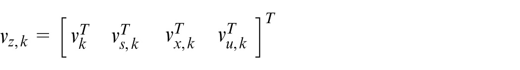
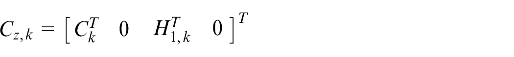
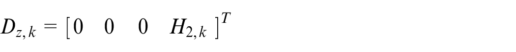
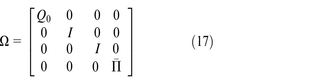
\begin{matrix} J_{a, k} = {[\begin{matrix} x_{0} \\ {\bar{f}}_{N} \\ \begin{matrix} {\bar{w}}_{N} \\ {\bar{v}}_{z, N} \end{matrix} \end{matrix}]}^{T} Ω^{- 1} [\begin{matrix} x_{0} \\ {\bar{f}}_{N} \\ \begin{matrix} {\bar{w}}_{N} \\ {\bar{v}}_{z, N} \end{matrix} \end{matrix}] \\ = {[\begin{matrix} x_{0} \\ {\bar{f}}_{N} \\ \begin{matrix} {\bar{w}}_{N} \\ {\bar{y}}_{z, N} - Γ_{u} {\tilde{u}}_{N} \end{matrix} \end{matrix}]}^{T} T^{- T} Ω^{- 1} T^{- 1} \times [\begin{matrix} x_{0} \\ {\bar{f}}_{N} \\ \begin{matrix} {\bar{w}}_{N} \\ {\bar{y}}_{z, N} - Γ_{u} {\tilde{u}}_{N} \end{matrix} \end{matrix}] \\ = {[\begin{matrix} x_{0} \\ {\bar{f}}_{N} \\ \begin{matrix} {\bar{w}}_{N} \\ {\bar{y}}_{z, N} - Γ_{u} {\tilde{u}}_{N} \end{matrix} \end{matrix}]}^{T} {(T Ω T^{T})}^{- 1} \times [\begin{matrix} x_{0} \\ {\bar{f}}_{N} \\ \begin{matrix} {\bar{w}}_{N} \\ {\bar{y}}_{z, N} - Γ_{u} {\tilde{u}}_{N} \end{matrix} \end{matrix}] \end{matrix}

(18)

In terms of systems (12)–(18) and according to Hassibi et al.²⁷ and Zhao et al.,²⁹ we can introduce the following Krein space stochastic system to settle Problem 1

{\begin{matrix} x_{k + 1} = H_{k} x_{k} + {\bar{B}}_{u, k} {\bar{u}}_{k} + B_{f, k} f_{k} + B_{w, k} w_{k} \\ y_{z, k} = C_{z, k} x_{k} + D_{z, k} {\bar{u}}_{k} + D_{fz, k} f_{k} + v_{z, k} \end{matrix}

(19)

where

y_{z, k} = [\begin{matrix} C_{k} \\ 0 \\ \begin{matrix} H_{1, k} \\ 0 \end{matrix} \end{matrix}] x_{k} + [\begin{matrix} 0 \\ 0 \\ \begin{matrix} 0 \\ H_{2, k} \end{matrix} \end{matrix}] {\bar{u}}_{k} + [\begin{matrix} D_{f, k} \\ I \\ \begin{matrix} 0 \\ 0 \end{matrix} \end{matrix}] f_{k} + [\begin{matrix} v_{k} \\ v_{s, k} \\ \begin{matrix} v_{x, k} \\ v_{u, k} \end{matrix} \end{matrix}]

(20)

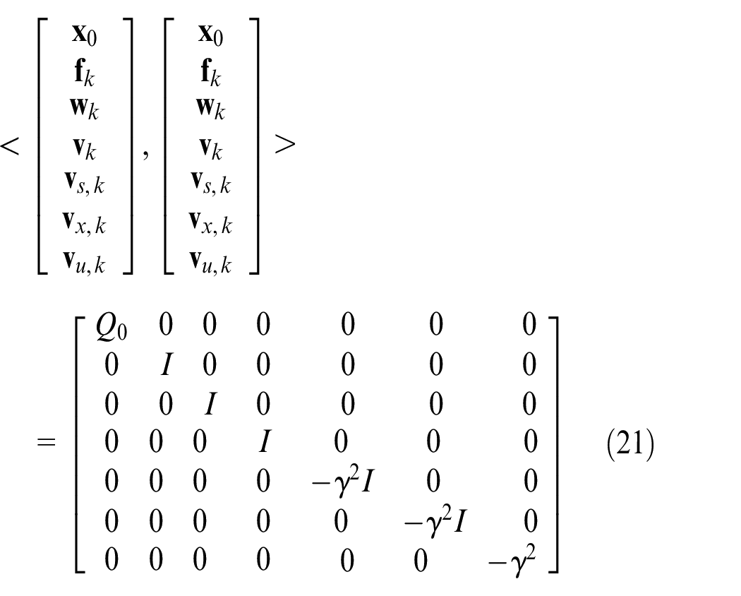
with $C_{z, k} = [\begin{matrix} C_{k}^{T} & 0 & \begin{matrix} H_{1, k}^{T} & 0 \end{matrix} \end{matrix}]^{T}$ , $D_{z, k} = [\begin{matrix} 0 & 0 & \begin{matrix} 0 & H_{2, k}^{T} \end{matrix} \end{matrix}]^{T}$ , and $D_{fz, k} = [\begin{matrix} D_{f, k}^{T} & I & \begin{matrix} 0 & 0 \end{matrix} \end{matrix}]^{T}$ , which are identical to the related matrix quantities given in system (12). Here, $f_{k}, w_{k}, v_{z, k} = [\begin{matrix} v_{k}^{T} & v_{s, k}^{T} & \begin{matrix} v_{x, k}^{T} & v_{u, k}^{T} \end{matrix} \end{matrix}]^{T}$ as well as the initial state $x_{0}$ are all random variables with zero means, and their covariances are shown below

< [\begin{matrix} x_{0} \\ f_{k} \\ \begin{matrix} w_{k} \\ v_{k} \\ \begin{matrix} v_{s, k} \\ v_{x, k} \\ v_{u, k} \end{matrix} \end{matrix} \end{matrix}], [\begin{matrix} x_{0} \\ f_{k} \\ \begin{matrix} w_{k} \\ v_{k} \\ \begin{matrix} v_{s, k} \\ v_{x, k} \\ v_{u, k} \end{matrix} \end{matrix} \end{matrix}] > = [\begin{matrix} \begin{matrix} Q_{0} & 0 & 0 \\ 0 & I & 0 \\ 0 & 0 & I \end{matrix} & \begin{matrix} 0 \\ 0 \\ 0 \end{matrix} & \begin{matrix} 0 & 0 & 0 \\ 0 & 0 & 0 \\ 0 & 0 & 0 \end{matrix} \\ \begin{matrix} 0 & 0 & 0 \\ 0 & 0 & 0 \\ 0 & 0 & 0 \end{matrix} & \begin{matrix} I \\ 0 \\ 0 \end{matrix} & \begin{matrix} 0 & 0 & 0 \\ - γ^{2} I & 0 & 0 \\ 0 & - γ^{2} I & 0 \end{matrix} \\ \begin{matrix} 0 & 0 & 0 \end{matrix} & 0 & \begin{matrix} 0 & 0 & - γ^{2} \end{matrix} \end{matrix}]

(21)

Based on systems (19) and (20), we can define some related variables below

e_{k} = x_{k} - {\hat{x}}_{k}, S_{k} = e_{k}, e_{k}

with

{\tilde{y}}_{z, k} = y_{z, k} - {\hat{y}}_{z, k}

(22)

and

{\hat{y}}_{z, k} = C_{z, k} {\hat{x}}_{k} + D_{z, k} u_{k}

where ${\hat{x}}_{k}$ denotes the projection of $x_{k}$ onto $L {{y_{z, j}}_{j = 0}^{k - 1}}$ .

Let

Q_{vz, k} = [\begin{matrix} I & 0 & \begin{matrix} 0 & 0 \end{matrix} \\ 0 & - γ^{2} I & \begin{matrix} 0 & 0 \end{matrix} \\ \begin{matrix} 0 \\ 0 \end{matrix} & \begin{matrix} 0 \\ 0 \end{matrix} & \begin{matrix} \begin{matrix} - γ^{2} I \\ 0 \end{matrix} & \begin{matrix} 0 \\ - γ^{2} I \end{matrix} \end{matrix} \end{matrix}]

(23)

and define $W_{yz, k} = 〈 {\tilde{y}}_{z, k}, {\tilde{y}}_{z, k} 〉$ . In terms of systems (19)–(22), we have

\begin{matrix} W_{yz, k} = C_{z, k} S_{k} C_{z, k}^{T} + D_{zf, k} D_{zf, k}^{T} + Q_{vz, k} \\ = [\begin{matrix} C_{k} \\ 0 \\ \begin{matrix} L_{k} \\ 0 \end{matrix} \end{matrix}] S_{k} [\begin{matrix} C_{k}^{T} & 0 & \begin{matrix} L_{k}^{T} & 0 \end{matrix} \end{matrix}] \\ + [\begin{matrix} D_{f, k} D_{f, k}^{T} & D_{f, k} & \begin{matrix} 0 & 0 \end{matrix} \\ D_{f, k}^{T} & I & \begin{matrix} 0 & 0 \end{matrix} \\ \begin{matrix} 0 \\ 0 \end{matrix} & \begin{matrix} 0 \\ 0 \end{matrix} & \begin{matrix} \begin{matrix} 0 & 0 \end{matrix} \\ \begin{matrix} 0 & 0 \end{matrix} \end{matrix} \end{matrix}] \\ + [\begin{matrix} I & 0 & \begin{matrix} 0 & 0 \end{matrix} \\ 0 & - γ^{2} I & \begin{matrix} 0 & 0 \end{matrix} \\ \begin{matrix} 0 \\ 0 \end{matrix} & \begin{matrix} 0 \\ 0 \end{matrix} & \begin{matrix} \begin{matrix} - γ^{2} I \\ 0 \end{matrix} & \begin{matrix} 0 \\ - γ^{2} I \end{matrix} \end{matrix} \end{matrix}] \end{matrix}

(24)

\begin{matrix} = \begin{matrix} [\begin{matrix} C_{k} S_{k} C_{k}^{T} + D_{f, k} D_{f, k}^{T} + I \\ D_{f, k}^{T} \\ \begin{matrix} L_{k} C_{k}^{T} \\ 0 \end{matrix} \end{matrix} \\ \begin{matrix} D_{f, k} & C_{k} L_{k}^{T} & 0 \\ I - γ^{2} I & 0 & 0 \\ \begin{matrix} 0 \\ 0 \end{matrix} & \begin{matrix} L_{k} L_{k}^{T} - γ^{2} I \\ 0 \end{matrix} & \begin{matrix} 0 \\ - γ^{2} I \end{matrix} \end{matrix}] \end{matrix} \end{matrix}

From the analysis above and according to Hassibi et al.,²⁷ we can draw the following result, which is summarized as Corollary 2.

Corollary 2

For system (9) and a given perturbation attenuation ratio $γ > 0$ , $J_{a, k}$ has the minimum over the set $(x_{0}, {\bar{v}}_{N}, {\bar{w}}_{N}, {\bar{f}}_{N})$ , if and only if (iff) $Q_{vz, k}$ and $W_{yz, k}$ have the same inertia. In such a case, the minimum of $J_{a, k}$ , namely $J_{am, k}$ , is calculated by

\begin{matrix} J_{am, k} = \sum_{k = 0}^{N} {\tilde{y}}_{yz, k}^{T} W_{yz, k}^{- 1} {\tilde{y}}_{yz, k} \\ = \sum_{k = 0}^{N} {(y_{z, k} - {\hat{y}}_{z, k})}^{T} W_{yz, k}^{- 1} (y_{z, k} - {\hat{y}}_{z, k}) \end{matrix}

(25)

where

{\hat{y}}_{z, k} = C_{z, k} {\hat{x}}_{k} + D_{z, k} {\bar{u}}_{k}

here, ${\hat{x}}_{k}$ is computed by the projections of $x_{k}$ on $L {{y_{z, j}}_{j = 0}^{k - 1}}$ in Krein space.

Based on Corollary 2, we are ready to choose an appropriate function of the measurement set ${y_{0}, \dots, y_{k}}$ as ${\overset{\lor}{f}}_{k | k}$ to guarantee $J_{am, k} |_{L_{k} = 0} = J_{m, k} > 0$ . Theorem 1 provides one choice of ${\overset{\lor}{f}}_{k | k}$ to achieve our goal.

Theorem 1

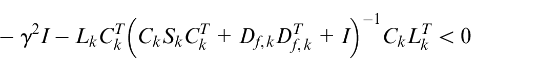
For system (9) and a given perturbation attenuation ratio $γ > 0$ , the fault estimator that fulfills the performance index (2) exists, iff

C_{k} S_{k} C_{k}^{T} + D_{f, k} D_{f, k}^{T} + I > 0

- γ^{2} I - L_{k} C_{k}^{T} {(C_{k} S_{k} C_{k}^{T} + D_{f, k} D_{f, k}^{T} + I)}^{- 1} C_{k} L_{k}^{T} < 0

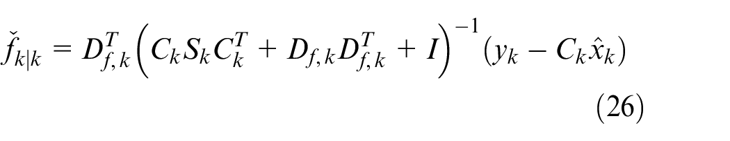
In such a case, one choice of ${\overset{\lor}{f}}_{k | k}$ is given as

{\overset{\lor}{f}}_{k | k} = D_{f, k}^{T} {(C_{k} S_{k} C_{k}^{T} + D_{f, k} D_{f, k}^{T} + I)}^{- 1} (y_{k} - C_{k} {\hat{x}}_{k})

(26)

where ${\hat{x}}_{k}$ is computed by the projections of $x_{k}$ on $L {{y_{z, j}}_{j = 0}^{k - 1}}$ in Krein space.

Proof

Let

\tilde{A} = C_{k} S_{k} C_{k}^{T} + D_{f, k} D_{f, k}^{T} + I

\tilde{B} = C_{k} L_{k}^{T}

\tilde{D} = - γ^{2} I

Thus, $W_{yz, k}$ in system (24) can be rewritten as

W_{yz, k} = [\begin{matrix} I & 0 \\ {\tilde{B}}^{T} {\tilde{A}}^{- 1} & I \end{matrix}] [\begin{matrix} \tilde{A} & 0 \\ 0 & \tilde{D} \end{matrix}] [\begin{matrix} I & {\tilde{A}}^{- 1} \tilde{B} \\ 0 & I \end{matrix}]

(27)

where $\overset{\lor}{D} = \tilde{D} - {\tilde{B}}^{T} {\tilde{A}}^{- 1} \tilde{B}$ . Hence, by using Corollary 2, we know that $J_{a, k}$ has the minimum over the set $(x_{0}, {\bar{v}}_{N}, {\bar{w}}_{N}, {\bar{f}}_{N})$ , iff $Q_{vz, k}$ and $W_{yz, k}$ have the same inertia. Due to system (27) and the structure of $Q_{vz, k}$ in system (23), we know that the fault estimator that fulfills the performance index (2) exists iff $\tilde{A} > 0$ and $\tilde{D} < 0$ .

Partition the measurement variable $y_{z, k}$ in system (20) as follows

y_{z, k} = {[\begin{matrix} y_{k}^{T} & {\overset{\lor}{f}}_{k | k}^{T} & y_{f, k} \end{matrix}]}^{T}

where $y_{f, k} = {[00]}^{T}$ , and denote ${\hat{f}}_{k} = 0$ as the projection of ${\overset{\lor}{f}}_{k | k}^{T}$ onto $L {{y_{z, j}}_{j = 0}^{k - 1}}$ , then we can easily find that ${\hat{f}}_{k} = 0$ .

Note that

\begin{matrix} y_{f, k} = [\begin{matrix} H_{1, k} \\ 0 \end{matrix}] x_{k} + [\begin{matrix} 0 \\ H_{2, k} \end{matrix}] {\bar{u}}_{k} \\ + [\begin{matrix} 0 \\ 0 \end{matrix}] f_{k} + [\begin{matrix} 0 \\ 0 \end{matrix}] v_{k} + [\begin{matrix} v_{x, k} \\ v_{u, k} \end{matrix}] \\ = 0 \end{matrix}

(28)

and let ${\hat{y}}_{f, k}$ be the projection of $y_{f, k}$ onto $L {{y_{z, j}}_{j = 0}^{k - 1}}$ , then we know that

{\hat{y}}_{f, k} = [\begin{matrix} H_{1, k} \\ 0 \end{matrix}] {\hat{x}}_{k} + [\begin{matrix} 0 \\ H_{2, k} \end{matrix}] {\bar{u}}_{k}

(29)

Denote ${\overset{\lor}{s}}_{a, k} = [\begin{matrix} {\overset{\lor}{f}}_{k | k} \\ y_{f, k} \end{matrix}] = [\begin{matrix} {\overset{\lor}{f}}_{k | k} \\ 0 \end{matrix}]$ and let ${\overset{\lor}{s}}_{a, k}$ be the mirror variable of ${\overset{\lor}{s}}_{a, k}$ in Krein space. By defining ${\overset{ˇ}{s}}_{a, k}$ as the projection of ${\overset{ˇ}{s}}_{a, k}$ onto $L {{y_{z, j}}_{j = 0}^{k - 1}}$ , we immediately have

\begin{matrix} {\hat{s}}_{a, k} = [\begin{matrix} 0 \\ [\begin{matrix} H_{1, k} \\ 0 \end{matrix}] {\hat{x}}_{k} \end{matrix}] + [\begin{matrix} 0 \\ 0 \\ H_{2, k} \end{matrix}] {\bar{u}}_{k} \\ = [\begin{matrix} 0 \\ H_{1, k} \\ 0 \end{matrix}] {\hat{x}}_{k} + [\begin{matrix} \begin{matrix} 0 \\ 0 \end{matrix} \\ H_{2, k} \end{matrix}] {\bar{u}}_{k} \end{matrix}

(30)

Thus, by applying the Schur factorization in systems (25)–(27), and observing the fact that

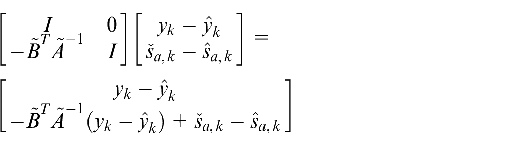
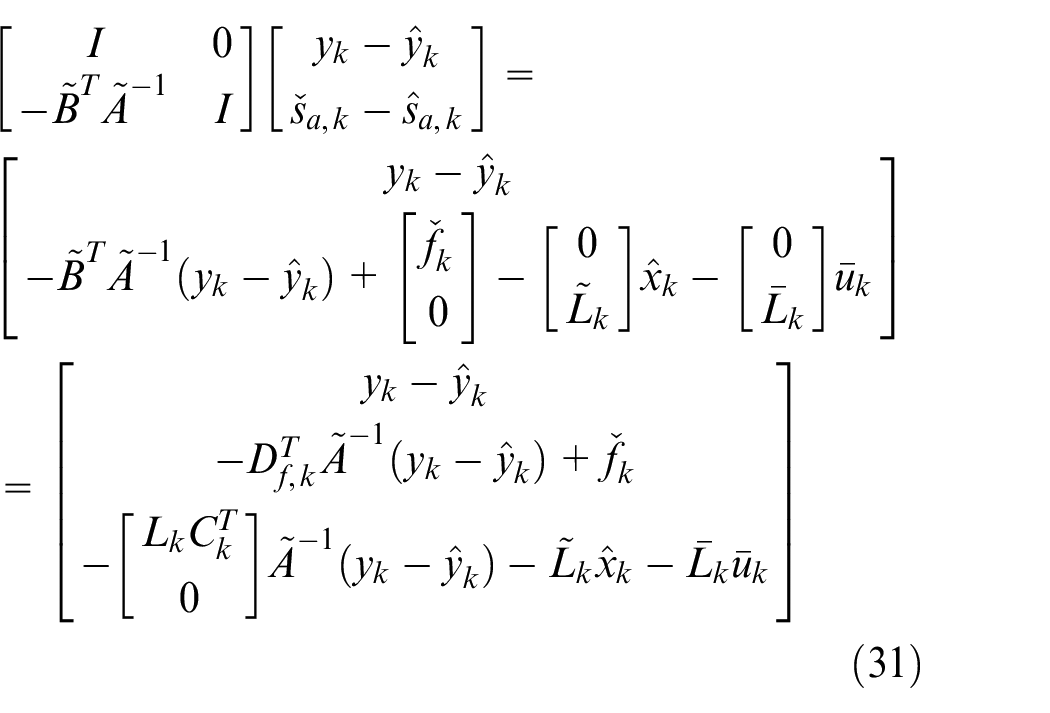
[\begin{matrix} I & 0 \\ - {\tilde{B}}^{T} {\tilde{A}}^{- 1} & I \end{matrix}] [\begin{matrix} y_{k} - {\hat{y}}_{k} \\ {\overset{\lor}{s}}_{a, k} - {\hat{s}}_{a, k} \end{matrix}] = [\begin{matrix} y_{k} - {\hat{y}}_{k} \\ - {\tilde{B}}^{T} {\tilde{A}}^{- 1} (y_{k} - {\hat{y}}_{k}) + {\overset{\lor}{s}}_{a, k} - {\hat{s}}_{a, k} \end{matrix}]

we then have the following relationship from systems (28)–(30)

\begin{matrix} [\begin{matrix} I & 0 \\ - {\tilde{B}}^{T} {\tilde{A}}^{- 1} & I \end{matrix}] [\begin{matrix} y_{k} - {\hat{y}}_{k} \\ {\overset{\lor}{s}}_{a, k} - {\hat{s}}_{a, k} \end{matrix}] = \\ [\begin{matrix} y_{k} - {\hat{y}}_{k} \\ - {\tilde{B}}^{T} {\tilde{A}}^{- 1} (y_{k} - {\hat{y}}_{k}) + [\begin{matrix} {\overset{\lor}{f}}_{k} \\ 0 \end{matrix}] - [\begin{matrix} 0 \\ {\tilde{L}}_{k} \end{matrix}] {\hat{x}}_{k} - [\begin{matrix} 0 \\ {\bar{L}}_{k} \end{matrix}] {\bar{u}}_{k} \end{matrix}] \\ = [\begin{matrix} y_{k} - {\hat{y}}_{k} \\ - D_{f, k}^{T} {\tilde{A}}^{- 1} (y_{k} - {\hat{y}}_{k}) + {\overset{\lor}{f}}_{k} \\ - [\begin{matrix} L_{k} C_{k}^{T} \\ 0 \end{matrix}] {\tilde{A}}^{- 1} (y_{k} - {\hat{y}}_{k}) - {\tilde{L}}_{k} {\hat{x}}_{k} - {\bar{L}}_{k} {\bar{u}}_{k} \end{matrix}] \end{matrix}

(31)

where ${\tilde{L}}_{k} = [\begin{matrix} H_{1, k} \\ 0 \end{matrix}]$ and ${\bar{L}}_{k} = [\begin{matrix} 0 \\ H_{2, k} \end{matrix}]$ .

Recalling the necessary and sufficient condition that ensures the existence of the fault estimator, that is

\tilde{A} > 0, \overset{\lor}{D} < 0

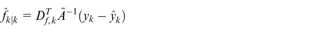
and applying Corollary 2, a natural choice that guarantees $J_{am, k} |_{L_{k} = 0} = J_{m, k} > 0$ through system (31) is

{\overset{\lor}{f}}_{k | k} = D_{f, k}^{T} {\tilde{A}}^{- 1} (y_{k} - {\hat{y}}_{k})

which is system (26). This completes the proof. □

After choosing a suitable ${\overset{\lor}{f}}_{k | k}$ , the final task is to find an algorithm that computes the key intermediate variable ${\hat{x}}_{k}$ . From Hassibi et al.,²⁷ Corollary 2, and Theorem 1, we know that ${\hat{x}}_{k}$ can be computed by the projection of $x_{k}$ on $L {{y_{z, j}}_{j = 0}^{k - 1}}$ in Krein space. Corollary 3 states the evolution of ${\hat{x}}_{k}$ .

Corollary 3

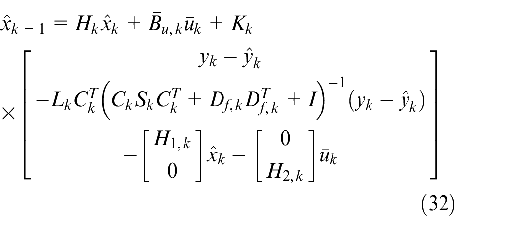
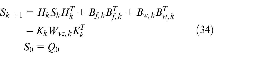
The state variable of the estimator ${\hat{x}}_{k}$ can be computed in the following way

\begin{matrix} {\hat{x}}_{k + 1} = H_{k} {\hat{x}}_{k} + {\bar{B}}_{u, k} {\bar{u}}_{k} + K_{k} \\ \times [\begin{matrix} y_{k} - {\hat{y}}_{k} \\ - L_{k} C_{k}^{T} {(C_{k} S_{k} C_{k}^{T} + D_{f, k} D_{f, k}^{T} + I)}^{- 1} (y_{k} - {\hat{y}}_{k}) \\ - [\begin{matrix} H_{1, k} \\ 0 \end{matrix}] {\hat{x}}_{k} - [\begin{matrix} 0 \\ H_{2, k} \end{matrix}] {\bar{u}}_{k} \end{matrix}] \end{matrix}

(32)

where

K_{k} = (H_{k} S_{k} C_{z, k}^{T} + B_{f, k} D_{f, k}^{T}) W_{yz, k}^{- 1}

(33)

with ${\hat{x}}_{0} = 0$ and

\begin{matrix} S_{k + 1} = H_{k} S_{k} H_{k}^{T} + B_{f, k} B_{f, k}^{T} + B_{w, k} B_{w, k}^{T} \\ - K_{k} W_{yz, k} K_{k}^{T} \\ S_{0} = Q_{0} \end{matrix}

(34)

Proof

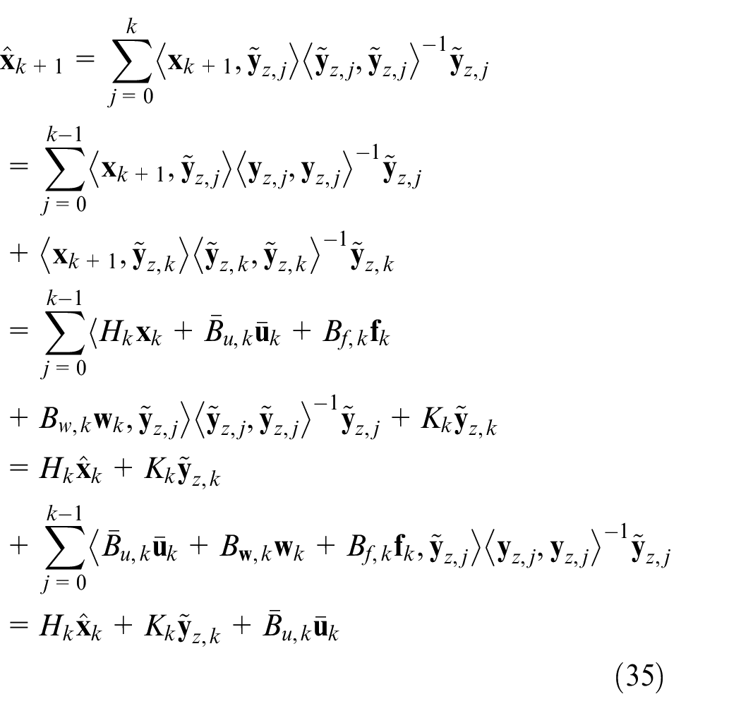
Since ${\hat{x}}_{k}$ can be computed by the projections of $x_{k}$ on $L {{y_{z, j}}_{j = 0}^{k - 1}}$ in Krein space, we immediately have

\begin{matrix} {\hat{x}}_{k + 1} = \sum_{j = 0}^{k} 〈 x_{k + 1}, {\tilde{y}}_{z, j} 〉 {〈 {\tilde{y}}_{z, j}, {\tilde{y}}_{z, j} 〉}^{- 1} {\tilde{y}}_{z, j} \\ = \sum_{j = 0}^{k - 1} 〈 x_{k + 1}, {\tilde{y}}_{z, j} 〉 {〈 y_{z, j}, y_{z, j} 〉}^{- 1} {\tilde{y}}_{z, j} \\ + 〈 x_{k + 1}, {\tilde{y}}_{z, k} 〉 {〈 {\tilde{y}}_{z, k}, {\tilde{y}}_{z, k} 〉}^{- 1} {\tilde{y}}_{z, k} \\ = \sum_{j = 0}^{k - 1} 〈 H_{k} x_{k} + {\bar{B}}_{u, k} {\bar{u}}_{k} + B_{f, k} f_{k} \\ + B_{w, k} w_{k}, {\tilde{y}}_{z, j} 〉 {〈 {\tilde{y}}_{z, j}, {\tilde{y}}_{z, j} 〉}^{- 1} {\tilde{y}}_{z, j} + K_{k} {\tilde{y}}_{z, k} \\ = H_{k} {\hat{x}}_{k} + K_{k} {\tilde{y}}_{z, k} \\ + \sum_{j = 0}^{k - 1} 〈 {\bar{B}}_{u, k} {\bar{u}}_{k} + B_{w, k} w_{k} + B_{f, k} f_{k}, {\tilde{y}}_{z, j} 〉 {〈 y_{z, j}, y_{z, j} 〉}^{- 1} {\tilde{y}}_{z, j} \\ = H_{k} {\hat{x}}_{k} + K_{k} {\tilde{y}}_{z, k} + {\bar{B}}_{u, k} {\bar{u}}_{k} \end{matrix}

(35)

where

\begin{matrix} 〈 x_{k + 1}, {\tilde{y}}_{z, j} 〉 = 〈 H_{k} x_{k} + {\bar{B}}_{u, k} {\bar{u}}_{k} + B_{f, k} f_{k} + B_{w, k} w_{k}, {\tilde{y}}_{z, j} 〉 \\ = 〈 H_{k} x_{k} + {\bar{B}}_{u, k} {\bar{u}}_{k} + B_{f, k} f_{k} + B_{w, k} w_{k}, C_{z, k} e_{k} + D_{f, k} f_{k} + v_{z, k} 〉 \\ = H_{k} S_{k} C_{z, k}^{T} + B_{f, k} D_{f, k}^{T} \end{matrix}

(36)

Thus, systems (35) and (36) lead to the form of the filter in system (32) with its gain matrix in system (33).

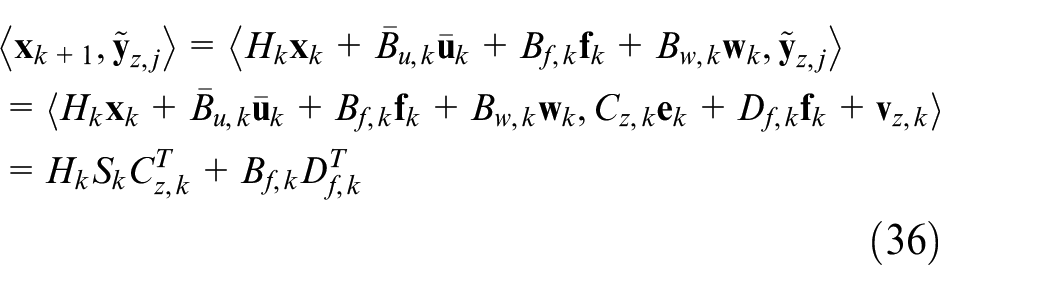
Note that the variables $X_{k} = 〈 x_{k}, x_{k} 〉$ and $P_{k} = 〈 {\hat{x}}_{k}, {\hat{x}}_{k} 〉$ can be directly computed based on the Krein space model (19) using the inner product as follows, respectively

\begin{matrix} X_{k + 1} = H_{k} X_{k} H_{k}^{T} + {\bar{B}}_{u, k} {\bar{u}}_{k} {\bar{u}}_{k}^{T} {\bar{B}}_{u, k}^{T} + B_{f, k} B_{f, k}^{T} \\ + B_{w, k} B_{w, k}^{T} \\ X_{0} = Q_{0} \end{matrix}

and

\begin{matrix} P_{k + 1} = H_{k} P_{k} H_{k}^{T} + {\bar{B}}_{u, k} {\bar{u}}_{k} {\bar{u}}_{k}^{T} {\bar{B}}_{u, k}^{T} \\ + K_{k} 〈 {\tilde{y}}_{z, k}, {\tilde{y}}_{z, k}^{T} 〉 K_{k}^{T} \\ P_{0} = 0 \end{matrix}

Hence, by using the orthogonal property between ${\hat{x}}_{k}$ and $e_{k}$ , we have $S_{k} = X_{k} - P_{k}$ , which is system (34). This completes the proof. □

Remarks

Before ending the main body of this study, we would like to give some remarks:

In view of Theorem 1 and Corollary 3, our proposed algorithm provides a generalized form on some kinds of discrete time-variant systems, such as nonlinear system with differentiable condition, linear nominal systems, and uncertain linear system. It should be pointed out that, although one can neglect the linearization errors when using Taylor series expansions for the considered nonlinear system, or directly augment these errors into unknown input, some design conservatism may be introduced by artificially ignoring some prior information on the system. In contrast, our algorithm does not produce the conservatism by taking these errors in the design procedure.³⁰

In this study, the considered nonlinearity only appears in the state equation (1). We would like to mention that, our result can also be extended to the cases when the same category of the nonlinearity occurs in the measurement equation by choosing appropriate auxiliary variables and the corresponding dynamic model in Krein space.

Due to the recursive property of the proposed algorithm, the fault signal can be estimated in real time. For nonlinear systems subject to stochastic modeling uncertainties, unreliable communication links, or with other kinds of random properties, much effort should be paid on online fault detection, fault estimation, and fault isolation, which leads to our future work.

An illustrative example

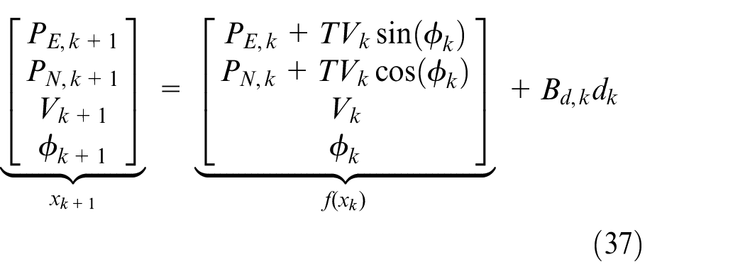
In recent years, indoor robot localization has attracted wide attention. In order to acquire the accurate position information, some state estimators such as Kalman filter and finite impulse response filter are used as the data fusion filter to improve the accuracy.³¹ The state equation used by these filters at time index $k$ can be described as follows

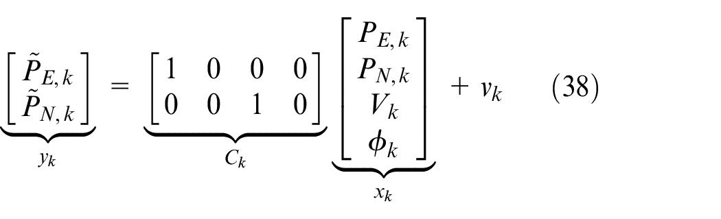
\underset{x_{k + 1}}{\underset{︸}{[\begin{matrix} P_{E, k + 1} \\ P_{N, k + 1} \\ V_{k + 1} \\ ϕ_{k + 1} \end{matrix}]}} = \underset{f (x_{k})}{\underset{︸}{[\begin{matrix} P_{E, k} + T V_{k} \sin (ϕ_{k}) \\ P_{N, k} + T V_{k} \cos (ϕ_{k}) \\ V_{k} \\ ϕ_{k} \end{matrix}]}} + B_{d, k} d_{k}

(37)

here, $T$ is the sampling interval, and the state variables can be represented using a vector as $x_{k} = [\begin{matrix} P_{E, k} & P_{N, k} & \begin{matrix} V_{k} & ϕ_{k} \end{matrix} \end{matrix}]^{T}$ , where $P_{E, k}$ and $P_{N, k}$ , respectively, denote the robot position in the east and north directions. $V_{k}$ denotes the robot velocity, and $ϕ_{k}$ is the yaw angle of robot. $d_{k}$ means the process disturbance with coefficient matrix $B_{d, k}$ . The observation output equation at time index $k$ can be described as follows

\underset{y_{k}}{\underset{︸}{[\begin{matrix} {\tilde{P}}_{E, k} \\ {\tilde{P}}_{N, k} \end{matrix}]}} = \underset{C_{k}}{\underset{︸}{[\begin{matrix} 1 & 0 & 0 & 0 \\ 0 & 0 & 1 & 0 \end{matrix}]}} \underset{x_{k}}{\underset{︸}{[\begin{matrix} P_{E, k} \\ P_{N, k} \\ V_{k} \\ ϕ_{k} \end{matrix}]}} + v_{k}

(38)

where $y_{k}$ is the measurement vector and $v_{k}$ is the measurement noise. ${\tilde{P}}_{E, k}$ and ${\tilde{P}}_{N, k}$ are the ultra wideband (UWB)-derived positions in the east and north directions, respectively. $v_{k}$ represents the measurement noise.

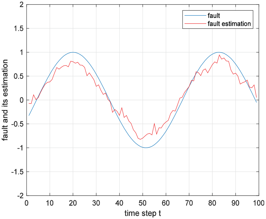
Based on the above state-space models, that is, systems (37) and (38), consider the circumstance that when process fault and/or sensor fault occurs, the simulation of fault estimation for indoor robot localization systems is performed. During the simulation, the sampling time $T$ is set to 0.01 s. The process disturbance $d$ and measurement noise $v$ are assumed to be zero-mean white noise sequences with covariance matrices $0.01 I$ and $0.0225 I$ , respectively. The fault signal is simulated as

f_{k} = \cos (0.1 (k - 20))

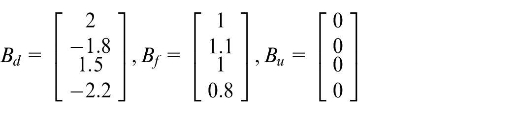
and the related matrices in system (1) are assumed to be as follows

B_{d} = [\begin{matrix} 2 \\ - 1.8 \\ \begin{matrix} 1.5 \\ - 2.2 \end{matrix} \end{matrix}], B_{f} = [\begin{matrix} 1 \\ 1.1 \\ \begin{matrix} 1 \\ 0.8 \end{matrix} \end{matrix}], B_{u} = [\begin{matrix} 0 \\ 0 \\ \begin{matrix} 0 \\ 0 \end{matrix} \end{matrix}]

Let $γ = 1.2$ , $A_{k} = 0.3 I$ , $L_{k} = 0.1 I$ , and $Q_{O} = 100 I$ , by using Theorem 1 and Corollary 3, the estimated signal ${\overset{\lor}{f}}_{k | k}$ can be generated. Figure 1 shows ${\overset{\lor}{f}}_{k | k}$ along with $f_{k}$ . Based on the simulation results, we know that the proposed algorithm can track the fault well for the concerned nonlinear time-variant systems.

Figure 1.

Fault signal and its estimation.

Conclusion

In this paper, the fault estimation problem for a class of time-variant nonlinear systems has been studied in the $H_{\infty}$ setting, where the concerned nonlinearity is assumed to be continuously differentiable. By employing the Taylor series expansions, the original nonlinear system has been rewritten as a LTV system with modeling errors. An alternative system and its corresponding indefinite quadratic performance function have been addressed in lieu of the uncertain dynamics and the traditional performance index, respectively. After formulating the estimation issue as a two-stage optimization problem, an auxiliary model in Krein space has been introduced. The well-known orthogonal projection technique has been applied to solve this optimization problem, and a necessary and sufficient condition on the existence of the fault estimator has been obtained. To achieve real-time fault estimation, a recursive algorithm for calculating the gain matrix of the estimator has been provided, where its effectiveness has been verified by applying the proposed method to a faulty indoor robot localization system.

Footnotes

Declaration of conflicting interests

The author(s) declared no potential conflicts of interest with respect to the research, authorship, and/or publication of this article.

Funding

The author(s) disclosed receipt of the following financial support for the research, authorship, and/or publication of this article: This work was supported in part by the National Natural Science Foundation of China under grant numbers 61973135, 91948201, 61773242, and 61673245; the Shandong Provincial Key R&D Program, China, under grant no. 2018GGX104025; and the project ZR2017QF007 supported by Shandong Provincial Natural Science Foundation.

ORCID iD

Yueyang Li

References

Blanke

Kinnaert

Lunze

, et al. Diagnosis and fault-tolerant control, vol. 2. Berlin: Springer, 2006.

Ding

SX.

Model-based fault diagnosis techniques: design schemes, algorithms, and tools. Berlin; Heidelberg: Springer, 2008.

Zaytoon

Lafortune

Overview of fault diagnosis methods for discrete event systems. Ann Rev Contr 2013; 37(2): 308–320.

Zhong

Xue

Ding

SX.

A survey on model-based fault diagnosis for linear discrete time-varying systems. Neurocomputing 2018; 306: 51–60.

Karimi

Zhong

, et al. Fault detection for linear discrete time-varying systems with multiplicative noise: the finite-horizon case. IEEE Trans Cir Syst I Reg 2018; 65(10): 3492–3505.

Karimi

Ahn

, et al. Optimal residual generation for fault detection in linear discrete time-varying systems with uncertain observations. J Franklin Inst 2018; 355(7): 3330–3353.

Guo

Optimal fault-detection filtering for non-Gaussian systems via output PDFs. IEEE Trans Syst Man Cybernet A Syst Human 2009; 39(2): 476–481.

Wang

Shi

Lim

CC.

H_–/H_∞ fault detection observer in finite frequency domain for linear parameter varying descriptor systems. Automatica 2017; 86: 38–45.

Long

Park

Transmission-dependent fault detection and isolation strategy for networked systems under finite capacity channels. IEEE Trans Cybernet 2017; 47(8): 2266–2278.

10.

Zhou

KM.

A time domain approach to robust fault detection of linear time-varying systems. Automatica 2009; 45(1): 94–102.

11.

Zhong

Ding

Zhou

DH.

A new scheme of fault detection for linear discrete time-varying systems. IEEE Trans Automat Contr 2016; 61(9): 2597–2602.

12.

Pertew

Marquez

Zhao

LMI-based sensor fault diagnosis for nonlinear Lipschitz systems. Automatica 2007; 43(8): 1464–1469.

13.

Zhang

Polycarpou

Parisini

Fault diagnosis of a class of nonlinear uncertain systems with Lipschitz nonlinearities using adaptive estimation. Automatica 2010; 46(2): 290–299.

14.

Polycarpou

Trunov

AB.

Learning approach to nonlinear fault diagnosis: detectability analysis. IEEE Trans Automat Contr 2000; 45(4): 806–812.

15.

Chen

, et al. Event triggered fault detection of nonlinear networked systems. IEEE Trans Cybernet 2017; 47(4): 1041–1052.

16.

Liu

Shi

, et al. Fault detection filtering for nonlinear switched systems via event-triggered communication approach. Automatica 2019; 101: 365–376.

17.

Persis

Isidori

A geometric approach to nonlinear fault detection and isolation. IEEE Trans Automat Contr 2002; 46(6): 853–865.

18.

Wang

Shu

, et al. H_∞ fault estimation with randomly occurring uncertainties, quantization effects and successive packet dropouts: the finite-horizon case. Int J Robust Nonlin Contr 2015; 25(15): 2671–2686.

19.

Dong

Wang

Ding

, et al. On H_∞ estimation of randomly occurring faults for a class of nonlinear time-varying systems with fading channels. IEEE Trans Automat Contr 2016; 61(2): 479–484.

20.

Ren

Wang

Yang

Fault estimation for time-varying Markovian jump systems with randomly occurring nonlinearities and time delays. J Franklin Inst 2016; 354(3): 1388–1402.

21.

Chao

Sheng

Liu

, et al. Event-based H_∞ fault estimation for networked time-varying systems with randomly occurring nonlinearities and (x, v)-dependent noises. Neurocomputing 2018; 285: 220–229.

22.

Dong

Wang

, et al. Non-fragile distributed fault estimation for a class of nonlinear time-varying systems over sensor networks: the finite-horizon case. IEEE Trans Sig Inform Process Netw 2019; 5(1): 61–69.

23.

Dong

Hou

Wang

, et al. Finite-horizon fault estimation under imperfect measurements and stochastic communication protocol: dealing with finite-time boundedness. Int J Robust Nonlin Contr 2019; 29: 117–134.

24.

Liu

Zhong

Liu

A new residual evaluation function based fault diagnosis for a kind of nonlinear systems. Asian J Contr 2019; 21(4): 1–13.

25.

Calafiore

Reliable localization using set-valued nonlinear filters. IEEE Trans Syst Man Cybernet A Syst Human 2005; 35(2): 189–197.

26.

Wang

Gao

, et al. Extended Kalman filtering with stochastic nonlinearities and multiple missing measurements. Automatica 2012; 48(9): 2007–2015.

27.

Hassibi

Sayed

Kailath

Indefinite-quadratic estimation and control: a unified approach to H₂ and H_∞ theories, vol. 16. Philadelphia, PA: SIAM, 1999.

28.

Zhao

Ding

Wang

, et al. Krein-space based robust H_∞ fault estimation for two-dimensional uncertain linear discrete time-varying systems. Syst Contr Lett 2018; 115: 41–47.

29.

Zhao

Ding

Karimi

, et al. Robust H-infinity filtering for two-dimensional uncertain linear discrete time-varying systems: a Krein space-based method. IEEE Trans Automat Contr. Epub ahead of print 2 April 2019. DOI: 10.1109/TAC.2019.2908699.

30.

Jin

Park

Set-valued estimation approach to recursive robust H_∞ filtering. IEE Proc Contr Theor Appl 2004; 151(9): 773–782.

31.

Karimi

, et al. Real-time accurate pedestrian tracking using extended finite impulse response filter bank for tightly coupling recent inertial navigation system and ultra-wideband measurements. Proc IMechE, Part I: J Systems and Control Engineering 2018; 232(4): 464–472.

Fault estimation for a class of nonlinear time-variant systems through a Krein space–based approach

Abstract

Keywords

Introduction

Notations

Problem formulation

Lemma 1

Proof

Corollary 1

Problem 1

Main results

Corollary 2

Theorem 1

Proof

Corollary 3

Proof

Remarks

An illustrative example

Conclusion

Footnotes

Declaration of conflicting interests

Funding

ORCID iD

References