National patterns of income and wealth inequality

Abstract

The aim of this article is to show that wealth must be treated as a distinct dimension of social stratification alongside income. In a first step, we explain why social stratification researchers have largely overlooked wealth in the past and present a detailed definition of wealth by differentiating it from income. In the empirical part of the article, we analyze the distribution of wealth across 18 countries, and we describe and compare national patterns of wealth inequality to those of income inequality making use of different data sources. Our results show – first – that there is strong variation in the distribution of wealth between these 18 countries, and – second – that levels of wealth inequality significantly differ from levels of income inequality in about half of the countries analyzed. Surprisingly high levels of wealth inequality we find in Sweden and Denmark, two countries widely considered being highly egalitarian societies. Conversely, the Southern European countries – where income inequality is relatively high – exhibit comparatively low levels of wealth inequality.

Keywords

Income inequality net worth social inequality social stratification wealth inequality

Introduction

International comparative research on social inequality shows that modern societies exhibit very different and distinct patterns of social inequality, with its level and persistency depending strongly on national institutional settings. Most studies within this field, however, consider social inequalities fundamentally in terms of inequalities deriving from the labor market (especially in terms of income inequality), while neglecting the relevance of wealth in the stratification process. Especially during phases of economic insecurity, such as illness or retirement, wealth is of great importance to stabilize consumption, in particular in less generous welfare states. Studying wealth becomes even more relevant when we consider how intergenerational transfers serve as powerful social mechanisms that can reproduce and intensify existing social inequalities. Moreover, given the aging of industrialized societies, along with the growing importance of private savings in the course of the most recent pension reforms all over Europe, wealth will probably serve as a crucial source of individuals’ well-being in modern societies (cf. Davies and Shorrocks, 2000: 608). The few empirical studies conducted until now which analyze the relationship between income and wealth were able to show that the correlation between the two measures is much weaker than one might expect, ranging from 0.3 to 0.5 (e.g. Keister and Moeller, 2000; Wolff, 2006). Moreover, wealth has been found to affect various social outcomes like education, occupation, health, or well-being, even after controlling for income (Bonini, 2007; Meer et al., 2003; Pfeffer and Hällsten, 2014), indicating its social stratification effects. Thus, it is reasonable to assume that studies addressing only income are likely to paint a one-sided or even inaccurate picture of economic and, in a broader sense, social inequalities.

With this article, we intend to contribute to a broader understanding of social inequality by going beyond inequalities derived from the labor market and drawing attention to wealth as an important but often neglected variable – both on a conceptual and methodological level – in social stratification research (cf. Piketty, 2014). In a first step, we explain why social stratification researchers have largely overlooked wealth in the past. Moreover, we formulate theoretical arguments as to why wealth must be treated as a distinct dimension of social stratification alongside income. In this context, we also present a detailed definition of wealth by differentiating it from income. In the empirical part of the article, we analyze the distribution of wealth, and we describe and compare national patterns of wealth inequality to those of income inequality. We apply hierarchical cluster methods to find clusters of countries with similar levels of wealth and income inequality. The aim of this article is, first, to find out how private wealth is distributed in different countries and, second, to find out if national patterns of wealth inequality resemble those of income inequality. This article shall be understood as a descriptive introduction to the topic of cross-national wealth studies within the framework of social stratification research.

For our descriptive analyses, we make use of a number of different data sources: the Survey of Health, Ageing and Retirement in Europe (SHARE), Organisation for Economic Co-operation and Development (OECD) income data, and the wealth data provided by the Global Wealth Databooks (GWD) (Credit Suisse Research Institute, 2010, 2011, 2012, 2013). We compare income and wealth holdings across 17 European countries and one country from the Middle East (Israel).

The longtime disregard of wealth in social stratification research

Despite the relevance of wealth for the process of social stratification, serious research on wealth has, for a very long time, almost exclusively been conducted in the field of economics (Atkinson, 1971; Davies and Shorrocks, 2000; Wolff, 2006). We attribute this oversight to both substantive and empirical factors.

At the end of the Second World War, the ownership and accumulation of wealth was still the preserve of elite groups in society. Consequently, wealth was mainly understood in terms of power, and wealth research was assigned to the field of elite sociology (e.g. Le Bon, 1939; Michels, 1925; Mosca, 1950: cf. Spilerman, 2000). Only thereafter, in times of economic prosperity, political stability, and peace in the industrialized countries, did wealth become a quantitatively significant economic resource for the population as a whole. Nevertheless, social stratification research tends to be overly focused on inequalities deriving solely from the labor market (occupational status and/or earnings), while neglecting the relevance of wealth in the stratification process.

Functionalist theories of social stratification understand societies as operating on meritocratic principles, and consider wealth only if it is self-generated (life-cycle wealth). Transferred wealth contradicts the principles of equal opportunity and merit, and is not taken into account. Theories of social class are oriented toward labor market processes, with a strong focus on the individual actor. Their main interest is the organization of work in modern industrial societies. Accordingly, wealth is discussed only peripherally. Marx’ concept of class (see, for example, Grusky, 2008: 74–90) is derived directly from the individual’s position in the production system. Yet, in addition to the two main classes in capitalism – the proletariat and the bourgeoisie – Marx also mentioned the petty bourgeoisie and landowners, whose social position is based on their ownership of means of production. In later approaches, such as in the work of Bourdieu (1984, 1986), Dahrendorf (1959) and Durkheim (2008), the concept of class is extended, and wealth is considered more explicitly. Weber’s (1922) class concept provides the most explicit discussion of wealth; he understands the ownership of property as representing the main difference between classes. Weber differentiates between the property class – consisting of entrepreneurs (who use their wealth in commercial ventures) and rentiers (who profit by interest on their property) – and the property-less class, defined by the kinds of services they provide in the labor market.

Since the 1980s, theories of social environments (milieus) and lifestyles have tried to offer a holistic approach to the explanation of social life and continue to emphasize the multidimensionality of social inequality. They deny that one’s occupational position is the single most important feature in the definition of social class, resulting in a change of perspective from the individual actor to the family as the most important unit in the process of social stratification. Social stratification is no longer understood as a state, but as a process that develops over the life course, and is subject to changes. As the accumulation of wealth is such a process, unfolding over the whole life course, it can be best approached by adopting a life course perspective (Elder, 1975; Kohli, 1986; Mayer and Müller, 1986). The process of wealth accumulation is strongly related to and interdependent on important life course events (e.g. marriage, divorce, childbirth, death of the spouse) and other life course processes (e.g. occupational or family trajectories). Unfortunately, even now there is a lack of suitable data to enable an empirical analysis of these interdependent processes, trajectories and events, which brings us to the empirical reasons for the longtime disregard of wealth in social stratification research.

The first wealth survey to have been conducted was in the United States in the 1960s (when the already established ‘Survey of Financial Characteristics of Consumers’ added a wealth module). A number of similar studies in the United States were to follow, but not until 1980; in other industrialized countries, wealth studies such as these only appeared as late as the 1990s and 2000s. In addition, a number of cross-national wealth surveys (e.g. the Luxembourg Wealth Study (LWS), the Household Finance and Consumption Survey (HFCS) and the Survey of Health, Ageing and Retirement (SHARE)) have started recently. Nevertheless, many surveys cover only relatively short periods, so they allow us to study the accumulation of wealth from a ‘real’ life course perspective only in some years.

In recent years, however, sociologists have become interested in studying wealth (e.g. Elmelech, 2008; Keister and Moeller, 2000; Semyonov and Lewin-Epstein, 2011; Spilerman, 2000). The increasing relevance of wealth in social stratification research is likely to be related to some more recent social and political developments. The first is population aging and the accompanying public pension retirement limit set by the modern welfare states. These factors turned old age into a distinct phase of life. This life stage is much less structured by labor market activity, while leisure and consumption become increasingly important (Kohli, 1988). Thus, as individuals grow older, wealth increasingly determines their economic status, while income becomes less meaningful. The second reason is the increasing importance of private provision for old age. As a reaction to population aging, welfare states nowadays reduce public pension benefits and try to set incentives for private provision for old age. Responsibility for old-age provision is increasingly being transferred from the welfare state to the individual actor, which makes the accumulation of private wealth an even more relevant topic for the overall population.

Wealth and income – Definitional issues

While both income and wealth are important features of individual economic standing, each has different properties. Income, generally understood to be earned income, is a flow measure that represents a snapshot of an economic entity’s financial situation at a certain point in time, or over a minor interval (usually a week, month, or year). It can vary considerably from one period to the next and is restricted to persons or households who actively engage in the labor force (earned income), or who were engaged in the labor force at some time in the past (transferred income). In contrast, wealth is a stock measure, which – originating from a certain value – increases by inflows and decreases by outflows. Stock measures feature the following distinct characteristics: they represent the state of a system and are thus the basis for decision-making, they bring inertia, history and memory to the system by accumulating events of the past, and they allow delays and enable dynamic imbalances between inflows and outflows (Forrester, 1961, 1968). In this regard, the economic unit of a person or household can be understood as a system. Accumulated assets represent the system’s material condition. Based on these assets, the economic unit will make decisions regarding, for example, consumption and investment. Larger short-term changes in the stock of wealth are possible, for example, through inheritances or poor investments. These changes are, however, infrequent events often correlating with decisive life changes (like the death of one’s parents). As such, the stock of wealth accumulated represents resources of the individual’s past, present, and future (potential) financial well-being (Cowell et al., 2012). Correspondingly, Spilerman (2000) understands wealth as an individual’s or household’s consumption potential, or more precisely, its capacity to maintain a particular standard of living.

In addition, the process of wealth accumulation is a typical process of cumulative advantage (DiPrete and Eirich, 2006). Once a certain amount of wealth is accumulated, it will replicate itself through the mechanism of compound interest. At the same time, the state of having no or only low wealth is likely to be persistent over time. This is one important reason why the distribution of wealth is likely to be more unequal than the distribution of income. Over and above, this is related to the fact that compared to the distribution of income, the distribution of wealth is much more likely to show extreme outliers on the top of the distribution. Various scholars argue that in the United States, for example, the top 1 percent of the wealth distribution holds nearly 50 percent of total wealth (Davies et al., 2009; Wolff, 2002).

Finally, the functions of wealth are much broader than those of income, which can be either saved (or invested) or consumed. Frick and Grabka (2009b: 579) name seven functions of wealth. As already stated above, wealth has the characteristic of replicating itself through the mechanism of compound interest, resulting in the generation of further income (income function). Non-financial assets such as property, vehicles, or art all share the function of utility, be it in the form of recreation, greater independence, or other direct benefits (utility function). In the case of an expected or unexpected decrease or loss of income, wealth can serve to stabilize consumption (security function). Wealth can also provide access to political power (power function), and it can be used to achieve or maintain high levels of social status (social status maintenance function). In addition, wealth can serve to finance the education of one’s children or grandchildren (socialization function), and – perhaps most importantly – wealth can be transferred over generations (inheritance function) and might thus serve as a powerful social mechanism to reproduce or intensify existing social inequalities.

According to Meade (1964, 1975), the wealth of an economic entity at a certain time is determined by age and the history of earnings (starting with birth), saving rates (or consumption rates), and rates of return plus inheritances and gifts. Total wealth can thus be decomposed into two components: self-accumulated wealth (life-cycle wealth) and transferred wealth (via inter vivos transfer or bequests) (Davies and Shorrocks, 2000; Gale and Scholz, 1994). In order to analyze and understand wealth inequalities, it is crucial to know whether most of the accumulated wealth holdings stem from saved income or from transferred wealth. This question is, however, very difficult to answer, as one would need detailed longitudinal information about personal income and wealth for at least two consecutive generations, which is not widely available, if at all.

For the Unites States, however, many studies exist which either directly estimate the contribution of life-cycle wealth to total wealth, simulate the bequeathing behavior of overlapping generations, or measure transferred wealth via surveys that directly ask respondents about the percentage of total wealth they received through transfers (Gale and Scholz, 1994). Results from the first and second types of studies are very heterogeneous with estimates of the contribution of transferred wealth to total wealth ranging from less than 20 percent (Modigliani, 1988a, 1988b) to approximately 80 percent (Kotlikoff and Summers, 1981; White, 1978). Survey studies are more consistent, and estimate the contribution of transferred wealth to total wealth at around 20 percent (Gale and Scholz, 1994; Modigliani, 1988a; Wolff and Gittleman, 2014). A severe problem for all three types of research is that bequests need not to be intended, but can be accidental (Gale and Scholz, 1994). For this reason, Kessler and Masson (1989) even state that that it is ‘virtually impossible to distinguish life-cycle from bequest savings’ (p. 145). Obviously, the contribution of transferred wealth to total wealth is far from clear.

Considering the unique characteristics and the numerous functions of wealth – as compared to income – differences in levels of wealth and levels of wealth inequality are likely to be more consequential in terms of social stratification. Social stratification becomes social inequality if access to social positions or social goods is unequal and if these positions or goods are systematically related to advantageous or disadvantageous conditions of acting and living (cf. Solga et al., 2009: 15). As already explained, due to its specific characteristics, the distribution of wealth is likely to be more unequal than the distribution of income, which has been empirically confirmed by a number of studies (Davies et al., 2008; Davies and Shorrocks, 2000; Frick and Grabka, 2009a). There are numerous studies which analyze the relationship between wealth and educational or occupational outcomes (Filmer and Pritchett, 2004; Nam and Huang, 2009; Pfeffer and Hällsten, 2014), between wealth and health or mortality (Attanasio and Hoynes, 2000; Meer et al., 2003; Semyonov et al., 2013) or between wealth and well-being (Bonini, 2007; Headey et al., 2008; Hochman and Skopek, 2013). These studies all try to establish whether differences in levels of wealth or levels in wealth inequality imply the same stratification consequences as differences in levels of income and income inequality, and if these effects persist even after controlling for income. A positive relationship has been found, for example, between wealth and education: Nam and Huang (2009) report a positive effect of parents’ financial situation on their children’s educational attainment in the Unites States, and Pfeffer and Hällsten (2014) find even more evidence for an intergenerational transmission of advantage through wealth. Controlling for parental income, the authors find children from wealthier families perform better in life in the United States, Germany, and Sweden. In Germany and Sweden, children from wealthier families show higher educational outcomes compared to children from less wealthy families. In the United States, parental wealth also has a positive effect on occupational status and income. In addition to that, the authors report that in all three countries, parental wealth impedes downward social mobility while at the same time increasing the chances for upward social mobility. Finally, wealth and health have also been found to be positively related. Moreover, wealth has been found to affect different dimensions of subjective well-being (quality of life, life satisfaction, depression), even when controlling for income. This indicates that wealth might not only be a distinct dimension of social stratification, but also of social inequality. We therefore argue that, for a comprehensive understanding of economic and social stratification, it is crucial that we go beyond inequalities derived from the labor market by also studying the distribution of private wealth.

National differences in the distributions of wealth and income

The main motivation of this article is to give the reader an initial idea of the distribution of private wealth across countries and to enable a comparison to the distribution of income. We do not aim to explain national differences in the distribution of wealth. However, in the following, we will suggest and discuss a number of possible factors that could explain national differences in the distribution of private wealth.

Undoubtedly, individual and household characteristics strongly influence the process of wealth accumulation. Although the contribution of transferred wealth to total wealth is far from clear, it is plausible that earnings differences within and across countries translate into wealth differences to at least some degree. Empirical research reveals that income and wealth show only medium levels of correlation, and that in some countries the level of income inequality significantly deviates from the level of wealth inequality. In line with these findings, Cowell et al. (2013) assert that there are various reasons why levels of income and wealth inequality might differ from each other within countries, and why the distribution of wealth might vary across countries. First, they mention differences in the distribution of individual demographic and economic characteristics across countries as an important part of the explanation for national differences in levels of wealth and wealth inequality. These can be age differences (see also the life-cycle hypothesis of Modigliani and Brumberg, 1954, on the relationship between wealth and age), but also education, race, and marital status, which are found to be important micro-level determinants of national differences in private wealth (Conley, 2009; Henretta and Campbell, 1978; Keister and Moeller, 2000; Oliver and Shapiro, 1990; Semyonov and Lewin-Epstein, 2013). In addition to these demographic variables, a growing number of scholars agree on the importance of psychological variables to complement them (Feldstein, 1995; Furnham, 1985; Thaler, 1990, 1994). Among these variables are self-control, taste for saving, voting patterns, or other preference parameters like the degree of risk aversion.

Second, a number of macro-level factors are likely to affect the distribution of private wealth. Cowell et al. (2013) suggest that both institutional settings and economic environments will affect households’ saving motives and propensities. The standard life-cycle model developed by Modigliani and Brumberg (1954) is a powerful and flexible theoretical framework for explaining individual saving behavior, resulting in national differences in the distribution of wealth via differences in institutional settings. According to this model, saving behavior is the result of an optimization problem of inter-temporal consumption: Perfectly rational and forward-looking actors are faced with a deterministic income path with low earnings at the beginning of their career that increase over their working life and drop to zero when they retire. Trying to keep their marginal utility of consumption constant over time, they borrow at younger ages, save as their earnings increase, and ‘dis-save’ in retirement. In the basic model, neither there are capital market imperfections nor is there uncertainty (e.g. earnings insecurity or uncertainty about the date of death). Saving is understood as earnings minus consumption. The only motivation for saving is provision for old age, and there are no bequests. Individuals work as long as they are able. In this situation, the introduction of a pay-as-you-go public pension system would consequently lead to a perfect substitution between public pension wealth and private savings.

However, based on the findings of Cagan (1965) and Katona (1964), Feldstein (1974) argues that this only holds true for workers who planned to retire close to the official retirement age anyway. For workers who planned to retire later than that, the introduction of an official retirement age would generally induce them to retire earlier than they actually planned, since this will lengthen their total period in retirement. The introduction of a pay-as-you-go public pension system could motivate these workers to increase their savings. Thus, the implementation of a pay-as-you-go public pension system¹ could also have a positive effect on the level of private savings, possibly offsetting the negative one. Either way, the standard life-cycle model suggests that cross-country differences in public pension systems are a powerful explanation of international differences in the distribution of wealth. In an early time-series analysis, in fact, Feldstein (1974) found a strong negative relationship between social security (pension wealth) and aggregate capital accumulation. However, other time-series analyses found this relationship to be much weaker or even non-existent (Barro, 1978; Leimer and Lesnoy, 1982).

Bringing transferred wealth back into the discussion, Cowell et al. (2013) further discuss national differences in the importance of past inheritances, and national differences in the population’s age composition and household structure as representing possible explanatory factors for national differences in the distribution of wealth. In addition, national differences in the taxation of wealth (life-cycle wealth as well as transferred wealth), but also earnings, are likely to have an impact on national differences in the distribution of wealth. Various researchers suggest to further account for differences in financial literacy as an important determinant of saving behavior across, but also within, countries (Bernheim, 1998; Van Rooij et al., 2012). Differences in financial literacy might explain part of the finding that it is usually the highly educated/high-income households, which show a saving profile close to the assumptions of the standard life-cycle model, while the less educated/low-income households hardly save at all. In an international comparative study, Lusardi and Mitchell (2011) found financial literacy scores to be relatively high for individuals in Sweden and the Netherlands, but comparatively low for individuals in Italy and Russia. Similarly, Jappelli (2010) finds financial literacy to be high in Sweden, the Netherlands and Denmark, and low in Italy, Spain, and Poland.

Finally, Cowell et al. (2013) mention nationally specific cultural and historical factors that shape preferences for holding specific types of assets (for example, real estate or stocks and shares) as an explanation for national differences in the distribution of wealth. In line with this argument, Feldstein (1995: 411) suggests the Europeans’ shared experience of inflation and war as an explanation for the higher saving rates in the European population as compared to the United States,² despite the greater generosity of social security retirement programs in Europe. Lusardi and Mitchell (2011) also claim that international differences in financial literacy can be the result of specific historical factors. They found, for example, that individuals in countries with recent experience of inflation scored higher on questions about inflation, and individuals in countries that experienced pension privatization scored higher on questions about risk diversification.

Summing up, in their empirical analyses, Cowell et al. (2013) find that the largest share of national differences in the distribution of wealth cannot be traced back to differences in the distribution of individual characteristics, but rather to national effects, which they could, however, not explain in their analyses due to their small sample size.³ As suggested, and in line with other studies, they find relative levels of income and wealth inequality to be similar in some countries (e.g. the United States), while they strongly differ in others (e.g. Sweden). The following analyses contribute to the research on national differences in the distribution of private wealth. We will describe the distribution of wealth and compare national patterns of wealth inequality to those of income inequality. Therefore, before we present our analyses, we shall briefly trace national patterns of income inequality as detected by past research.

The OECD (2008) publication ‘Growing unequal’ provides an overview of income distributions in OECD countries over the period from the mid-1980s until the mid-2000s. It distinguishes five groups of countries. Denmark and Sweden belong to the ‘low inequality group’, with Gini coefficients for income below 0.3. The ‘below average inequality group’ exhibits Gini coefficients for income that are slightly below the OECD average, which is just above 0.3. Countries belonging to this group are Austria, Australia, Belgium, the Czech Republic, Finland, France, Germany, Hungary, Luxembourg, the Netherlands, Norway, the Slovak Republic, and Switzerland. This group is followed by the ‘above average inequality group’ that is composed of Korea, Canada, Spain, Japan, Greece, Ireland, New Zealand, and the United Kingdom. The fourth group is the ‘high inequality group’, consisting of Italy, Poland, the United States, and Portugal. Turkey and Mexico form the ‘very high inequality group’.

Data, variables, and methods

Data

In our empirical analyses, we make use of several data sources. The first dataset we use is the ‘SHARE’⁴, which provides rich and detailed information on household wealth and household income. So far, four waves have been conducted between the years 2004 and 2012. In order to balance for yearly variations in household income and household wealth, we include as many waves as possible. Wealth and income information were collected in the first, second and fourth wave. However, since the income measure in the first wave differs from those in the later waves, we do not make use of the first wave data. Our final wealth and income measures are thus calculated as the means of median wealth and median income in the second (2006/07) and fourth (2010/11/12) SHARE wave. Our final SHARE data sample consists of 18 countries: Austria, Belgium, the Czech Republic, Denmark, Estonia, France, Germany, Greece, Hungary, Israel, Italy, the Netherlands, Poland, Portugal, Slovenia, Spain, Sweden, and Switzerland. As not all countries participated in all waves, for seven countries (Czech Republic, Estonia, Hungary, Israel, Poland, Portugal, Slovenia), income and wealth information stems only from one wave. The SHARE study is an international, representative panel study of the population aged 50 years and above. Studying the distribution of wealth within this population segment, which has either already entered retirement or is close to it, allows us to investigate how successful individuals were in accumulating wealth over their life course. Still, it is a non-random fraction of the overall population and does thus not allow us to draw conclusions regarding the countries’ overall populations. For this reason, and in order to enhance reliability of our results, we make use of another wealth data source.

We derived aggregate-level data on the levels of private wealth and wealth inequality from the ‘GWD’ published by the Credit Suisse Research Institute (2010, 2011, 2012, 2013). With these data books, the Credit Suisse Research Institute aims to provide the best available estimates of private wealth holdings for each of the world’s current 216 countries. Anthony Shorrocks and Jim Davies are conducting the research for the GWDs. They apply a three-step procedure to derive the wealth measures as published in the data books, assembling and processing a number of different data sources from each country. In a first step, the researchers establish the average level of wealth for each country by using the household balance sheet (HBS) data, which were provided in 2013 by 47 countries.⁵ They combine these data with household survey data, which was available for four countries in 2013. Taken together, these 47 countries cover 66 percent of the global population and 95 percent of total global wealth. The results derived from these data sources are finally supplemented by econometric techniques which generate estimates of the level of wealth in 161 countries which lack direct information for one or more years (cf. Credit Suisse Research Institute, 2013: 5).

The second step concerns the construction of the pattern of wealth holdings within nations. For 31 countries, direct data on the distribution of wealth is available. For 135 countries, which have data on income distribution but not on wealth ownership, wealth holdings can be estimated based on the data for the 31 above-mentioned countries through exploitation of the detected relationship between wealth distribution and income distribution (cf. Credit Suisse Research Institute, 2013: 5).

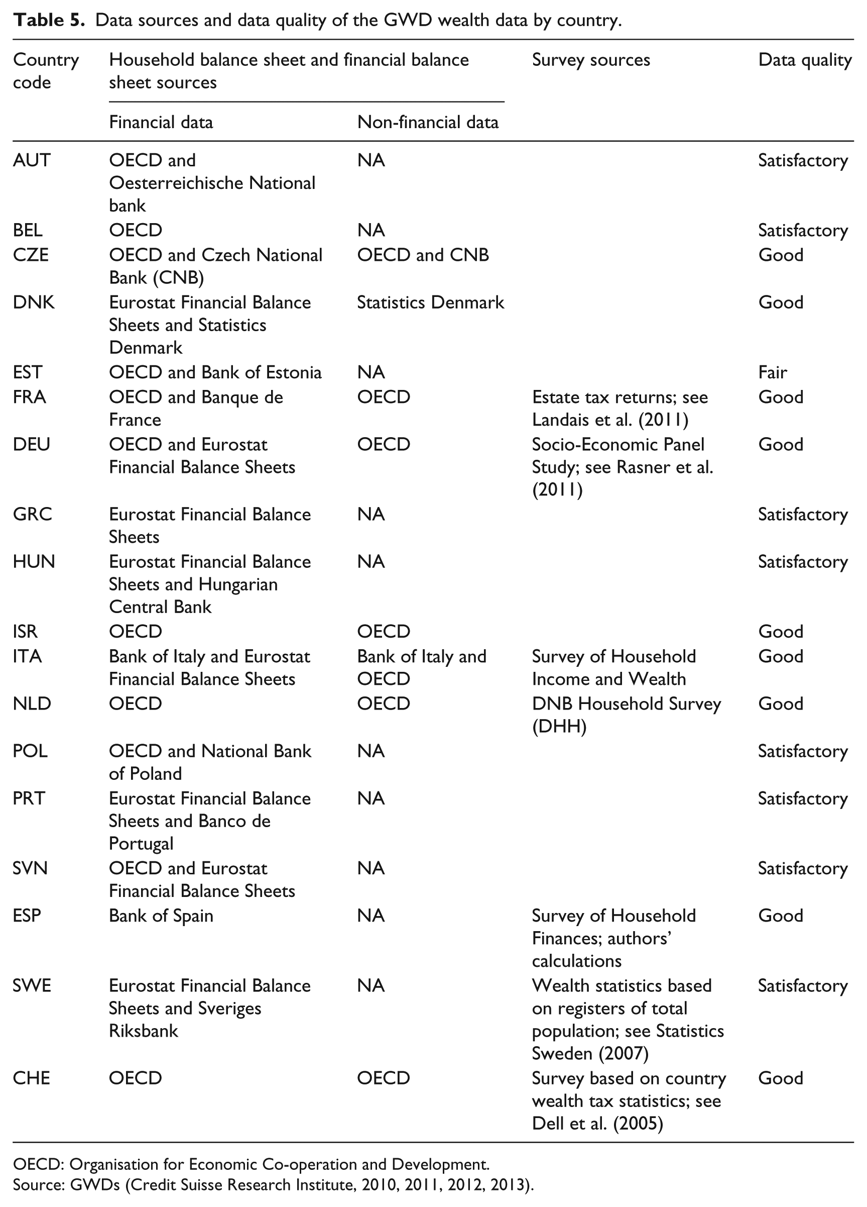
The third step addresses the fact that the traditional sources of wealth distribution data are unlikely to provide an accurate picture of wealth ownership in the top-tail of the distribution. Therefore, the authors make use of the information in the ‘Rich Lists’ published, for example, by Forbes Magazine. With the help of this data, they can adjust the wealth distribution pattern in the highest wealth ranges. Table 5 in the Appendix 1 provides an overview of the different data sources that the authors applied to derive their final wealth measures as published in the GWDs. In addition, the last column provides information about the data quality of each country’s wealth measures as calculated by Shorrocks and Davies. They built a five-point scale to account for data quality. A five-point (‘good’) rating means that the country has complete HBS data, and either wealth distribution data or a good basis for estimating the shape of the wealth distribution. A four point (‘satisfactory’) rating means that the country fulfills all requirements of a ‘good’ rating except that their HBS data does not cover non-financial assets. If a country has no HBS data but a household wealth survey or other wealth distribution data (from estate tax or wealth tax sources), it receives a three point (‘fair’) rating. All 18 countries of our dataset range between three and five points of data quality.

Data on levels of income and income inequality we derived from the OECD iLibrary (OECD, 2013). We merged the OECD income and the GWD wealth information for the overall (20+) population in the 18 above-mentioned countries and derived a second data sample. To balance likewise for yearly variations in household income and wealth, we made use of all four GWD publications (2010–2013), and we chose a similar period for our OECD income measure (explained below). We will conduct all analyses separately with both data samples and compare results.

As mentioned above, there exist at least two additional internationally comparative wealth surveys, the LWS and the HFCS. The LWS covers 12 countries over very different periods. For two countries (Finland and the Unites States), the data go back as far as 1994, while for the rest of the countries, the earliest wealth measures originate from either 1999 or 2000. For the Unites States, six waves are currently available (2000–2006). For all other countries, however, the LWS covers only two (Finland: 1994, 1998; Germany: 2001, 2006; Italy: 2002, 2004) or even only one point in time (Austria: 2004; Canada: 1999; Cyprus: 2002; Japan: 2003; Luxembourg: 2007; Norway: 2002; Sweden: 2002; United Kingdom: 2000) (cf. LWS Variable List, n.d.). Due to the heterogeneity of time points within these datasets, and because the countries only partly overlap with the SHARE countries, we decided to refrain from additionally using the LWS data. The second cross-national wealth survey, which started only very recently, is the HFCS. The first wave data was only released in April 2013. The HFCS covers 18 countries: Austria, Belgium, Cyprus, Estonia, Finland, France, Germany, Greece, Ireland, Italy, Latvia, Luxembourg, Malta, the Netherlands, Portugal, Slovakia, Slovenia, and Spain. The HFCS would doubtless have been a worthwhile supplement to our SHARE and GWD/OECD data. However, because the HFCS covers only one point in time to date, and measures income in terms of gross income – whereas the SHARE and OECD data provide net income – we decided again to refrain from using it in this study, in order to keep problems of comparability to a minimum.

Variables and methods

Our two variables of main interest are household wealth and household income. Household wealth is measured in both surveys in terms of household net worth, which means real assets, plus financial assets, net of debts on them, and refers to current net worth at the time the interview was conducted. The second SHARE wave was conducted between 2006 and 2007 with the exception of Israel, where the second wave was conducted between 2009 and 2010. The fourth SHARE wave was conducted between 2010 and 2012. The GWD wealth variables refer to the years 2010–2013.

In the SHARE data, net worth is defined as follows: (1) gross real assets, that is, the ownership and value of the primary residence, of other real estate, of the share owned of own businesses and of owned cars; plus (2) gross financial assets, that is, the ownership and value of bank accounts, government and corporate bonds, stocks, mutual funds, individual retirement accounts, and contractual savings for housing and life insurance policies; minus (3) mortgages and financial liabilities (Christelis et al., 2005: 358). The target population of individuals in the first SHARE wave is ‘all individuals born in 1954 or earlier, speaking the official language of the country and not living abroad or in an institution such as a prison during the duration of the field work’ (Munich Center for the Economics of Ageing, 2013). In addition, spouses or partners living in the same household are interviewed independent of their age.

A typical problem with questions addressing financial aspects is a high rate of item nonresponse (Riphahn and Serfling, 2005). This applies particularly to persons at the edges of the distribution (i.e. low and high earners). Losing cases due to missing values does increase the risk of ending up with a biased and probably highly selective sample (Kalwij and van Soest, 2005). Therefore, surveys usually apply specific techniques to impute these missing values. The SHARE data has been criticized for showing high numbers of missing values. Item nonresponse in the SHARE is relatively high for both the asset questions on the amount in checking and savings accounts and for the amount in stocks and shares. Percentages of missing values for these variables range from 4.5 percent in Sweden to 13.6 percent in France (Kalwij and van Soest, 2005: 131). However, Kalwij and van Soest (2005) were able to show that, compared to the very well-established English Longitudinal Study of Ageing (ELSA) and the Health and Retirement Study (HRS), the number of missing values for financial questions in SHARE is not significantly higher, and that in some regards the SHARE even outperforms the HRS.

The SHARE team applies a multiple imputation strategy for filling in missing values for both household wealth and household income. Five values are estimated for every missing value. The values are imputed based on observed values of other respondents who are similar, in certain relevant aspects, to the respondent in question. Before applying the imputation procedure, however, the SHARE team applies the so-called ‘unfolding brackets’ procedure. Respondents answering questions on financial values with ‘Don’t know’ or ‘I’d rather not say’ are asked a number of subsequent questions on whether the amount is larger than, smaller than, or about equal to a given amount. Kalwij and van Soest (2005) report that a large fraction of initial item non-respondents answered the bracket questions.⁶

The SHARE team assumes that missing values are missing at random ‘conditional on the set of variables used to determine which respondents are similar to the respondent with the missing value’ (Kalwij and van Soest, 2005: 128f; Little and Rubin, 1987). More precisely, they apply a two-stage imputation procedure. In the first stage, they impute a set of ten core variables (employment income, self-employment income, public pension income per month, private occupational pension income per month, food expenditures per month, value of savings and checking accounts, value of stocks and shares, value of the house (for homeowners), housing rent (for renters) and out-of-pocket outpatient health care expenditures over the last 12 months). In the second stage, all other variables that suffer from item nonresponse are imputed, using the imputed core set variables as conditioning variables.

Kalwij and van Soest (2005) also give an illustration of whether or not the imputations change the conclusions of an issue of interest to SHARE researchers by presenting an analysis of the association between the health status (self-reported health and grip strength) of the respondent and household wealth and income. In their analyses, they use two samples: the first sample includes all observations and the second sample includes only the observations for which no imputations have been made in any of the explanatory variables. In line with previous research, they find a positive relationship between income and health as well as between wealth and health in both samples. However, the magnitudes and significance levels differ. Effects of income and wealth are smaller in the model with imputed values. Based on these findings, we decided to work with the imputed values, which we understand as a more conservative approach.

We run all the following analyses across the five imputations as provided by the SHARE team. All financial values are expressed in Euros and are adjusted for differences in the purchasing power of money across countries and over time using the purchasing power parity (PPP) values as provided by the SHARE team (see Munich Center for the Economics of Ageing, 2013). The reference category is Germany in the year 2005. Furthermore, we divided net worth values by the root of the number of persons living in a household (equivalized household net worth) to account for household size and to increase comparability of the net worth measures from SHARE (household net worth) and GWD (individual net worth). Our final net worth measure is the mean value of annual median household net worth in the second and fourth SHARE wave. Due to the strong skewness of the wealth distribution, we opted for median instead of mean wealth. In order to prevent problems of comparability of values of net worth across countries and between the two datasets to the greatest possible extent and to be consistent with previous research, we derived an additional wealth measure by dividing median net worth by median disposable income, and express net worth in times of disposable income. We label this measure ‘wealth rate’.

The net worth measure in the GWDs is defined as the marketable value of financial assets plus non-financial assets (principally housing and land) less debts for individuals aged 20 or above. All net worth values are expressed in Euros to make them most comparable to the SHARE data.⁷ For reasons already explained above, we decided on median net worth as the final wealth variable and, again, we calculated the wealth rate. Importantly, the current value of public and occupational pension plans is not included, neither in the SHARE nor in the GWD net worth measure.

Household income in the SHARE waves two and four refers to yearly household net income in the year before the interview took place. Household total net income is equal to the sum of the individual-level values of all household members’ annual net income from employment and self-employment; annual public old-age pensions, and other forms of public pensions; annual public long-term insurance payments; annual sum of private long-term care insurance payments; and annual life insurance payment received. To this, the sum of the following household-level variables is added: annual other household members’ net income, interest income from bank accounts, interest income from bonds, dividends from stocks and shares, and interest and dividend income from mutual funds (Munich Center for the Economics of Ageing, 2013: 31). Our final SHARE income measure is the mean of median PPP-adjusted annual net household income from waves two and four. All values are expressed in Euros, and divided by the root of the number of persons living in each household (equivalized household income) to account for household size.

The OECD defines disposable income as ‘Household net adjusted disposable income’, that is, the average amount of money that a household earns per year, after taxes. Again, we express all income values in Euros. To likewise balance yearly variation in income, our income measure is calculated as the mean of median disposable household income of the years 2007–2010, in order to come closest to the period the GWD wealth measure is based upon.

In our descriptive analyses, for the SHARE data, we apply weights in accordance with the recommendations of the SHARE team. We use cross-sectional calibrated weights that compensate for unit nonresponse and sample attrition in the CAPI interviews (Munich Center for the Economics of Ageing, 2013: 40). The level of inequality in income and wealth we measure via the Gini coefficient, which is provided for the GWD and OECD data and which we calculated for the SHARE data according to the following formula

G (w) = [\frac{1}{2 n^{2} μ}] \sum_{i = 1}^{n} n \sum_{j = 1} | w_{i} - w_{j} |

(1)

with inequality G in wealth w (or likewise in income y) measured by the arithmetic average of the absolute difference between all wealth (or income) pairs standardized by dividing it by the population’s average wealth (or income). As a result the Gini index ranges from 0 (total equality) to 1 (total inequality). Apart from being the best known measure of inequality in social sciences, Gini has another considerable advantage for our purpose: it is well defined for negative and zero values (Jenkins and Jäntti, 2005: 20),⁸ which are likely to appear in the distribution of private net worth. We express all Gini values as multiplied by 100.

In order to categorize countries by their resemblance in terms of income inequality and wealth inequality, we use a standard hierarchical cluster analysis method, the Ward’s linkage cluster analysis. Hierarchical cluster analysis algorithms are either agglomerative or divisive: The latter begin by including all of the observations in one cluster and subsequently proceed to split them into smaller clusters; the former, on the other hand, start with each observation being treated as a separate cluster and proceed to combine those until the threshold level in a dissimilarity measure is reached. The Ward’s linkage cluster analysis is an agglomerative method that minimizes the error sum of squares of any two (hypothetical) clusters that can be formed at each step of clustering.⁹ At each stage, the method aims to minimize the increase in the total within-cluster error sum of squares. The Ward cluster analysis is regarded as very efficient but tends to create clusters of small though equal size (Everitt, 2011: 77ff).

Analyses and results

The distribution of private wealth

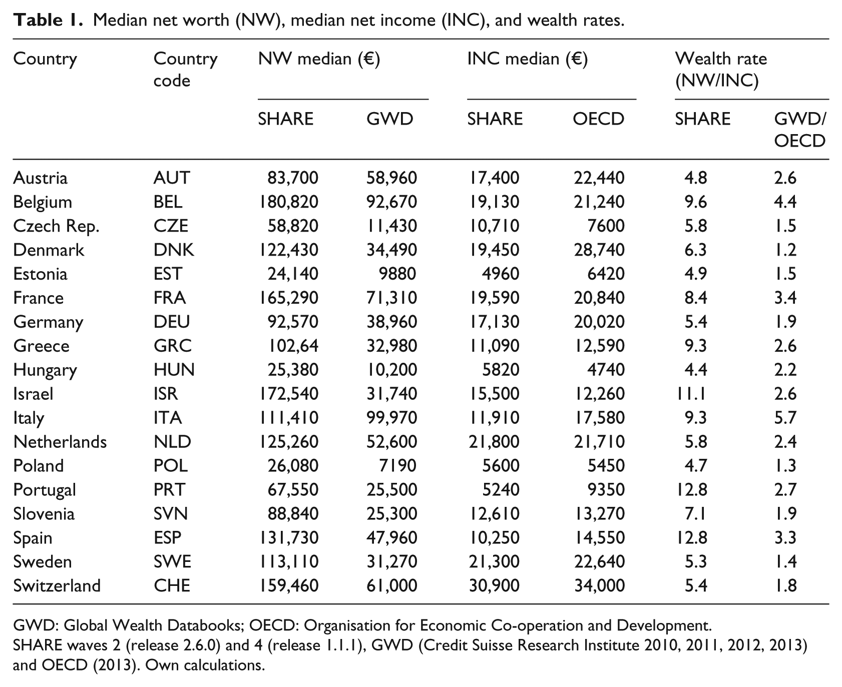
Table 1 shows the distribution of net worth and disposable income as well as the wealth rate (median net worth divided by median income) across the 18 countries in our SHARE and GWD/OECD datasets. Looking at median values of net worth, we can first see that – with only very few exceptions – net worth values are higher among the 50+ SHARE than among the 20+ GWD population, which corresponds to the assumptions of the life-cycle hypothesis. In the SHARE data, the highest values for median net worth can be found in Belgium (€180,820), Israel (€172,540), and France (€165,290), followed by Switzerland (€159,460). The lowest values can be found in Estonia (€24,140) and Hungary (€25,380). In the GWD data, the highest values for median net worth can be found in Italy (€99,970), Belgium (€92,670) and France (€71,310). The lowest values emerge in Poland (€7190), Hungary (€10,200) and the Czech Republic (€11,430). Trends in median net worth show a similar tendency in the two datasets, which can be understood as an indicator of good data quality.

Table 1.

Median net worth (NW), median net income (INC), and wealth rates.

Country	Country code	NW median (€)		INC median (€)		Wealth rate (NW/INC)
Country	Country code	SHARE	GWD	SHARE	OECD	SHARE	GWD/OECD
Austria	AUT	83,700	58,960	17,400	22,440	4.8	2.6
Belgium	BEL	180,820	92,670	19,130	21,240	9.6	4.4
Czech Rep.	CZE	58,820	11,430	10,710	7600	5.8	1.5
Denmark	DNK	122,430	34,490	19,450	28,740	6.3	1.2
Estonia	EST	24,140	9880	4960	6420	4.9	1.5
France	FRA	165,290	71,310	19,590	20,840	8.4	3.4
Germany	DEU	92,570	38,960	17,130	20,020	5.4	1.9
Greece	GRC	102,64	32,980	11,090	12,590	9.3	2.6
Hungary	HUN	25,380	10,200	5820	4740	4.4	2.2
Israel	ISR	172,540	31,740	15,500	12,260	11.1	2.6
Italy	ITA	111,410	99,970	11,910	17,580	9.3	5.7
Netherlands	NLD	125,260	52,600	21,800	21,710	5.8	2.4
Poland	POL	26,080	7190	5600	5450	4.7	1.3
Portugal	PRT	67,550	25,500	5240	9350	12.8	2.7
Slovenia	SVN	88,840	25,300	12,610	13,270	7.1	1.9
Spain	ESP	131,730	47,960	10,250	14,550	12.8	3.3
Sweden	SWE	113,110	31,270	21,300	22,640	5.3	1.4
Switzerland	CHE	159,460	61,000	30,900	34,000	5.4	1.8

GWD: Global Wealth Databooks; OECD: Organisation for Economic Co-operation and Development.

SHARE waves 2 (release 2.6.0) and 4 (release 1.1.1), GWD (Credit Suisse Research Institute 2010, 2011, 2012, 2013) and OECD (2013). Own calculations.

With regard to disposable income, readers have to be aware of the fact that, in the SHARE data, a meaningful fraction of each country’s population is already retired and receives transfer incomes only (mainly pension income). The highest values for median net income in the SHARE data emerge in Switzerland (€30,908), Sweden (€21,294), and the Netherlands (€21,804) and in the OECD data again in Switzerland (€34,000) and Denmark (€28,740). The lowest values for median net income due to both datasets emerge in the Eastern European countries Estonia, Hungary, Slovenia and the Czech Republic, closely followed by the Southern European countries Portugal, Greece, Spain, and Italy.

The next two columns show the wealth rate (median net worth divided by median income), relating a country’s level of net worth directly to its level of net income. In the SHARE data, the highest wealth rates (wr) appear in Portugal and Spain, where older households hold values of median net worth more than 13 times greater than their (last year’s) disposable income. Portugal and Spain are followed by Israel (wr = 11.1), Belgium (wr = 9.6), Greece and Italy (wr = 9.3). Also, in the GWD data, the two Southern European countries Italy (wr = 5.7) and Spain (wr = 3.3) show comparatively high wealth rates. High wealth rates emerge also in Belgium (wr = 4.4) and France (wr = 3.4). In general, wealth rates are much higher in the SHARE than in the GWD data, which should principally be a result of the different population groups in terms of age. The lowest wealth rates in the SHARE data emerge in Hungary (wr = 4.4), Austria (wr = 4.8) and Estonia (wr = 4.9), and in the GWD data in Denmark (wr = 1.2), Poland (wr = 1.3), and Sweden (wr = 1.4).

Altogether, high levels of median wealth (in times of median income) emerge in the Southern European countries (SHARE: Greece, Portugal, Spain; GWD/OECD: Italy, Portugal, Spain), where median income is comparatively low, but also in Belgium (SHARE and GWD/OECD) and Israel (SHARE). Low levels of median wealth (in times of median income) emerge in the Eastern European countries (SHARE: Estonia, Hungary, Poland; GWD/OECD: Estonia, Poland), where median income is low as well, but also in Austria (SHARE) and in the Northern European countries Denmark and Sweden (GWD/OECD), where median income is high.

National patterns of wealth and income inequality

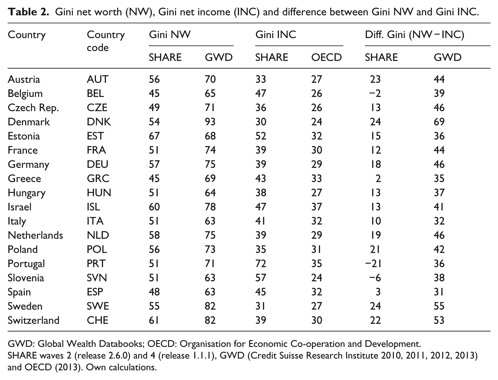
Table 2 shows our findings for the levels of income and wealth inequality in the SHARE and the GWD/OECD datasets. In the SHARE data, the highest values for inequality in net worth emerge in Estonia (Gini = 67), Switzerland (Gini = 61) and Israel (Gini = 60), in the GWD data in Denmark (Gini = 93), Sweden (Gini = 82), and Switzerland (Gini = 82). The lowest values for wealth inequality according to the SHARE data emerge in Belgium and Greece (Gini = 45), Spain (Gini = 48), and the Czech Republic (Gini = 49), and according to the GWD data in Italy, Slovenia, and Spain (Gini = 63), followed by Hungary (Gini = 64) and Belgium (Gini = 65). The trends in the levels of wealth inequality reported by the SHARE data resemble those found in the GWD data for most countries. Exceptions are Estonia, which shows a below-median level of wealth inequality in the GWD data, but a level of wealth inequality considerably above the median in the SHARE data. Similar strong differences between the two datasets emerge for Slovenia.

Table 2.

Gini net worth (NW), Gini net income (INC) and difference between Gini NW and Gini INC.

Country	Country code	Gini NW		Gini INC		Diff. Gini (NW − INC)
Country	Country code	SHARE	GWD	SHARE	OECD	SHARE	GWD
Austria	AUT	56	70	33	27	23	44
Belgium	BEL	45	65	47	26	−2	39
Czech Rep.	CZE	49	71	36	26	13	46
Denmark	DNK	54	93	30	24	24	69
Estonia	EST	67	68	52	32	15	36
France	FRA	51	74	39	30	12	44
Germany	DEU	57	75	39	29	18	46
Greece	GRC	45	69	43	33	2	35
Hungary	HUN	51	64	38	27	13	37
Israel	ISL	60	78	47	37	13	41
Italy	ITA	51	63	41	32	10	32
Netherlands	NLD	58	75	39	29	19	46
Poland	POL	56	73	35	31	21	42
Portugal	PRT	51	71	72	35	−21	36
Slovenia	SVN	51	63	57	24	−6	38
Spain	ESP	48	63	45	32	3	31
Sweden	SWE	55	82	31	27	24	55
Switzerland	CHE	61	82	39	30	22	53

GWD: Global Wealth Databooks; OECD: Organisation for Economic Co-operation and Development.

SHARE waves 2 (release 2.6.0) and 4 (release 1.1.1), GWD (Credit Suisse Research Institute 2010, 2011, 2012, 2013) and OECD (2013). Own calculations.

The highest income inequalities according to the SHARE data can be found in Portugal (Gini = 72) and Slovenia (Gini = 57), and according to the OECD data in Portugal (Gini = 35) and Israel (Gini = 37). The lowest values for income inequality emerge in Denmark (Gini = 30), Sweden (Gini = 31) and Austria (Gini = 33) according to the SHARE data, and in Denmark and Slovenia (Gini = 24), followed by Belgium and the Czech Republic (Gini = 26) and then Austria, Hungary, and Sweden (Gini = 27) according to the OECD data. As to the national patterns of income inequality, the results of the SHARE resemble those of the OECD data and those of past research. In general, income inequalities are higher among the 50+ population than among the 20+ population. We were able to find meaningful differences between the two datasets for Slovenia and Belgium. While the SHARE data reports above-median levels of income inequality in those countries, in the OECD data they are below-median level.

Altogether, the lowest levels of wealth inequality we find in the Southern European countries which showed the highest wealth rates (SHARE, GWD: Greece, Italy, Spain), but also in Belgium and Slovenia (SHARE, GWD). Surprisingly, we find the highest levels of wealth inequality in the Northern European countries Sweden (SHARE, GWD) and Denmark (GWD), which show the lowest levels of income inequality but also in Switzerland (SHARE, GWD). Central and Eastern European countries are distributed over the full range of levels of wealth inequality.

The last two columns show the differences between the Gini values for income and wealth inequality for each country. This informs us whether a country’s levels of income and wealth inequality are either similar to or different from each other. We can see first that, in all countries except Belgium, Portugal, and Slovenia (but only in the SHARE data), levels of wealth inequality are higher than levels of income inequality, which is in line with theory as well as with past empirical findings (e.g. Davies et al., 2008). Similar levels of income and wealth inequality in the SHARE data can be found in Belgium, Greece, Slovenia, and Spain. Large discrepancies emerge in Denmark, Sweden, Austria, and Switzerland. According to the GWD/OECD data, income and wealth inequalities are similar in Spain, Italy and Greece, and more dissimilar in Denmark, Sweden, and Switzerland. As before, trends emerging from the SHARE data, on the one hand, and from the GWD/OECD data, on the other hand, are similar to each other, indicating good data quality, but may also point to the relative stability of patterns of wealth inequality over the life course.

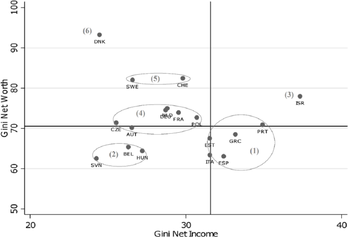
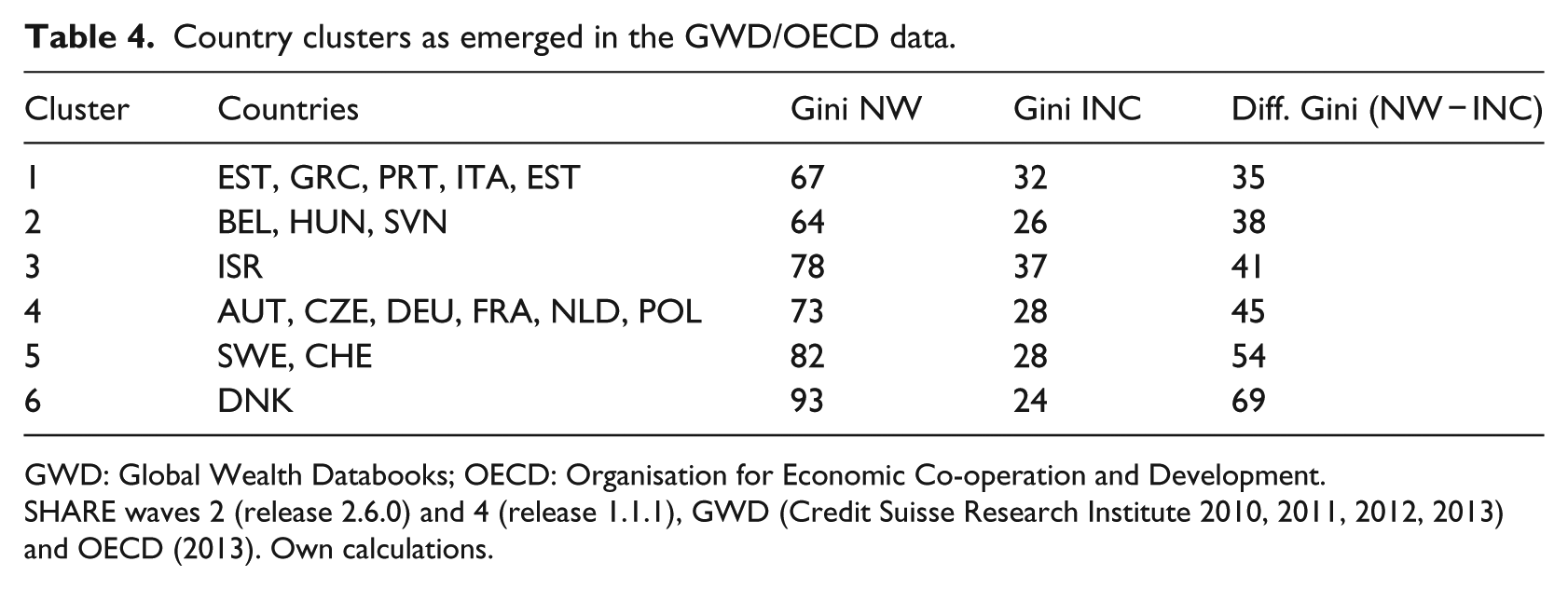
Figure 1 (SHARE data) and Figure 2 (GWD/OECD data) illustrate the findings of Table 2 in simple scatterplots and show the results of our cluster analyses. For both datasets, we applied a Ward’s linkage cluster analysis. In the SHARE data, we opted for a 4-cluster solution, while in the GWD data, we prioritized the 6-cluster solution.¹⁰ The thick lines represent median levels of income and wealth inequality (Gini) over all countries in each dataset. We can see, first, that there is a larger variance of levels of income inequality in the SHARE (older population) than in the OECD (overall population) dataset, while variance in levels of wealth inequality is larger in the GWD (overall population) than in the SHARE (older population) data. The median level of income inequality is higher in the SHARE (Gini = 39) than in the OECD (Gini = 29) data, and the median level of wealth inequality is higher in the GWD (Gini = 71) than in the SHARE (Gini = 54) data. Second, the heterogeneity and variance with regard to national levels of income and wealth inequality is larger in the GWD than in the SHARE data.

Figure 1.

Gini of income and wealth inequality: SHARE data.

Figure 2.

Gini of income and wealth inequality: GWD/OECD data.

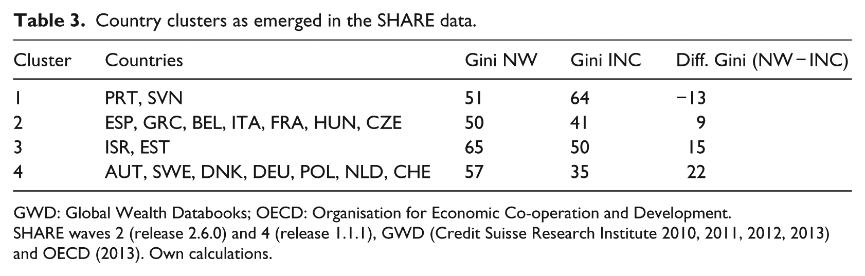
In the SHARE data we find two larger clusters (each made up of seven countries) and two smaller clusters (each made up of two countries). In Table 3, for each cluster of the SHARE data, the Gini coefficients for income and wealth as well as the difference between levels of wealth and income are displayed. We sorted clusters in ascending order according to the numerical difference between levels of wealth and income inequality. The first cluster is a special cluster, characterized by a level of wealth inequality which is below the level of income inequality. This cluster consist of Portugal and Slovenia. The countries in the second cluster can be characterized by medium levels of income inequality and below average levels of wealth inequalities. It consists of three Southern European countries (Spain, Greece, and Italy), but also two Central European countries (Belgium and France) and two Eastern European countries (Hungary and the Czech Republic). The third cluster is made up of two countries (Israel and Estonia) that show very high levels of income inequality combined with very high levels of wealth inequality. Finally, the fourth cluster consists of the two Northern European countries in the SHARE data (Denmark and Sweden), as well as of four Central European countries (Austria, Germany, the Netherlands, and Switzerland) and one Eastern European country (Poland). These countries can be characterized by levels of income and wealth inequality close to the average levels of these two measures.

Table 3.

Country clusters as emerged in the SHARE data.

Cluster	Countries	Gini NW	Gini INC	Diff. Gini (NW − INC)
1	PRT, SVN	51	64	−13
2	ESP, GRC, BEL, ITA, FRA, HUN, CZE	50	41	9
3	ISR, EST	65	50	15
4	AUT, SWE, DNK, DEU, POL, NLD, CHE	57	35	22

GWD: Global Wealth Databooks; OECD: Organisation for Economic Co-operation and Development.

SHARE waves 2 (release 2.6.0) and 4 (release 1.1.1), GWD (Credit Suisse Research Institute 2010, 2011, 2012, 2013) and OECD (2013). Own calculations.

With the GWD/OECD data, we opt for a 6-cluster solution. Table 4 gives an overview of the levels of income and wealth inequality of each of these clusters as well as the absolute distance between the two measures. Again, we sorted clusters in ascending order according to the numerical difference between levels of wealth and income inequality. In the GWD/OECD data, we do find no countries with levels of wealth inequality below levels of income inequality. The first cluster is made up of countries with above average levels of income inequality but below or close to average levels of wealth inequality. This cluster consists of all four Southern European countries in the data (Greece, Italy, Portugal, and Spain) and one Eastern European country (Estonia). The countries of the second cluster show, likewise, below or close to average levels of wealth inequality combined with below average levels of income inequality. These are two Eastern European countries (Hungary, Slovenia) and one Central European country (Belgium). Israel makes up the third cluster, showing above average levels of wealth and income inequality. The fourth cluster is fairly similar to the fourth SHARE cluster. It combines countries with close to average levels of wealth and income inequality. Four Central European countries (Austria, Germany, the Netherlands, and France) and two Eastern European countries (the Czech Republic and Poland) make up this cluster. The fifth cluster consists of two countries, one Central European country (Switzerland), and one Northern European country (Sweden), which exhibit below or very close to average levels of income inequality combined with above average levels of wealth inequality. There remains another Northern European country, Denmark, which shows an extraordinarily high level of wealth inequality combined with a below average level of income inequality.

Table 4.

Country clusters as emerged in the GWD/OECD data.

Cluster	Countries	Gini NW	Gini INC	Diff. Gini (NW − INC)
1	EST, GRC, PRT, ITA, EST	67	32	35
2	BEL, HUN, SVN	64	26	38
3	ISR	78	37	41
4	AUT, CZE, DEU, FRA, NLD, POL	73	28	45
5	SWE, CHE	82	28	54
6	DNK	93	24	69

GWD: Global Wealth Databooks; OECD: Organisation for Economic Co-operation and Development.

SHARE waves 2 (release 2.6.0) and 4 (release 1.1.1), GWD (Credit Suisse Research Institute 2010, 2011, 2012, 2013) and OECD (2013). Own calculations.

Discussion and conclusion

Despite its importance in the process of social stratification, previous research has paid too little attention to wealth, being preoccupied with the determination of individual attainment (Kenworthy, 2007). In the light of demographic and social changes, measures solely related to the individual’s position in the labor market are increasingly less suited to capturing a society’s level of social inequality. Only recently has there been a growing awareness among researchers that wealth is not merely an additional, but also a separate dimension of social stratification and of social inequality. With this article, we contribute to this growing awareness by drawing attention to wealth.

More precisely, we addressed two research questions here. First, we wanted to find out how private wealth is distributed internationally, and second, we were interested to see if national patterns of wealth inequality resemble national patterns of income inequality. We applied the Ward’s linkage cluster analysis to find clusters of countries, which are similar to one another regarding the levels of wealth and income inequality they exhibit.

Theoretically, there are reasons to assume both similarity and dissimilarity in a country’s levels of income and wealth inequality. It is important to mention that wealth can stem from two sources, transfers and self-accumulation (income minus consumption). Wealth can be accumulated by saving (investing) parts of one’s income. Saving depends first on the ability to save and second on preferences to save. Finally, saving also depends on the perceived necessity to save. If most of the wealth in a country is life-cycle wealth, then it is fair to assume that earnings differences strongly translate into wealth differences, controlling for individual preferences for saving. Past research, however, showed that there are meaningful differences in levels of income and wealth inequality for a number of countries (e.g. for Sweden: Roine and Waldenström, 2009).

In our study, we analyzed and compared the distributions of income and wealth from two different data sets referring to two different population segments (SHARE: 50+ population, GWD/OECD: 20+ population) in 17 European countries and Israel. Our results showed the following: first, we found meaningful differences in levels of household wealth between countries, and second, we found levels of wealth inequality to also differ strongly across countries. This clustering only partly corresponds to the national grouping based on levels of income inequality. We found as many countries with similar levels of income and wealth inequality as countries with strong differences in their levels of income and wealth inequality.

We applied hierarchical clustering methods to find clusters of countries that are similar to each other with regard to their levels of income and wealth inequality. In the SHARE data we selected a 4-cluster solution, while in the GWD/OECD data we opted for a 6-cluster solution. Although we found the clusters of the two datasets to significantly differ from one another, we also found some very interesting similarities. First, in both datasets the Southern European countries are to be found in clusters that exhibit close to or above average levels of income inequality combined with below average levels of wealth inequality. The Northern European countries, on the other hand, combine close to or below average levels of income inequality with above average levels of wealth inequality in both datasets. In addition, Switzerland shows an average level of income inequality with above average levels of wealth inequality in both datasets. Outlying in both datasets is Israel, with above average levels in both income and wealth inequality. The Central and Eastern European countries, however, we found to be distributed over different clusters.

Most surprising is certainly the finding that the Northern European countries – known for their high level of social equality – exhibit high levels of wealth inequality, although a number of studies have already reported this phenomenon, most of them for Sweden (Domeij and Klein, 2002; Piketty, 2014: 344f; Roine and Waldenström, 2009; Sierminska et al., 2006), and also several for Denmark (Bjørnskov et al., 2012; Davies et al., 2009). Domeij and Klein (2002: 505) suggest that the generous public pension system in Sweden (with a common benefit payable to each senior, as well as an upper limit to earnings-related pension benefits) can explain the differences in the levels of income and wealth inequality to a large degree, as it reduces incentives for the low income-earners to save proportionately more compared to the high-income earners. Roine and Waldenström (2009) add that the wealth concentration in Sweden increased dramatically after 1980, due to ‘dramatic increases in stock returns at the Stockholm Stock Exchange between 1980 and 2000’ (p. 170). In the same period, the value of large privately held family firms, making up an important share of Swedish private net worth, grew rapidly (Roine and Waldenström, 2009: 169). For Denmark, Davies et al. (2009) report a Gini coefficient for wealth inequality in 1996 of 0.81.¹¹ This is similar to our mean Gini of 0.93 as reported in the GWD data for the years 2010–13. Possible explanations for the extraordinarily high level of wealth inequality in Denmark are the easy access to mortgage or loans accompanied by a high level of debts in the Danish population, as well as the low number of homeowners. Andersen et al. (2012) report a very high debt-to-income ratio in Danish households when compared to other nations. However, they acknowledge that the largest share of debts is held by high-income families, indicating that the debt is often raised in order to finance purchases of luxury goods (e.g. a larger home) (Andersen et al., 2012: 1). Nevertheless, there is still a reasonable percentage of household with positive net debt of more than 30 percent (Andersen et al., 2012: 1), which is likely to drive the high level of wealth inequality in Denmark.

An aspect not considered in this article is the composition of wealth. National differences in the household wealth portfolio are, however, an important determinant of national differences in the distribution of wealth, as shown by past research (Keister and Moeller, 2000; Skopek et al., 2012; Spilerman, 2000) and share different advantages and disadvantages. Compared to financial assets such as shares, bonds, or money in bank accounts, housing wealth is, for example, much less mobile and less easy to liquidize. On the other hand, compared to real assets, financial assets are much more subject to interest rate changes and inflation.

Among the different types of wealth, owner-occupied housing is of particular importance as it is the quantitatively most important component of household wealth in most countries in our analysis (cf. Kolb et al., 2013). Moreover, housing wealth was found to have an equalizing effect on wealth inequality in these countries (Skopek et al., 2012). Households in the Mediterranean countries, for example, hold most of their wealth in the form of residential property, which is of much less importance in Germany, where households’ wealth portfolios are more diversified. In Denmark, the share of homeowners is extraordinarily low. In 2010, only 43 percent of all households were homeowners, meaning that 57 percent were tenants (Bjørnskov et al., 2012). Various studies have found that the Danish homeownership rates have stagnated or even decreased over the last decade (Pohl Nielsen and Blume Jensen, 2011; Skak, 2006), which stands in contrast to other European and North-American countries. There seems to be a positive correlation between high rates of homeownership, on the one hand, and high median values of net worth together with comparatively low levels of wealth inequality, on the other hand. At the same time, the high rate of homeownership, correlating with a high level of net worth, in the Mediterranean countries might be a result of the poor performance of the public pension system. A recent study of Frick and Grabka (2013) supports this argument. The authors criticize the fact that the ‘standard’ concept of net worth as applied in most surveys ignores any entitlements to public pension schemes. In their study, based on German panel data, Frick and Grabka (2013) calculate an extended measure of wealth by combining public pension and private wealth. Doing this, median net worth increases by 70 percent, with public pension entitlements making up about 40 percent of total net worth. In addition, the level of wealth inequality (Gini coefficient) is reduced by one quarter, suggesting an impact of public pension wealth not only on a country’s level of wealth, but also on its level of wealth inequality.

Moreover, we did not pay special attention to the importance of inheritances or transfers. While it is not clear, which is the contribution of inherited or transferred wealth to total wealth, one can assume that if most wealth is transferred wealth, the distribution of wealth might be much more dependent on the taxation of wealth or inheritances. This becomes even more important in the light of the expected ‘inheritance wave’. The last 70 years have been a period of peace and economic prosperity in most industrialized countries of the Western world. During this time, households have been able to accumulate substantial amounts of wealth. The cohort living and working during this period is now in its 50s–70s and is expected to bequeath a historically unprecedented amount of wealth to their children (the baby boomer generation, born between 1946 and 1964) and grandchildren. For Germany, researchers expect a trillion Euros more to be inherited between 2010 and 2020 as compared to the decade before, which represents an increase of 50 percent (Die Welt, 2011). Similar amounts of wealth are expected, for example, for the baby boomers in Canada (Yew, 2012). However, researchers are divided over the impact of inheritances on the distribution of wealth (Karagiannaki, 2011; Kohli et al., 2006; Szydlik, 2004).

So what do these findings imply? First and foremost, our results strongly suggest that income and wealth should be treated as two distinct dimensions of social stratification. In light of the growing importance of wealth as an income substitute in older age and during retirement, stratification research should focus on wealth inequalities in order to gain a comprehensive understanding of the level of social inequality in modern societies. Moreover, the results of our article can be understood as an indicator that the current definition of poverty – which is based solely on income in Europe and on income combined with consumption in the Unites States – is too shortsighted. Considering wealth in addition to income can significantly change the economic position of a household or individual. Summing up, we propose that our article lays an important foundation for research on the sources and consequences of wealth and wealth inequality. Especially interesting, in this respect, are the groups of nations with different levels of income and wealth inequality: broadly, the Northern and Southern European countries.

Footnotes

Appendix 1

Table 5.

Data sources and data quality of the GWD wealth data by country.

Country code	Household balance sheet and financial balance sheet sources		Survey sources	Data quality
	Financial data	Non-financial data
AUT	OECD and Oesterreichische National bank	NA		Satisfactory
BEL	OECD	NA		Satisfactory
CZE	OECD and Czech National Bank (CNB)	OECD and CNB		Good
DNK	Eurostat Financial Balance Sheets and Statistics Denmark	Statistics Denmark		Good
EST	OECD and Bank of Estonia	NA		Fair
FRA	OECD and Banque de France	OECD	Estate tax returns; see Landais et al. (2011)	Good
DEU	OECD and Eurostat Financial Balance Sheets	OECD	Socio-Economic Panel Study; see Rasner et al. (2011)	Good
GRC	Eurostat Financial Balance Sheets	NA		Satisfactory
HUN	Eurostat Financial Balance Sheets and Hungarian Central Bank	NA		Satisfactory
ISR	OECD	OECD		Good
ITA	Bank of Italy and Eurostat Financial Balance Sheets	Bank of Italy and OECD	Survey of Household Income and Wealth	Good
NLD	OECD	OECD	DNB Household Survey (DHH)	Good
POL	OECD and National Bank of Poland	NA		Satisfactory
PRT	Eurostat Financial Balance Sheets and Banco de Portugal	NA		Satisfactory
SVN	OECD and Eurostat Financial Balance Sheets	NA		Satisfactory
ESP	Bank of Spain	NA	Survey of Household Finances; authors’ calculations	Good
SWE	Eurostat Financial Balance Sheets and Sveriges Riksbank	NA	Wealth statistics based on registers of total population; see Statistics Sweden (2007)	Satisfactory
CHE	OECD	OECD	Survey based on country wealth tax statistics; see Dell et al. (2005)	Good

OECD: Organisation for Economic Co-operation and Development.

Source: GWDs (Credit Suisse Research Institute, 2010, 2011, 2012, 2013).

Acknowledgements

We thank William Tayler (The Bamberg Translation Co.) for his language editing support.

Funding

This work was supported by the German -Israeli Foundation for Scientific Research and Development (Project no.: I - 1021 - 304.4/2008).

Notes

References

Andersen

Christensen

Nielsen

. (2012) The wealth and debt of Danish families. Monetary Review 2: 1–40.

Atkinson

(1971) The distribution of wealth and the individual life-cycle. Oxford Economic Papers 23(2): 239–254.

Attanasio

Hoynes

(2000) Differential mortality and wealth accumulation. The Journal of Human Resources 35(1): 1–29.

Barro

(1978) The Impact of Social Security on Private Saving. Washington, DC: American Enterprise Institute for Public Policy Research.

Bernheim

(1998) Financial illiteracy, education and retirement saving. In: Mitchell

Schieber

(eds) Living with Defined Contributions Pensions. Philadelphia, PA: Pension Research Council, pp. 38–68.

Bjørnskov

Neamtu

Westergård-Nielsen

(2012) Growing inequality and its impact in Denmark. Country report for Denmark. Available at: http://gini-research.org/system/uploads/509/original/Denmark.pdf?1373978704

Bonini

(2007) Cross-national variation in individual life satisfaction: Effects of national wealth, human development, and environmental conditions. Social Indicators Research 87(2): 223–236.

Bourdieu

(1984) Distinction. Oxon: Routledge Kegan & Paul.

Bourdieu

(1986) The forms of capital. In: Richardson

(ed.) Handbook of Theory and Research for the Sociology of Education. New York: Greenwood Press, pp. 241–258.

10.

Cagan

(1965) The Effect of Pension Plans on Aggregate Savings: Evidence from a Sample Survey. New York: National Bureau of Economic Research.

11.

Christelis

Jappelli

Padula

(2005) Wealth and portfolio composition. In: Börsch-Supan

Brugiavini

Jürges

. (eds) Health, Ageing and Retirement in Europe: First Results from the Survey of Health, Ageing and Retirement in Europe. Mannheim: MEA, pp. 310–317.

12.

Conley

(2009) Being Black, Living in the Red: Race, Wealth, and Social Policy in America. Berkeley, CA; Los Angeles, CA: University of California Press.

13.

Cowell

Karagiannaki

McKnight

(2012) Mapping and measuring the distribution of household wealth: A cross-country analysis. CASE working paper 165. Available at: http://sticerd.lse.ac.uk/dps/case/cp/CASEpaper165.pdf

14.

Cowell

Karagiannaki

McKnight

(2013) Accounting for cross-country differences in wealth inequality. CASE working paper 168. Available at: http://sticerd.lse.ac.uk/dps/case/cp/CASEpaper168.pdf

15.

Credit Suisse Research Institute (2010) Global Wealth Databook 2010. Zurich: Credit Suisse Research Institute.

16.

Credit Suisse Research Institute (2011) Global Wealth Databook 2011. Zurich: Credit Suisse Research Institute.

17.

Credit Suisse Research Institute (2012) Global Wealth Databook 2012. Zurich: Credit Suisse Research Institute.

18.

Credit Suisse Research Institute (2013) Global Wealth Databook 2013. Zurich: Credit Suisse Research Institute.

19.

Dahrendorf

(1959) Class and Class Conflict in Industrial Society. Stanford, CA: Stanford University Press.

20.

Davies

Shorrocks

(2000) The distribution of wealth. In: Atkinson

Bourguignon

(eds) Handbook of Income Distribution. Amsterdam; New York: Elvesier, pp. 605–675.

21.

Davies

Sandström

Shorrocks

. (2008) The world distribution of household wealth. United Nations University UNU-WIDER research paper 03. Available at: http://www.wider.unu.edu/publications/working-papers/discussion-papers/2008/en_GB/dp2008-03/

22.

Davies

Shorrocks

Sandström

. (2009) The level and distribution of global household wealth. NBER working paper 15508. Available at: http://www.nber.org/papers/w15508.pdf

23.

Dell

Piketty

Saez

(2005): Income and wealth concentration in Switzerland over the 20th century. CEPR discussion paper 5090. London: Centre for Economic Policy Research. Available at: http://eml.berkeley.edu/~saez/dell-piketty-saezCEPR05suisse.pdf

24.

Die Welt (2011) Auf die Deutschen rollt eine Erbschafts-Welle zu. Available at: http://www.welt.de/finanzen/verbraucher/article13338273/Auf-die-Deutschen-rollt-eine-Erbschafts-Welle-zu.html (accessed 28 August 2014).

25.

DiPrete

Eirich

(2006) Cumulative advantage as a mechanism for inequality: A review of theoretical and empirical developments. Annual Review of Sociology 32(1): 271–297.

26.

Domeij

Klein

(2002) Public pensions: To what extent do they account for Swedish wealth inequality? Review of Economic Dynamics 5(3): 503–534.

27.

Durkheim

(2008) The division of labor in society. In: Grusky

(ed.) Social Stratification: Class, Race and Gender in Sociological Perspective. Boulder, CO: Westview Press, pp. 159–164.

28.

Elder

(1975) Age differentiation and the life course. Annual Review of Sociology 1: 165–190.

29.

Elmelech

(2008) Transmitting Inequality: Wealth and the American Family. Lanham, MD: Rowman & Littlefield Publishers.

30.

Everitt

(2011) Cluster Analysis, 5th edn. Chichester: John Wiley & Sons, Ltd.

31.

Feldstein

(1974) Social security, induced retirement, and aggregate capital accumulation. Journal of Political Economy 82(5): 905–926.

32.

Feldstein

(1995) Fiscal policies, capital formation, and capitalism. European Economic Review 39(3–4): 399–420.

33.

Filmer

Pritchett

(2004) The effect of household wealth on educational attainment: Evidence from 35 countries. Population and Development Review 25(1): 85–120.

34.

Forrester

(1961) Industrial Dynamics. Cambridge, MA: MIT Press.

35.

Forrester

(1968) Principles of Systems. Cambridge, MA: Wright-Allen Press.

36.

Frick

Grabka

(2009a) Wealth inequality on the rise in Germany. DIW Berlin weekly report no. 10/2009, 28 May 2009. Berlin: DIW Berlin, vol. 5, pp. 62–73.

37.

Frick

Grabka

(2009b) Zur Entwicklung der Vermögensungleichheit in Deutschland. Berliner Journal für Soziologie 19(4): 577–600.

38.

Frick

Grabka

(2013) Public pension entitlements and the distribution of wealth. In: Gornick

Jäntti

(eds) Income Inequality: Economic Disparities and the Middle Class in Affluent Countries. Stanford, CA: Stanford University Press, pp. 362–387.

39.

Furnham

(1985) Why do people save? Attitudes to, and habits of, saving money in Britain. Journal of Applied Social Psychology 15(4): 354–373.

40.

Gale

Scholz

(1994) Intergenerational transfers and the accumulation of wealth. The Journal of Economic Perspectives 8(4): 145–160.

41.

Grusky

(ed.) (2008) Social Stratification: Class, Race, and Gender in Sociological Perspective, 3rd edn. Boulder, CO: Westview Press.

42.

Headey

Muffels

Wooden

(2008) Money doesn’t buy happiness: Or does it? A reconsideration based on the combined effects of wealth, income and consumption. Social Indicators Research 87(1): 62–85.

43.

Henretta

Campbell

(1978) Net worth as an aspect of status. The American Journal of Sociology 83(5): 1204–1223.

44.

Hochman

Skopek

(2013) The impact of wealth on subjective well-being: A comparison of three welfare-state regimes. Research in Social Stratification and Mobility 34: 127–141.

45.

Jappelli

(2010) Economic literacy: An international comparison. The Economic Journal 120(548): 429–451.

46.

Jenkins

Jäntti

(2005) Methods for summarizing and comparing wealth distributions. ISER working paper series no. 2005-05. Available at: https://www.iser.essex.ac.uk/files/iser_working_papers/2005-05.pdf

47.

Kalwij

van Soest

(2005) Item non-response and alternative imputation procedures. In: Börsch-Supan

Jürges

(eds) The Survey of Health, Ageing and Retirement in Europe – Methodology. Mannheim: MEA, pp. 128–150.

48.

Karagiannaki

(2011) The impact of inheritance on the distribution of wealth: Evidence from the UK. CASE working paper 148. Available at: http://eprints.lse.ac.uk/43895/1/CASEpaper148.pdf

49.

Katona

(1964) Private Pensions and Individual Savings. Ann Arbor, MI: Survey Research Center, Institute for Social Research, University of Michigan.

50.

Keister

Moeller

(2000) Wealth inequality in the United States. Annual Review of Sociology 26: 63–81.

51.

Kenworthy

(2007) Inequality and sociology. American Behavioral Scientist 50(5): 584–602.

52.

Kessler

Masson

(1989) Bequest and wealth accumulation: Are some pieces of the puzzle missing? The Journal of Economic Perspectives 3(3): 141–152.

53.

Kohli

(1986) The world we forget: A historical review of the life course. In: Marshall

(ed.) Later Life: The Social Psychology of Aging. Beverly Hills, CA: SAGE, pp. 271–303.

54.

Kohli

(1988) Ageing as a challenge for sociological theory. Ageing & Society 8(04): 367–394.

55.

Kohli

Künemund

Schäfer

. (2006) The impact of inheritance on the distribution of wealth. Vierteljahrshefte zur Wirtschaftsforschung 75(1): 58–76.

56.

Kolb

Skopek

Blossfeld

H-P

(2013) The two dimensions of housing inequality in Europe: Are high home ownership rates an indicator of low housing values? Comparative Population Studies 38(4): 1009–1040.

57.

Kotlikoff

Summers

(1981) The role of intergenerational transfers in aggregate capital accumulation. Journal of Political Economy 89(4): 706–732.

58.

Landais

Piketty

Saez

(2011) Pour une révolution fiscale – Un impôt sur le revenu pour le XXIe siècle. Seuil/République de idées. Available at: http://www.revolution-fiscale.fr

59.

Le Bon

(1939) Psychologie der Massen. Stuttgart: Kröner.

60.

Leimer

Lesnoy

(1982) Social security and private saving: New time-series evidence. The Journal of Political Economy 90(3): 609–629.

61.

Little

Rubin

(1987) Statistical Analysis with Missing Data. New York: Wiley.

62.

Lusardi

Mitchell

(2011) Financial literacy around the world: An overview. Journal of Pension Economics and Finance 10(04): 497–508.

63.

LWS Variable List (n.d.) Available at: http://www.lisdatacenter.org/wp-content/uploads/our-lws-documentation-variable-list.pdf (accessed 23 November 2014).

64.

Mayer

Müller

(1986) The state and the structure of the life-course. In: Sørensen

Weinert

Sherrod

(eds) Human Development and the Life Course: Multidisciplinary Perspectives. Hillsdale, NJ: Erlbaum, pp. 217–245.

65.

Meade

(1964) Efficiency, Equality and the Ownership of Property. London: Allen & Unwin.

66.

Meade

(1975) The Just Economy. London: Allen & Unwin.

67.

Meer

Miller

Rosen

(2003) Exploring the health-wealth nexus. Journal of Health Economics 22(5): 713–730.

68.

Michels

(1925) Zur Soziologie des Parteiwesens in der modernen Demokratie. Leipzig: Kröner.

69.

Modigliani

(1988a) Measuring the contribution of intergenerational transfers to total wealth. In: Kessler

Masson

(eds) Modelling the Accumulation and Distribution of Wealth. Oxford: Clarendon Press, pp. 21–52.

70.

Modigliani

(1988b) The role of intergenerational transfers and life cycle saving in the accumulation of wealth. Journal of Economic Perspectives 2(2): 15–40.

71.

Modigliani

Brumberg

(1954) Utility analysis and the consumption function: An interpretation of cross-section data. In: Kurihara

(ed.) Post-Keynesian Economics. New Brunswick, NJ: Rutgers University Press, pp. 388–436.

72.

Mosca

(1950) Die herrschende Klasse. Lehnen; Auflage: Nach d. 4. Aufl. übers. von Franz Borkenau.

73.

Munich Center for the Economics of Ageing (2013) SHARE – Release Guide 2.6.0: Waves 1 & 2. Available at: http://www.share-project.org/fileadmin/pdf_documentation/SHARE_guide_release_2-6-0.pdf (accessed 15 July 2014).

74.

Nam

Huang

(2009) Equal opportunity for all? Parental economic resources and children’s educational attainment. Children and Youth Services Review 31(6): 625–634.

75.

Organisation for Economic Co-operation and Development (OECD) (2008) Growing Unequal? Income Distribution and Poverty in OECD Countries. OECD Publishing. Available at: http://www.oecd-ilibrary.org/social-issues-migration-health/growing-unequal_9789264044197-en (accessed 20 June 2014).

76.

Organisation for Economic Co-operation and Development (OECD) (2013) Income distribution. OECD Social and Welfare Statistics (database). Available at: http://stats.oecd.org (accessed 10 August 2014).

77.

OECD.StatExtracts (2014) National accounts: Annual national accounts: 4. Main aggregates: 4. PPPs and exchange rates. OECD.Stat. Available at: http://stats.oecd.org (accessed 25 April 2014).

78.

Oliver

Shapiro

(1990) Wealth of a nation: A reassessment of asset inequality in America shows at least one third of households are asset poor. The American Journal of Economics and Sociology 49(2): 129–151.

79.

Pfeffer

Hällsten

(2014) Mobility regimes and parental wealth: The United States, Germany, and Sweden in comparison. SOEP papers on Multidisciplinary Panel Data Research 500. Available at: http://www.diw.de/documents/publikationen/73/diw_01.c.411432.de/diw_sp0500.pdf

80.

Piketty

(2014) Capital in the Twenty-First Century. Cambridge, MA: The Belknap Press of Harvard Univ. Press.

81.

Pohl Nielsen

Blume Jensen

(2011) Declining home ownership among young Danish adults: An affordability problem or just postponement? AKF working paper series. Available at: http://www.kora.dk/media/1259/udgivelser_2011_pdf_2837_declining_home_ownership.pdf

82.

Rasner

Frick

Grabka

(2011). Extending the empirical basis for wealth inequality: Research using statistical matching of administrative and survey data. SOEP papers on Multidisciplinary Panel Data Research 359. Available at: http://www.diw.de/documents/publikationen/73/diw_01.c.368374.de/diw_sp0359.pdf

83.

Riphahn

Serfling

(2005) Item non-response on income and wealth questions. Empirical Economics 30(2): 521–538.

84.

Roine

Waldenström

(2009) Wealth concentration over the path of development: Sweden, 1873–2006. Scandinavian Journal of Economics 111(1): 151–187.

85.

Semyonov

Lewin-Epstein

(2011) Wealth inequality – Ethnic disparities in Israeli society. Social Forces 89(3): 935–959.

86.

Semyonov

Lewin-Epstein

(2013) Ways to richness: Determination of household wealth in 16 countries. European Sociological Review 29(6): 1134–1148.

87.

Semyonov

Lewin-Epstein

Maskileyson

(2013) Where wealth matters more for health: Cross-national analysis of the wealth-health gradient. Social Science & Medicine 81: 10–17.

88.

Sierminska

Brandolini

Smeeding

(2006) The Luxembourg Wealth Study – A cross-country comparable database for household wealth research. The Journal of Economic Inequality 4(3): 375–383.

89.

Skak

(2006) A short note on the non-increasing homeownership rate in Denmark. Working paper series of the Centre for Housing and Welfare. Available at: http://boligforskning.dk/sites/default/files/A_short_note._Morten_Skak[1].pdf

90.

Skopek

Kolb

Buchholz

. (2012) Einkommensreich – vermögensarm? Die Zusammensetzung von Vermögen und die Bedeutung einzelner Vermögenskomponenten im europäischen Vergleich. Berliner Journal für Soziologie 22(2): 63–187.

91.

Solga

Berger

Powell

(2009) Soziale Ungleichheit: Kein Schnee von gestern! Eine Einführung. In: Solga

Berger

Powell

(eds) Soziale Ungleichheit: Klassische Texte zur Sozialstrukturanalyse. Frankfurt; New York: Campus Verlag, pp. 11–45.

92.

Spilerman

(2000) Wealth and stratification process. Annual Review of Sociology 26: 497–524.

93.

Statistics Sweden (2007): Wealth Statistics 2007. Örebro: Statistics Sweden.

94.

Szydlik

(2004) Inheritance and inequality: Theoretical reasoning and empirical evidence. European Sociological Review 20(1): 31–45.

95.

Thaler

(1990) Anomalies saving, fungibility, and mental accounts. Journal of Economic Perspectives 4(1): 193–205.

96.

Thaler

(1994) Psychology and savings policies. The American Economic Review 84(2): 186–192.

97.

Van Rooij

MCJ

Lusardi

Alessie

RJM

(2012) Financial literacy, retirement planning and household wealth. The Economic Journal 122(2006): 449–478.

98.

Weber

(1922) Wirtschaft und Gesellschaft. Tübingen: Mohr.

99.

White

(1978) Empirical tests of the life cycle hypothesis. The American Economic Review 68(4): 547–560.

100.

Wolff

(2002) Top Heavy: A Study of the Increasing Inequality of Wealth in America, 2nd edn. New York: New Press.

101.

Wolff

(2006) International Perspectives on Household Wealth. Cheltenham: Edward Elgar Publishing.

102.

Wolff

Gittleman

(2014) Inheritances and the distribution of wealth or whatever happened to the great inheritance boom? The Journal of Economic Inequality 12(4): 439–468.

103.

Yew

MA-T

(2012) Baby boomers set to inherit $1 trillion. thestar.com, Available at: http://www.thestar.com/business/personal_finance/retirement/2012/02/20/baby_boomers_set_to_inherit_1_trillion.html (accessed 28 August 2014).