



Abstract
The introduction of the equant point signified a major improvement in the history of planetary models. Thanks to its incorporation in ancient planetary hypotheses, Greek astronomy reached a higher degree of accuracy in its predictive capabilities than any of its predecessors, an accuracy that would not be surpassed until as late as the seventieth century, when Kepler postulated his laws. In the Almagest, Ptolemy explains how he arrived at the necessity of the introduction of the equant point for Venus and Mercury. There is, however, some unsolved matter surrounding the argument Ptolemy gives and most scholars dispute that his observations of Venus were in fact the empirical basis from which Ptolemy built his model. These considerations led scholars to wonder about the real path Ptolemy took to discover the equant. In this paper, we present a simple argument through which Ptolemy might have arrived to the conclusion of the existence of an equant for the models of the planets, and to his conclusion of the bisection of the equant’s eccentricity by the centre of the deferent. Moreover, we show that this same argument could have been used to solve the problems posed by the second lunar anomaly.
Introduction
The introduction of the equant point signified a major improvement in the history of planetary models. Thanks to its incorporation in ancient planetary hypotheses, Greek astronomy reached a higher degree of accuracy in its predictive capabilities than any of its predecessors, an accuracy that would not be surpassed until as late as the seventieth century, when Kepler postulated his laws.
The earliest explicit mention that we know of a centre of uniform motion of the epicycle that does not coincide with the centre of the deferent is in Almagest IX 5, where Ptolemy says that “[…] the epicycle center is carried on an eccenter which, though equal in size to the eccenter which produces the anomaly, is not described about the same center as the latter.” 1 This does not mean, however, that the equant did its first appearance there. When faced with a second lunar anomaly, Ptolemy decided to apply the same principle of distinguishing both centers. In V 2, Ptolemy says that the moving eccenter “[…] will not produce any correction to the mean motion. For the uniform motion […] rotates not about the center of the eccenter Z [the center of the deferent], but about E [the center of the ecliptic].” 2 Unlike the case of the planets, Ptolemy does not point out the novelty of this modification to the lunar model. This silence is probably part of the reason why all efforts to explaining the origin of the equant point in Ptolemy’s astronomy have exclusively focused on the planetary equants.
Ptolemy explains how he arrived at the necessity of the introduction of the equant point for Venus (X 3) and Mercury (X 9). The relevant case is that of Venus, for it shows the basic structure that Ptolemy applied in the cases of the three superior planets analogically. There is, however, some unsolved matter surrounding the argument Ptolemy gives in Almagest X 3: while Neugebauer accepts Ptolemy’s account of the discovery of the equant, 3 most scholars dispute that his observations of Venus were in fact the empirical basis from which Ptolemy built his model. As Evans suggests, “Ptolemy’s procedure, if applied to accurate data, would not lead quite exactly to that result. Ptolemy’s calculated result, therefore, probably did not represent an original discovery, but was rather a confirmation of a hypothesis he had held already.” 4
These considerations led scholars to wonder about the real path Ptolemy took to discover the equant. In Almagest X 6, Ptolemy says that “[…] using rough estimation, the eccentricity one finds from the greatest equation of ecliptic anomaly turns out to be about twice that derived from the size of the retrograde arcs 5 at greatest and least distances of the epicycle.” 6 Evans 7 and Swerdlow 8 advanced similar, though not identical, proposals. Based on this passage, both scholars proposed that, dealing with the variation of the width and distribution along the zodiac of the retrograde arcs, Ptolemy decided to leave the centre of uniform motion where it had been found for explaining the distribution along the zodiac, and to move the centre of the deferent in order to account for the observed width of the retrogradations. Both proposals are based mainly on Mars, because its big eccentricity makes it easier to find a reasonable value for the bisection. Jones 9 suggests that there are no reasons to assume that this passage is a historical or autobiographical account and, therefore, he proposes that the observational basis for the discovery of the equant was related to the “triple passages” of the planets, i.e., to the three times a planet passes through the longitude of mean opposition before, during, and after a retrogradation. One advantage of Jones’ proposal is that it works for the outer planets as well as for Venus. Finally, Duke 10 suggests that Ptolemy could have found the centre of the deferent, as different from the centre of the uniform motion, dealing with the different apparent sizes of the radius of the epicycle along the ecliptic.
This paper has six parts. In the first section, we show how eccentric-with-epicycle models could not agree, even in a qualitative way, with the observed phenomena regarding retrograde motion. In the second section, we present a very simple argument through which Ptolemy might have arrived to the conclusion of the existence of an equant for the models of the planets. In the third section, we argue that this simple method could have led Ptolemy to his models with bisected eccentricities. In the fourth section, we show, through an application of this method to the problems presented by the second lunar anomaly, that both the planetary and lunar models are different solutions to the same problem. In the fifth section, we present an argument in which we analyse how Ptolemy could have developed his models for the outer planets using certain phenomena that would have allowed him to determine – as in the case of the Moon – the moment of maximum equation of anomaly. Finally, in the sixth section, we discuss the possible relation between the Ptolemaic solution to the second lunar anomaly and the incorporation of the equant in the models of the planets.
We follow in this paper many of the ideas expressed in these above-mentioned publications. As we will show, we assume that the order that Evans, Swerdlow, and Duke propose for the development of the models – i.e., that the eccentricity of the equant was discovered first, and only then its bisection by the centre of the deferent was found – is correct. Nevertheless, like Jones, we will offer a method that works not only for Mars but for all the planets, except Mercury. As well, and as some of them do, our proposal affirms the relevance of the retrograde arcs in the discovery of the equant and the calculation of the bisection. Finally, we also think that Ptolemy’s – or some of his predecessors’ – breakthrough must have happened while struggling with the dilemma of correctly dealing with the distribution of the mean retrogradations, or with their widths.
The method we propose has two important advantages: (a) apart from a complete set of eccentric model parameters for each planet, it only requires to know the amplitude of the retrograde arc close to the apogee, and (b) the calculation that leads to the bisection is so simple that it can be done with a square and a compass, making it visually compelling. Another advantage of our proposal is that, as we have already mentioned, it works for all outer planets and Venus very well, i.e., for all the planets with bisected eccentricity. Finally, we will show that our method for the planets also works perfectly well in the case of the second lunar model, which suggests considering the strong proximity between the planetary and the lunar equant points, a topic usually ignored.
The problem of the non-equant models
In IX 2, Ptolemy says that although Hipparchus proposed models for the Sun and Moon, he […] did not even make a beginning in establishing theories for the five planets, not at least in the writings that have come down to us. All that he did was a compilation of the planetary observations arranged in a more useful way, and by means of these, he showed that the phenomena were not in agreement with the hypotheses of the astronomers of that time.
11
Ptolemy concludes that Hipparchus did not devise a planetary model because, although he recognized that the extant models were not entirely satisfactory, the task of accounting for every planetary anomaly in an accurate way “[…] appeared difficult even to him.” 12 As Ptolemy highlights, the tools available to astronomers were eccentric models, concentric-with-epicycle models, or even the combination of both, i.e., eccentric-with-epicycle models.
As Evans showed, the concentric-with-epicycle model or the eccentric model could not explain the variation in the amplitude or spacing of the retrograde arcs. This is not the case for the eccentric-with-epicycle model – Evans’s intermediate model – which could produce, through the eccentricity of the deferent, apparent changes in the amplitude and location of the retrogradations. There is, however, a simple way to show that this model could not predict, even qualitatively, both variations at the same time.
An eccentric-with-epicycle model always produces smaller retrograde arcs at apogee and bigger ones at perigee. Evans shows this in a didactical way for Mars, drawing the retrograde loops and its apparent sizes. Nevertheless, it is implausible that Greek astronomers reasoned in this way, for it seems that they did not argue using trajectories – loops. 13 There is no doubt, however, that Greek astronomers must have been aware of this geometrical relation between the size of the epicycle and the amplitude of the retrograde arc in eccentric models. Actually, one could advance a very simple proof without using loops (see Figure 1).

Proof that the retrograde amplitude in an eccentric model is bigger and closer to the perigee. D is the centre of the deferent. C is the centre of the epicycle when the planet is seen stationary at S from D. Line DB is the apsidal line. Mean opposition will be reached when the centre of the epicycle, B, is in the apsidal line. Therefore, line BDS is half of the amplitude of the retrograde arc seen from D. Line OA is parallel to DS; therefore, angle BOS is equal to angle BDS and consequently the amplitude of the retrograde arc is equal to that of D if the planet is stationary somewhere along line OA.
In Figure 1, the centre of the epicycle is at C when the planet is at S, at the first stationary point as seen from D, the centre of the deferent. The centre of the epicycle and the planet move counterclockwise in the figure. The planet will be at mean opposition when the centre of the epicycle is at B, at the apsidal line. Therefore, angle BDS represents half of the retrograde arc seen from D. If the observer is at O and one wants to see the same amplitude of the retrograde arc, the planet must be stationary somewhere at line OA, because DS is parallel to OA and, therefore, ∠BDS = ∠BOA. Now, if the planet is seen at its first station, from O, in the direction of A- that is, on line OA-, then the motion of the planet from any position before that one and the stationary point should be seen in the direction of the signs – counterclockwise in the figure. The planet is at S before being at line OA. Therefore, the motion of the planet from S to the stationary point should be seen counterclockwise. But the motion of the planet from S to some point in line OA is clockwise as seen from O, because ∠SOA is clockwise. Then, the planet is seen retrograding from O when it moves from S to line OA. Therefore, the stationary point is not at line OA, but closer to S, and the retrograde arc must be bigger than ∠BOA – actually, bigger than ∠BOS. 14
If the eccentricity of the deferent had been chosen in order to predict the correct position of the mean oppositions in the zodiac, then the eccentric-with-epicycle models of all the planets would be in plain contradiction with the phenomena – except Mercury, whose stationary points are very hard, if not impossible, to see. While the model of each planet predicts that the retrograde arcs will be bigger at perigee and smaller at apogee, in the case of Mars and Venus the retrograde arcs are sensibly smaller at perigee and greater at apogee, and in the case of Jupiter and Saturn are almost identical. The graphs of Figure 2 represent the amplitude of the retrograde arcs in function of the distance from apogee. For each of the four planets, we represent the real values 15 and the values predicted by the eccentric-with-epicycle model using the parameters taken from Ptolemy’s model, with 2e = eccentricity of the deferent:
(a) For Mars, the real amplitude at perigee is 10° – the minimum – and that of apogee is 19.5° – the maximum – with a difference of −9.5°, while the eccentric model predicts an amplitude at perigee of 35° and of 10.5° at apogee, with a difference of +24.5°.
(b) For Venus, the real amplitude at perigee is 15.2° – the minimum – and that of apogee of 16.6° – the maximum– with a difference of −1.4°, while the eccentric model predicts an amplitude at perigee of 17.8° and of 13.3° at apogee, with a difference of +4.5°.
(c) For Jupiter, the real amplitude at perigee is 10.1° – the maximum – and that of apogee of 9.8° – the minimum – with a difference of +0.3°, while the eccentric model predicts an amplitude at perigee of 11° and of 9° at apogee, with a difference of +2°. 16
(d) For Saturn, the real amplitude at perigee is 7° – the maximum – and that of apogee of 6.6° – the minimum – with a difference of +0.4°, while the eccentric model predicts an amplitude at perigee of 8.1° and of 6.4° at apogee, with a difference of +1.7°.
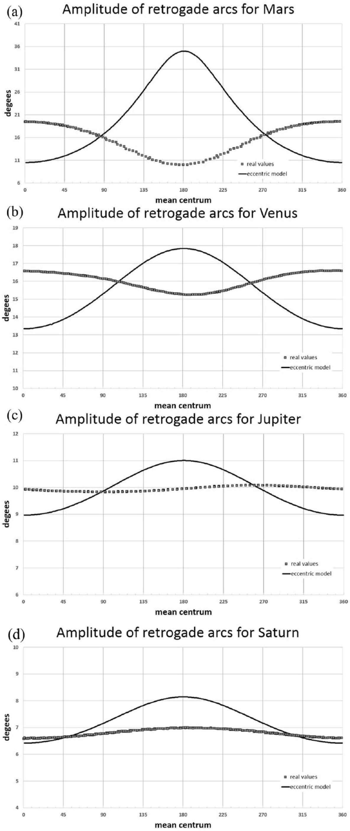
Graphs showing the amplitude of retrograde arc (real and according to the eccentric model) for (a) Mars, (b) Venus, (c) Jupiter, and (d) Saturn.
The difference between the predicted and the observed amplitudes for Mars is scandalous. In the case of the other three planets, this difference could also be detected even with a qualitative analysis of the observations: it would be enough to know that in Venus, the amplitude is somewhat smaller at perigee than at apogee, and that in Jupiter and Saturn, they are the same to realize that a concentric-with-epicycle model with the apogee and perigee fixed for predicting correctly the mean oppositions could not predict the amplitude of the retrograde arcs correctly for any planet. Therefore, this model requires the introduction of some major reformation.
The discovery of the equant point
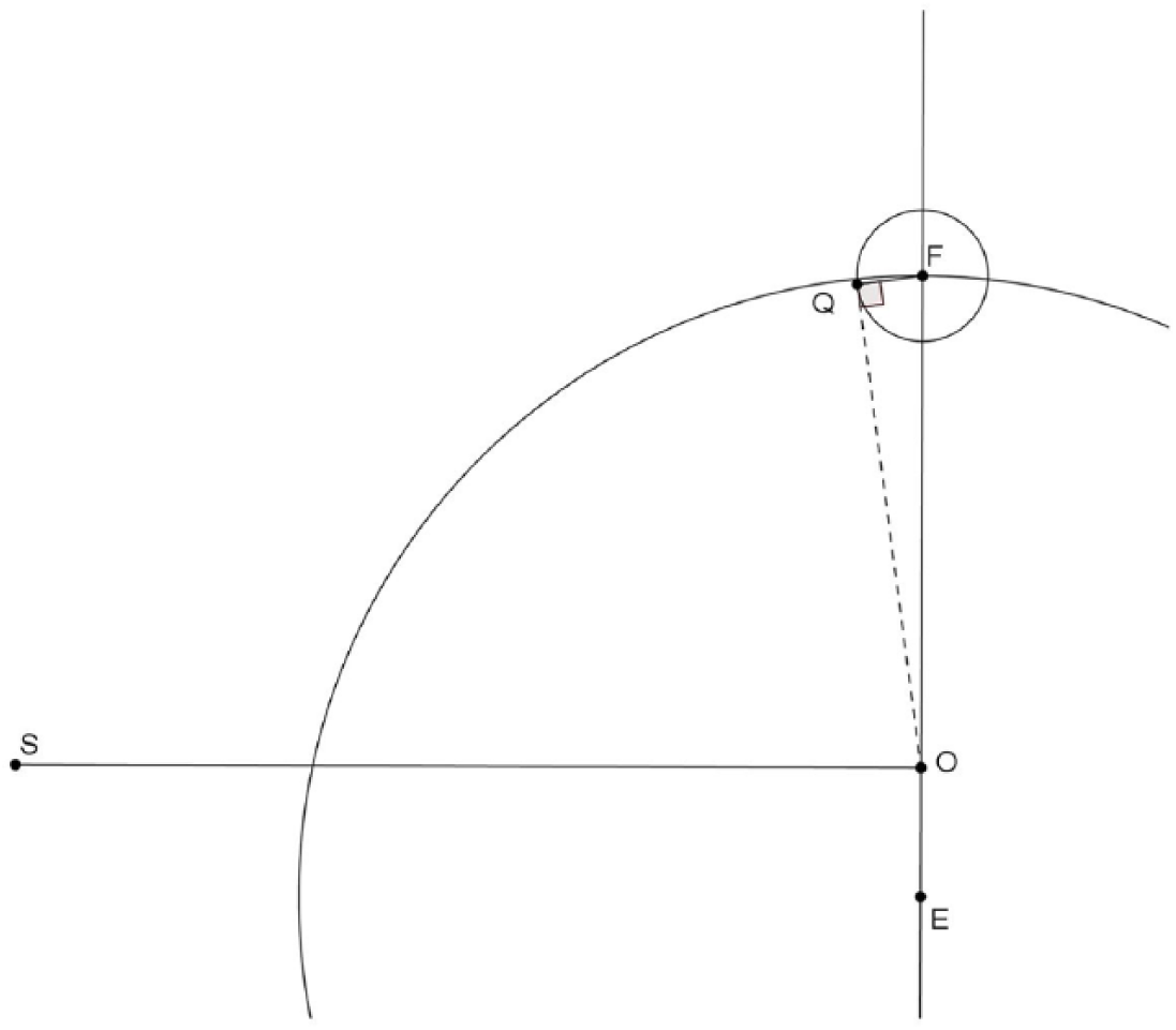
Once the impossibility of accounting for the phenomena using an epicyclic hypothesis – even one with an eccentric deferent – had been demonstrated, Ptolemy faced the hard task of coming up with a novel solution to the planetary problem. Figure 3 shows how this problem could have been formulated using only one retrogradation.
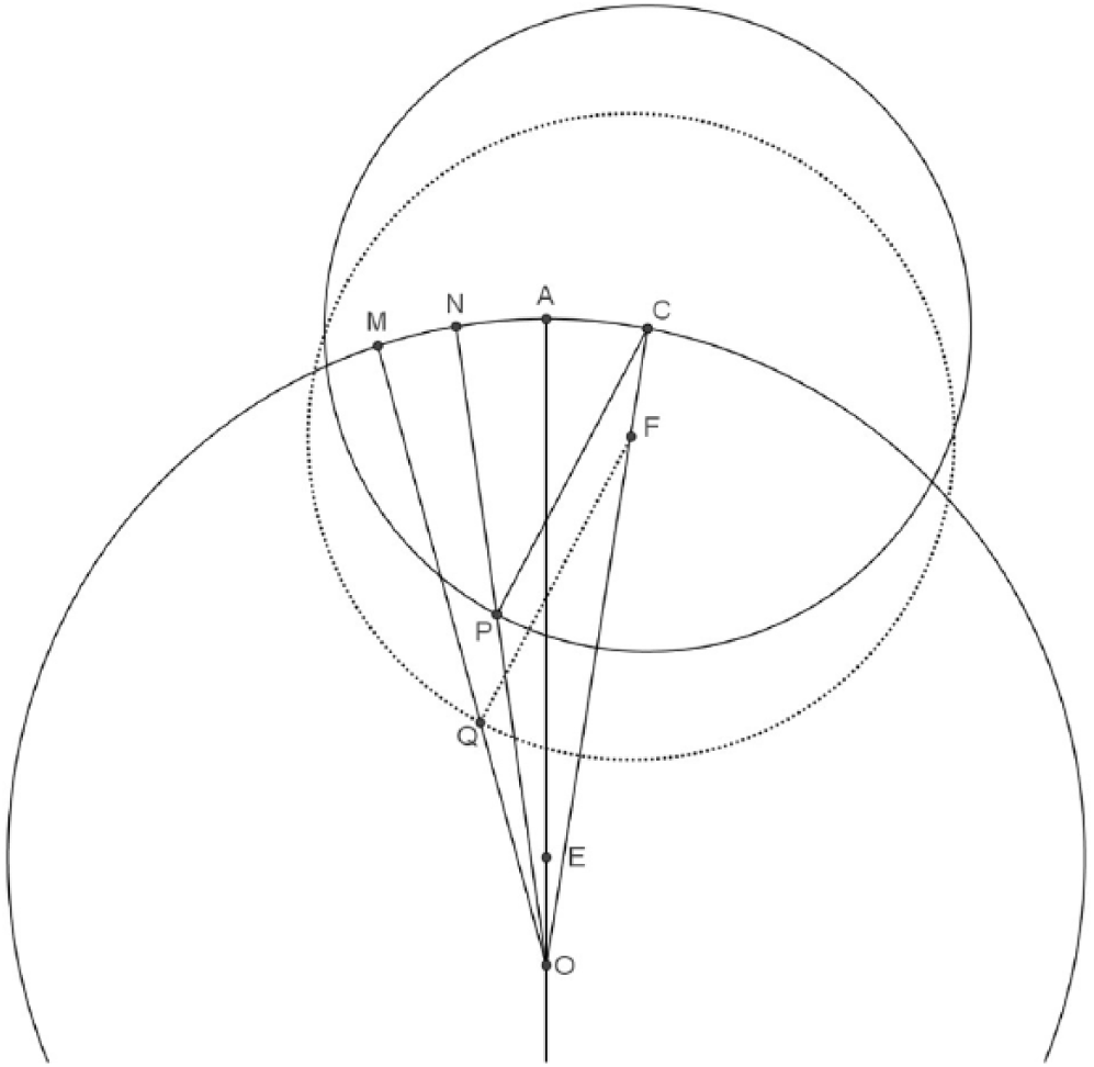
Discovery of the equant using one retrogradation at apogee. O is the centre of the ecliptic, and E is the centre of uniform motion and of the deferent. The apsidal line OEA has its apogee at A. P is the planet at the first station of a retrogradation whose mean opposition is at apogee. 17 Thus, the centre of the epicycle C has not yet arrived to A. ∠POC and ∠AOC represent apparent velocities in anomaly and in longitude, respectively, and are given from mean velocities and eccentricity OE.
The eccentric model predicts that half of the retrogradation will be equal to ∠AON, but, as we have shown, it is in fact greater, say equal to ∠AOM. Thus, the true location of the planet has to be on line OM. Now, ∠OCP and ∠AOC come from mean velocities and the eccentricity OE. The velocities, which are known to be correct, were obtained via the relations of planetary cycles. The eccentricity, which was also known to be correct, was obtained via the method of the three mean oppositions. In fact, those features of the model are responsible for its accuracy in predicting mean oppositions. So, whatever the corrections the model must undergo, these angles cannot be changed. The proportion R/r cannot be changed either, for it would equally affect the accuracy of the model.
Given these constraints, there is one plausible move in order to locate the correct position of both the planet and the centre of the epicycle: a new epicycle radius must be determined so that the extreme at which the planet is located touches line OM – i.e., at the observed true longitude – and the extreme at which the centre of the epicycle is located lies in line OC – i.e., at the calculated mean longitude. One would probably like to keep the size of the epicycle constant. Given the constraints introduced, this new epicycle must be equal and parallel to CP. Therefore, the correct position of the planet is at Q and not at P, and the correct centre of the epicycle is not at C, but at F.
This, of course, raises a serious problem: how can the centre of the epicycle be at F, if the circumference of the deferent lies further away from F? We cannot make the deferent smaller (making R = EF) because one constraint is keeping the proportion R/r. So, the only possibility seems to be moving the centre of the deferent E closer to the observer O along line OA, keeping the magnitude of R equal to CE, but leaving F lying in the circumference of the deferent. This move would entail, however, changing the eccentricity OE, which is responsible for the success of the model in predicting mean oppositions.
This is the Gordian knot that Ptolemy faced. His solution was a truly Alexandrian one.
Ptolemy could have realized that E must be moved inasmuch as it was the centre of the deferent, but at the same time that it could not be moved inasmuch as it was the centre of uniform velocity. So he decided to fulfil both demands, leaving the centre of uniform velocity at E, and moving the centre of the deferent towards the observer so as to account for the observed retrograde arc. This distinction is the heart of Ptolemy’s solution, and it signified the birth of the equant.
How much should the centre of the deferent move? The answer to this question required the introduction of some observed values into the calculation.
The discovery of the bisection of the eccentricity
If the same approach is used for calculating the approximate position of the eccentric point, the resulting values are really close to the bisection. The method is very simple and, assuming all of the parameters of the eccentric-with-epicycle model – r, R, 2e, and the mean velocities – it only requires one observational datum: the value of the amplitude of the retrograde is at apogee. As in Figure 1, make a diagram representing the model at the moment of the predicted first stationary point when the mean opposition takes place at the apogee. For example, in Figure 4, according to the model, the planet would be at P when it is seen stationary from O. Draw a line representing the line of sight of the position of the planet at the stationary point according to observation – dashed line OM in the diagram. While the model predicts that the planet would be seen at P when stationary, it is observed at line OQ. Because the eccentric model predicts the moment of the stationary point reasonably well, it is not necessary to observe the planet at the exact moment in which the model predicts the stationary point: one could simply take the known value for the retrograde arc at apogee for each planet. The mean positions of the planet and the epicycle are correctly measured from E, the eccentric point, as well as the proportion R/r. Therefore, one has to locate the planet in line OM, without changing angles AEC – mean centrum – and ECP – mean anomaly, the position of E, and the sizes of r or R. As we said, one should locate the planet at Q and the centre of the epicycle at F so that CFQP form a parallelogram. One has to look, therefore, for a new centre of the deferent in the apsidal line, but at distance CE from F. For this, draw an arc close to the apsidal line, centred at F and with radius equal to OC – the dashed arc in the figure. The intersection of the dashed arc and the apsidal line is the new centre of the deferent. Therefore, while the centre of uniform motion remains at E, the centre of the deferent must be moved to this new location in order to predict the observed amplitude of the retrograde arc correctly.

Mars during the first stationary point according to the eccentric-with-epicycle model. E is the centre of uniform motion and of the deferent. O is the observer. C is the centre of the epicycle at the moment of the first stationary point. The mean opposition will be reached when the centre of the epicycle, A, is in the apsidal line OA. The planet is seen stationary from O along the dashed line OM. To see it along line OM, the planet must be located at Q, the centre of the epicycle at F and the centre of the deferent in the intersection of the dashed arc and the apsidal line. The region close to the bisection is zoomed in the box on the lower right corner. The small dotted arcs in the zoomed area show the limits of the position of the centre of the deferent allowing an error of ±10′ in the determination of the longitude of the planet of the stationary point.
Figure 4 represents the situation for Mars, taking the values for R, r, and 2e from the Ptolemaic model for Mars. The values correspond to 38 days before the mean opposition at apogee: mean centrum = 340.08°, mean anomaly = 162.46°, half of retrograde arc according to model = 5.52°, and half of retrograde arc observed = 10°. The figure shows that the new centre of the deferent is impressively close to the bisection of the eccentricity, represented by point D. Allowing an error in the determination of half the retrograde arc of ±10 minutes 18 still gives values impressively close to bisection.
This method also works well for the other planets, assuming Ptolemy’s values for R, r, and 2e. The case of Venus is represented in Figure 5. The values correspond to 20 days before the mean opposition at apogee. Mean centrum = 339.3°, mean anomaly = 167.05°, half of retrograde arc according to model = 6.8°, and half of retrograde arc observed = 8.3°.

Venus during the first stationary point according to the eccentric-with-epicycle model. E is the centre of uniform motion and of the deferent. O is the observer. C is the centre of the epicycle at the moment of the first stationary point. The mean opposition will be reached when the centre of the epicycle, A, is in the apsidal line OA. The planet is seen stationary from O along the dashed line OM. To see it along line OM, the planet must be located at Q, the centre of the epicycle at F and the centre of the deferent in the intersection of the dashed arc and the apsidal line. The region close to the bisection is zoomed in the box on the lower right corner. The small dotted arcs in the zoomed area show the limits of the position of the centre of the deferent allowing an error of ±10′ in the determination of the longitude of the planet of the stationary point.
In the case of Jupiter, the values correspond to 61 days before the mean opposition at apogee (see Figure 6). Mean centrum = 354.93°, mean anomaly = 124.95°, half of retrograde arc according to model = 4.48°, and half of retrograde arc observed = 5°. Again, the new centre of the deferent is very close to the bisection.

Jupiter during the first stationary point according to the eccentric-with-epicycle model. E is the centre of uniform motion and of the deferent. O is the observer. C is the centre of the epicycle at the moment of the first stationary point. The mean opposition will be reached when the centre of the epicycle, A, is in the apsidal line OA. The planet is seen stationary from O along the dashed line OM. To see it along line OM, the planet must be located at Q, the centre of the epicycle at F and the centre of the deferent in the intersection of the dashed arc and the apsidal line. The region close to the bisection is zoomed in the box on the lower right corner. The small dotted arcs in the zoomed area show the limits of the position of the centre of the deferent allowing an error of ±10′ in the determination of the longitude of the planet of the stationary point.
In the case of Saturn, the values correspond to 70 days before the mean opposition at apogee (see Figure 7). Mean centrum = 357.66°, mean anomaly = 113.35°, half of retrograde arc according to model = 3.2°, and half of retrograde arc observed = 3.4°. This is the average between the maximum and the minimum amplitude of retrograde arc, assuming that Ptolemy wanted to produce a model in which there is no variation in the retrograde arcs like that of Jupiter. The position of the predicted centre of the deferent is not as good as in the other cases. In part, this is due to the fact that, being ∠OCP almost right, a very small variation of the amplitude observed implies big changes in the position of the new centre. The reason of the inaccuracy could also be due to the fact that Ptolemy’s value for the radius of the epicycle is fairly inaccurate, larger than what would be expected. For example, if we assume 3.5° for the observed half-amplitude, instead of 3.4°, the match is much better (see Figure 8). Of course, 3.4° could perfectly be rounded to 3.5°, but it is not necessary to suppose a value so close to the bisection for Saturn. The previous value, together with the results of the other planets, will be more than enough for affirming, as Ptolemy does, that […] in the case of each of these planets, speaking in terms of a rather rough method, the eccentricity that is found by means of the greatest difference caused by the zodiacal anomaly proves to be approximately double the eccentricity derived from the magnitude of the retrogradations around the greatest and least distances of the epicycle.
19

Saturn during the first stationary point according to the eccentric-with-epicycle model. E is the centre of uniform motion and of the deferent. O is the observer. C is the centre of the epicycle at the moment of the first stationary point. The mean opposition will be reached when the centre of the epicycle, A, is in the apsidal line OA. The planet is seen stationary from O along the dashed line OM. To see it along line OM, the planet must be located at Q, the centre of the epicycle at F and the centre of the deferent in the intersection of the dashed arc and the apsidal line. The region close to the bisection is zoomed in the box on the lower right corner. The observed amplitude of half the retrograde arc is 3.4°

Saturn during the first stationary point according to the eccentric-with-epicycle model. E is the centre of uniform motion and of the deferent. O is the observer. C is the centre of the epicycle at the moment of the first stationary point. The mean opposition will be reached when the centre of the epicycle, A, is in the apsidal line OA. The planet is seen stationary from O along the dashed line OM. To see it along line OM, the planet must be located at Q, the centre of the epicycle at F and the centre of the deferent in the intersection of the dashed arc and the apsidal line. The observed amplitude of half the retrograde arc is 3.5°. The region close to the bisection is zoomed in the box on the lower right corner. The small dotted arcs in the zoomed area show the limits of the position of the centre of the deferent allowing an error of ±10′ in the determination of the longitude of the planet of the stationary point.
The square and compass method applied to the Moon
We pointed out in the “Introduction” section that the equant is also present in Ptolemy’s second lunar model. As we said, Ptolemy indicates that, to account for the second lunar anomaly, he decided to include a moving centre of the deferent that does not coincide with the centre of uniform velocity. While Ptolemy does not explain which particular observations were used to devise his second lunar model and only refers to some data that serve as a mere corroboration of the theory, he does offer, in some detail, the results of the analysis he performed in order to achieve success. It is worth to quote Ptolemy in full here: When this type of observation was made without further analysis, it was found, both from the observations recorded by Hipparchus and from our own, that the distance of the moon from the sun was sometimes in agreement with that calculated from the above [simple] hypothesis, and sometimes in disagreement, the discrepancy being at some times small and at other times great. But when we paid more attention to the circumstances of the anomaly in question, and examined it more carefully over a continuous period, we discovered that at conjunction and opposition the discrepancy [between observation and calculation] is either imperceptible or small, the difference being of a size explicable by lunar parallax; at both quadratures, however, furthermore, at either quadrature, when the first anomaly is substractive the moon’s observed position is at an even smaller longitude than that calculated by substracting the equation of the first anomaly, but when the first anomaly is additive its true position is even greater and the size of this discrepancy is closely related to the size of the equation of the first anomaly.
20
This is the result of Ptolemy’s analysis. The newly discovered second anomaly is one that directly depends on the size and direction of the first anomaly, and also on the closeness of the epicycle’s centre to quadrature. Ptolemy does not provide a hint of how he came up with the solution to this problem. Right after this description of the anomaly, he continues, “From these circumstances alone we could see that we must suppose the moon’s epicycle to be carried on an eccentric circle, being farthest from the earth at conjunction and opposition, and nearest to the earth at both quadratures.” As one can see, there is no clue as to what sort of analysis he performed on the presumed observations, and, more importantly to our subject, how he came to the model he describes.
The method we proposed for obtaining the bisection of the eccentricity for the planets can also be successfully applied to the case of the Moon. Given Figure 9, Ptolemy knows that the Moon must be located on line OM and that the centre of the epicycle must be located on line OC. To preserve the success of the first model, mean velocities must remain untouched and so should the positions in mean longitude and mean anomaly. Thus, applying the method we described, Ptolemy could have determined an epicycle radius QF parallel to PC, where Q lies on line OM, and F on line OC. This would indicate that the centre of the deferent lies on point D, where DF is equal to OC, i.e., to 60 parts.
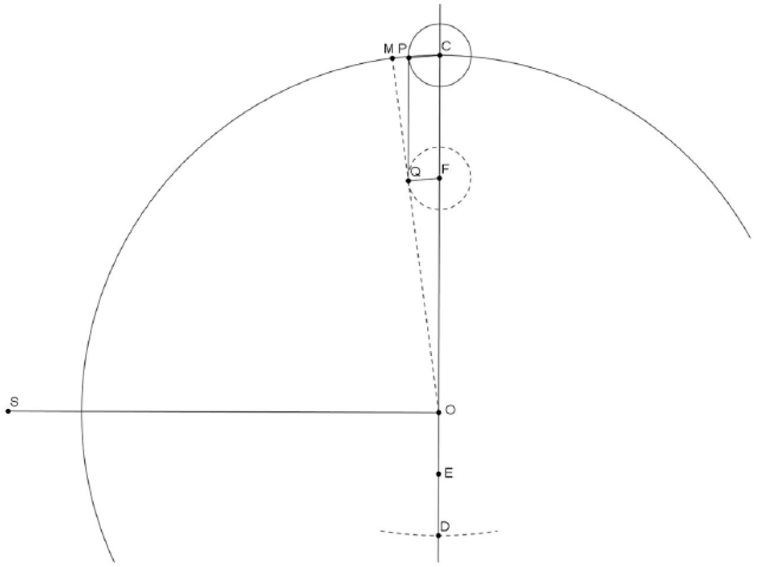
The method for finding the location of the equant applied to a lunar quadrature. Point O is both the centre of the ecliptic and of the deferent. The centre C of the epicycle is at quadrature from the mean Sun S, and the equation of the first anomaly is at its maximum, with the predicted Moon at point P. Observations, nevertheless, show that the Moon is not located at the longitude of P but at that of M. This shows that the model must be modified.
At this stage, the difference between the planetary models and that of the Moon comes into play: in the case of the Moon, the maximum and minimum anomalies are not fixed, but they depend on elongation. Given that, as Ptolemy stated, the first model was successful at syzygies, the distance from the observer to the centre of the epicycle at syzygies had to be equal to OC. Nevertheless, as this method would have been able to show, that distance had to be equal to OF at quadratures. In order to produce that effect, Ptolemy made the centre of the deferent move in a circle. The moving centre of the deferent should have an eccentricity which, when added to the distance from the observer to the centre of the epicycle, would yield a distance equal to OC. And, when subtracted to it, the eccentricity would yield a distance equal to OF. The simplest way to do this is to bisect OD with a new point E and to assume that this is in fact the centre of the deferent at quadrature. This results in a circle with radius OE (see Figure 10), where E moves in such a way that it lies on the segment OC at syzygies and on the opposite side – like in the diagram – at quadratures.
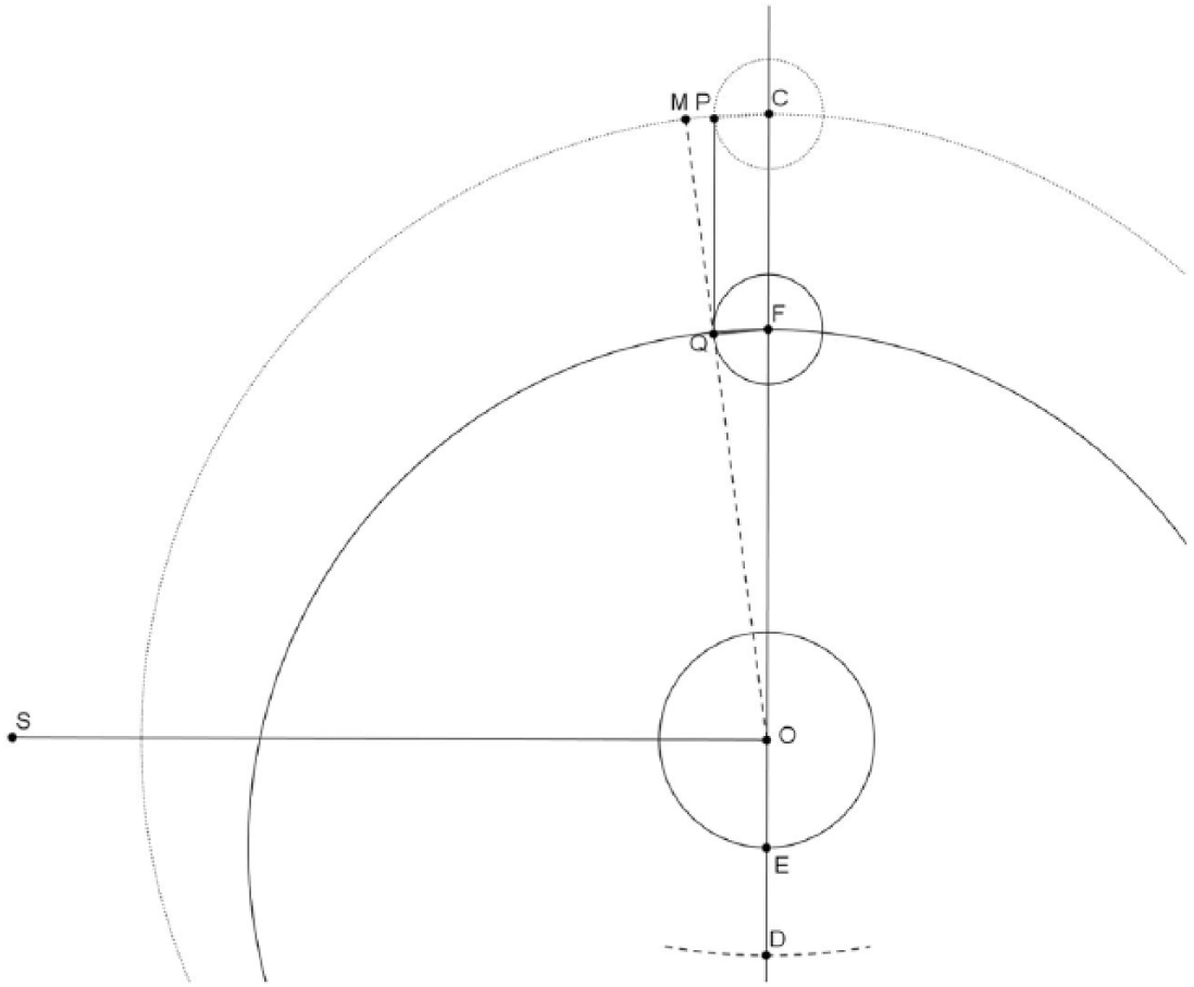
The second lunar model with a moving eccentric.
This method is very similar to the geometrical path that Ptolemy presents in V 4 to arrive to the parameters of the second lunar model. There is only one minor difference. In our method, the diagram represents the moment in which the first lunar model predicts the maximum anomaly, i.e., that the Moon moves at its mean velocity. Because the mean longitude and mean anomaly do not change between the first model and the second model, the angles representing the mean positions do not change either. Consequently, line CP is parallel to line FQ. Nevertheless, while P is the tangent point of the epicycle centred at C, Q is not the tangent point of the epicycle centred at F. This means that ∠FOQ is not the maximum anomaly and that the Moon, now at Q, is not moving at exactly its mean velocity. In other words, the second model does change not only the size of the anomaly but also the moment of the maximum anomaly. Ptolemy seems to be aware of this because when he describes the observational pattern that led him to the second lunar model, he says that the discrepancy between the first model and the observation “[…] reaches a maximum when the moon is near its mean speed and [thus] the equation of the first anomaly is also a maximum.” 21
Something similar happens when the method is applied to the planetary models: the diagram represents the moment of the stationary point that the first model predicted – eccentric without equant, but, once the centre of the deferent is moved, the moment of the stationary point changes as well. The longitude of the planet does not change significantly close to the stationary point; therefore, it is perfectly reasonable to assume that the planet is still stationary at this moment. Besides, because the method represents the same moment, all mean motion angles can be kept. This constitutes the main reason of the simplicity of the method. Thus, it is very convenient to represent the situation of both models in the moment of the first stationary point of the first model in the case of the planets.
On the contrary, in the case of the Moon, it is not necessary to represent the moment of the maximum anomaly according to the first model in order to know the mean motion angles (see Figure 11). Because at maximum anomaly ∠FQO is right and ∠FQO is known, the angle of the mean anomaly, ∠QFO, is also known. By also knowing the radius of the epicycle, FQ, Ptolemy can calculate distance FO. In this case, therefore, the method does not require the preservation of the moment of the maximum anomaly according to the first model in order to know the relevant angles. This is what Ptolemy did in V 4.
The method for calculating the parameters of the second model offered in the Almagest (V, 4; H1 365–366; 225–226).
Leaving aside this minor difference, however, the method is similar: in both cases, we are trying to obtain the distance between the observer and the centre of the epicycle at which the apparent size of the epicycle will be observed, knowing the mean anomaly, the mean longitude, and the size of the epicycle. Moreover, the method is applied in both cases to the apogee of the epicycle with a resulting epicycle closer to the observer. Finally, in both cases, the phenomenon used for calculating the correct distance of the epicycle centre is related to a particular velocity of the body: in the case of the Moon, its mean speed, and in the case of the planets, when the speed is null.
The square and compass method applied to the planets, using maximum equations of anomaly
It is interesting to ask, however, if there is any way through which Ptolemy could have found the eccentricity of a planet’s centre of the deferent using maximum equations of anomaly instead of stationary points. There is, of course, the case of Venus, in which Ptolemy describes
22
a method that heavily relies on maximum elongations, which only happen at the moments when the equation of anomaly is at its maximum. Thus, in this case, the maximum elongation is a mean to finding the maximum equation of anomaly. Could one follow the same method with the outer planets? Ptolemy’s answer is explicitly negative: However, the demonstrations by which we calculate the amounts of both anomalies and apogees cannot proceed along the same lines for these planets as for the previous two [Mercury and Venus], since these [the superior planets] reach every possible elongation from the sun, and it is not obvious from observation, as it was from the greatest elongation for Mercury and Venus, when the planet is at the point where the line of our sight is tangent to the epicycle. So, since that approach is not available, we have used observations of their oppositions to the mean position of the sun […].
23
The method he uses is the one that relies on three mean oppositions, which we mentioned above.
It is important to note, though, that the method of the three oppositions relies on a geometrical relation between the line joining the centre of the epicycle and the planet, and the line joining the Earth and the mean Sun: given the fact that “for each of these [superior] planets, the sum of the mean motions in longitude and anomaly […] equals the motion of the sun […],” 24 it happens that the lines to which we referred “[…] will always be parallel to each other […].” 25 It follows, then, that both lines will effectively coincide at the moment of mean opposition, thus allowing the astronomer to determine the position of the centre of the epicycle. There is, however, another synodic configuration which is derived from this geometrical relation, one through which an astronomer could have easily determined the moment of maximum equation of anomaly.
In Figure 12, the elongation of the planet and the mean Sun – ∠SOP – is 90°. Given that OS // EP, then OP ⊥ EP, and thus ∠EPO is also 90°. But ∠EPO can only be a right angle if P is located at the point where our line of sight is tangent to the epicycle, i.e., when the planet’s equation of anomaly is at maximum. In this simple way, Ptolemy could have located the moment of maximum equation of anomaly of a superior planet, by looking for the moment of a mean elongation of 90° – a synodic method which relies on the same foundations as the one he uses for finding the centre of uniform velocity. Therefore, when a planet is exactly at quadrature with respect to the mean Sun – something which could be easily calculated – it is at its maximum equation of anomaly, and the method that Ptolemy used for the Moon could be applied in exactly the same way. In the case of Mars, the difference in the equation of anomaly predicted by the eccentric-with-epicycle model and the observed one is, in the perigee, 8.37°. Therefore, the method could be perfectly applied. Unfortunately, however, this method cannot be successfully applied to Jupiter and Saturn, for their eccentricities and radii of epicycles are too small, and therefore, the difference between the predicted equations of anomaly and the observed ones is barely perceptible even at perigee – where the maximum difference takes place: 0.59° for Jupiter and 0.43° for Saturn.
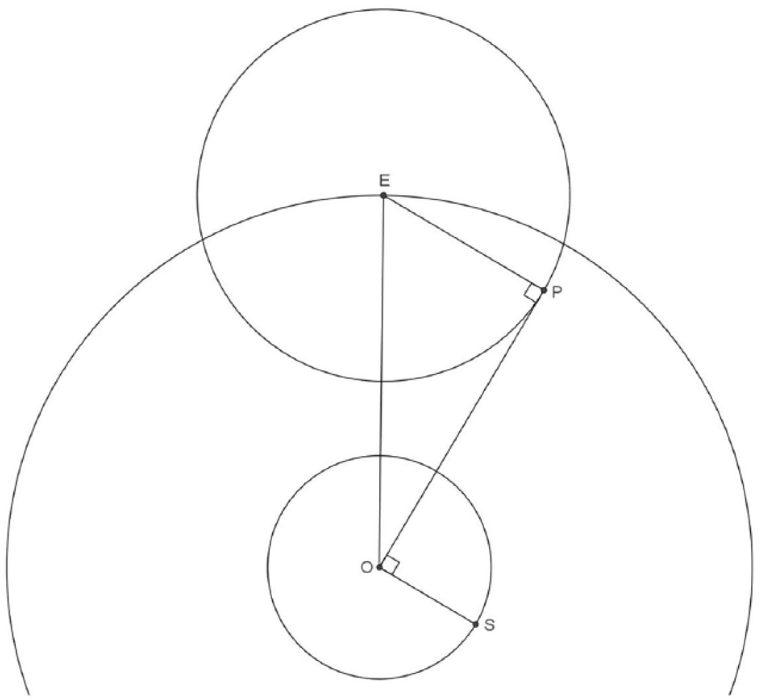
Maximum equation of anomaly of an outer planet. Point S is the mean Sun, with a deferent concentric with the observer at O. The centre of the epicycle is E, with the planet at P.
This method is curiously similar to that advanced by Jones, who suggests using what Pliny calls nonagenarii or nintieths to find the eccentricity of the centre of the deferent. A nintieth refers to the moment in which Mars is at an elongation of 90° from the Sun, which takes place roughly 90 days after and before the mean opposition. Neugebauer interpreted that the nonagenarii refer to the points when Mars passes in direct motion through the longitude of its opposition that roughly occurs close to the quadrature with respect to the Sun. 26 Jones builds his argument in this aspect of the nonagenarii, leaving aside the fact that their elongation is approximately 90°. Nevertheless, it is possible to build an argument based on the elongation feature of the nonagenarii. In Figure 13, we present two different situations: in the first one, the planet is at M when the centre of the epicycle is at A, the apogee. The equation of anomaly is at its maximum, and the elongation from the mean Sun, at T, is 90°. In the second one, the planet is at N when the centre of the epicycle is at P, the perigee. The equation of anomaly is at its maximum and the elongation from the mean Sun, at N, is 90°. Now, the equation of anomaly in the first case, represented by ∠AOM, is 43°, while in the second, represented by ∠POM, is around 53.25°. The distance from the observer to the centre of the epicycles is easy to obtain from these two angles, and the eccentricity for the centre of the deferent, D, is very close to 6.
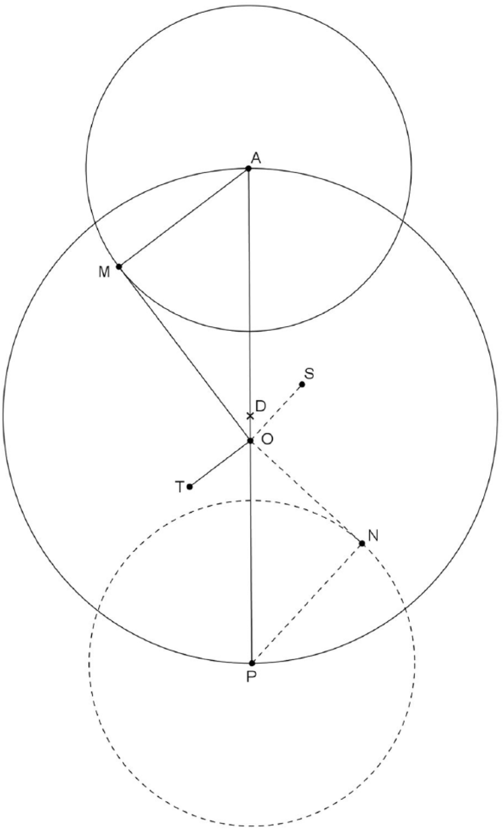
Mars’ eccentricity of the centre of the deferent and the nonagenarii.
The direction of influence between the lunar and planetary equant models
It seems clear to us, then, that both the planetary and lunar equants are answers to a more general phenomenon that can be treated with a single method. If this is the case, both discussions related to the equant point in the planets and in the Moon would be mutually enriched if studied together. It seems reasonable to suppose, then, that the solution of the planetary problem influenced the solution of the lunar problem, or the other way around. Knowing, however, which one influenced the other is a rather difficult question, for which we probably do not have enough evidence to pose a final answer.
The introduction of the equant point in the lunar model is in book V, and those of the planets in books IX and X, but, of course, this order does not imply anything, for the order of the books is related to the general structure of the Almagest. Moreover, no conclusion can be obtained from the date of the observations used for illustrating the different models in the Almagest. Nevertheless, something might be inferred by comparing the way Ptolemy describes his discovery of the second lunar model in the above-quoted passage and the way he introduces the equant point for the planetary models.
Thoroughly considering the text in which Ptolemy introduces the second lunar model, 27 one can see that he devotes very little space to the exposition of the model itself, and none to the way he discovered it. Most of it is devoted to the exposition of the results of the analysis he performed on lunar observations, i.e., the exposition of how he found a pattern of behaviour in a very complex mass of observational data. The emphasis he puts on this aspect of his research could be seen as a sign that Ptolemy considered that the big breakthrough in his lunar investigation was not the invention of a model with an equant, but the discovery of the fact that the lunar problem was just another case of an already treated – and solved – difficulty. In addition, he seems to say that the model follows immediately from these patterns of behaviour when he introduces the model. Ptolemy usually uses the first person of the plural, so it is hard to distinguish when he is talking about himself and when he is using the “we” in a more didactical way, involving him and the reader. A. Jones, however, noted (personal communication, Sept. 2017) that Ptolemy uses past tense verbs when he is talking about his own discoveries, while he uses the present tense when he wants to express something in a more didactical approach. Therefore, when Ptolemy says, talking about the discovery of the pattern of behaviour of the anomaly, “[…] we paid more attention […] and examined, […] we discovered […],” he is talking about his own research and investigation and it is almost certain that Ptolemy is attributing to himself the discovery of the pattern that will be explained with a moving eccenter. Nevertheless, when he says “[…] from this pattern of behaviour [of the lunar anomaly] we can see immediately that it must be assumed that the Moon’s epicycle too travels on an eccentric circle,” 28 he returns to the didactical “we.” It is clear, therefore, that Ptolemy emphasizes that he discovered the pattern of the behaviour, but he is not emphasizing that he discovered the model.
Moreover, when he says that “[…] the point of the above remarks was not to boast [of our own achievement] […]” 29 after discussing why Hipparchus could have not proposed any planetary model before starting the description of the equant model for the planets, he offers some sort of justification of why he had to introduce a procedure not in strict accordance with the theory. So it seems that, here, he is talking of his own invention. Of course, this does not mean that Ptolemy discovered the equant point, but he might have discovered an aspect of it, such as the bisection. Nevertheless, the way Ptolemy approaches the description of both models could be an indication of the influence of the planetary solution on the lunar problem, leaving the question open on whether Ptolemy, or one of his predecessors, discovered the equant solution for the planets.
Footnotes
Acknowledgements
We want to thank Alexander Jones, Dennis Duke, Anibal Szapiro, Diego Pelegrin, and Gustavo Zelioli for their comments and suggestions of earlier versions of this paper. We also would like to thank Daryn Lehoux’s and Nathan Sidoli’s comments, both of whom attended a conference in which we presented this paper, the Fourth International Workshop on Epistemology and Astronomy, July, Rio de Janeiro, Brazil.
Funding
We would like to express our thanks for the support of Research Projects PICT-2014-1741, PICT-2014-0775, and PICT-2016-4487 of the Agencia Nacional de Promoción Científica y Tecnológica of Argentina.