Hipparchos and the ancient analemma

Introduction

In his Commentary on the Phenomena of Aratos and Eudoxos, Hipparchos tells us that he showed how to produce numerical values for three phenomena related to the star υ Boö (Upsilon Boötis) “by means of lines” (διὰ   τῶν γραμμῶν) in what he calls “our systematic treatises” (In Arat. II.2.25–28), ¹ which may be a reference to his treatise on simultaneous risings explicitly mentioned in the previous passage (In Arat. II.2.24), or perhaps to general works on mathematical methods for spherical astronomy. In particular, when υ Boö is on the western horizon, he is able to state (Problem 1) the right ascension of its parallel at the midheaven, (Problem 2) the degree of the ecliptic at the midheaven, and (Problem 3) the degree of the ecliptic on the eastern horizon. In 1900, H.G. Zeuthen pointed out that expressions related to διὰ τῶν  γραμμῶν in both Ptolemy’s Almagest and his Analemma indicate solutions through exact geometric methods, especially through chord-table trigonometry, and showed, in a general way, that the values that Hipparchos states could be computed through such methods, although he did not give many of the details for the computations related to υ Boö. ² This understanding of διὰ τῶν γραμμῶν was then fleshed out by P. Luckey in his study of Ptolemy’s Analemma and its mathematical methods. ³ Indeed, Ptolemy seems to use διὰ  τῶν γραμμῶν as a technical expression for chord-table trigonometry, and there is reason to believe that before him Hipparchos did as well. ⁴

Following this, G. Toomer and O. Neugebauer showed in detail how plane chord-table trigonometry could be used on an analemma figure to compute the value found in Problem 1, the right ascension at the midheaven. ⁵ In 2004, I demonstrated how the so-called Sector, or Menelaus, Theorem, could be used to compute the values for Problem 2 and Problem 3, and argued, incorrectly, that an analemma diagram could not be used for these purposes. ⁶ Recently, E. Landi and F. Schironi have shown that Problems 2 and 3 can be solved using solid geometry. ⁷ In this paper, I show in full detail how the analemma methods can indeed be used to compute all three problems.

Using the analemma to model the celestial sphere

In this section, I introduce the terminology that I will use to discuss spherical astronomy, much of which is standard, and explain how the analemma figure can be used to model the celestial sphere. The ancient analemma methods are particularly suited to, and were probably developed for, describing the fundamental relationships of spherical astronomy.

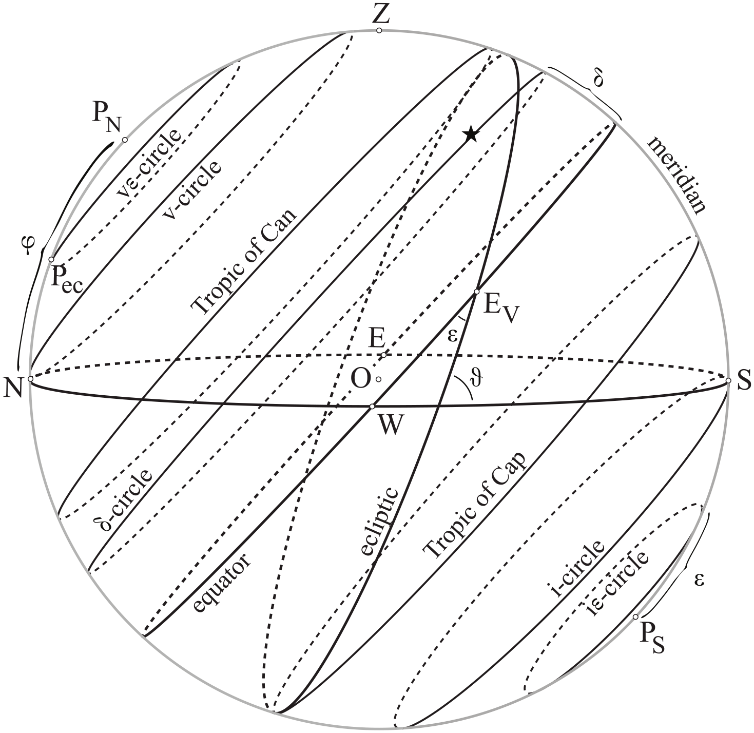
In Figure 1 the observer, O, is assumed to be a point in the center of the celestial sphere, which rotates uniformly over the course of a stellar day, around axis P_NP_S (not shown in Figure 1) joining the north and south poles, points P_N and P_S. In his Commentary, Hipparchos sets the latitude of Rhodes to be φ : = 36 ° (In Arat. I.11.8). This determines the orientation of the local horizon, gC(NESW), relative to the celestial axis P_NP_S. The other principal great circles of the local coordinate system are the meridian, g C ( S Z P N N ) —which passes through the north point, N, the south point, S and the zenith, Z—and the prime vertical (not shown)—which passes through the east point, E, the west point, W, and Z. Any point of the celestial sphere, or a star fixed on it, can be stated in terms of an angle around the horizon, and the great-arc distance between the point and the horizon, measured along a great circle passing through Z and the nadir (not shown).

OPEN IN VIEWER

Figure 1.

The celestial sphere. The sphere rotates uniformly from E to W around axis P_NP_S, so that a given star ★ is carried on a circle of constant declination, its δ -circle, throughout the course of a stellar day. The vernal equinox, E_V, will soon set over the western horizon, which faces the viewer. Throughout the course of the year, the sun advances along the ecliptic in the opposite direction (from W to E), measured from E_V as the start of the cycle, λ : = 0 ° . Points on the equator, and the δ -circles, are measured in the same general direction and from the same starting point E_V, α : = 0 ° . Not to scale.

The celestial equator is the greatest circle of a bundle of parallel circles that we can call δ -circles, because they all have constant declinations. Since the ecliptic is fixed in the celestial sphere, it forms with the equator an angle known as the obliquity of the ecliptic, ε , and the two great circles intersect at two diametrically opposite points, the vernal equinox, E_V, and the autumnal equinox (not shown, on the back of the diagram). The other principal great circles of the equatorial coordinates are the equinoctial colure (not shown), passing through E_V, P_N, E_A (not shown), and P_S, and the solstitial colure (not shown), passing through the poles and points separated by 90° from the equinoxes along the equator (or the ecliptic).

As the sphere rotates, for all terrestrial latitudes besides the equator and the poles, some stars will always be visible above the horizon, and circle about the visible pole; other stars will never appear; and the middle band of stars will rise over the eastern horizon (back of the diagram) and set over western horizon (toward the viewer), returning to the same location in one stellar day. We can call the greatest small circle of the ever-visible stars the v -circle and that of the ever-invisible stars the i-circle. These visibility circles are the two small circles that are parallel to the equator and tangent to the horizon. ¹² Any given star—say ★ in the upper righthand portion of the diagram—is carried about a circle of constant declination—its δ -circle, which ancient texts sometimes call a day circle. ¹³

Because the equator and δ -circles are determined by the motion of the celestial sphere, they have a fixed angle with the horizon, φ ′ = 90 ° − φ . As the sphere rotates, however, the ecliptic will make a regular wobbling motion relative to the horizon throughout the course of a stellar day. In particular, (1) its angle with the horizon, say ϑ , will be greatest when E_V coincides with the west point W, least when it coincides with the east point E, and will vary symmetrically and monotonically on either side of these extremes, and (2) its pole will orbit the celestial pole on a small circle whose great-arc radius is equal to ε . ¹⁴ We can call this circle the v ε -circle, because if we lived at a location such that φ : = ε , this would be our v -circle. Moreover, the pole of the ecliptic, say P_ec, is fixed in the celestial sphere—such that where E V : = α = 0 ∘ the right ascension of P_ec is 270° —and hence it moves about its circle at the same speed and in the same direction as the motion of the whole. Thus, when it is known what point of the equator is on the meridian, the arc of the v ε -circle from the meridian to P_ec is also known.

It is well known that the ancient analemma was used to model the instantaneous position of the sun in local coordinates, for the purposes of making sundials and solving various problems in spherical astronomy, such as we find in Vitruvius’ Architecture IX.7, Heron’s Dioptra 35, and Ptolemy’s Analemma. ¹⁵ In fact, however, the analemma model can also be used to address many problems in spherical astronomy that do not involve the position of the sun. As a first example of the use of the analemma to model stellar phenomena, we may consider a given star rising over the horizon at a given location. Considering Figure 2, we may describe some star, ★, rising or setting on the local horizon. In this configuration, the analemma, or receiving, plane is that of the meridian, the analemma circle is the meridian gC(NP_NZS), with N the north point, Z the zenith, and S the south point. The celestial axis lies in the meridian such that P_N is the north pole, elevated over the horizon at an angle equal to that of the terrestrial latitude, φ . Then, star ★ will be carried on a δ -circle throughout the day whose diameter we may call AB. Hence, at the moment of rising (or setting), the star will be on the normal to plane of the analemma (here the meridian), which lies in the plane of the horizon. Hence, the distance between the star and the plane of the analemma is an upright, u₁, to the drawing of the analemma—which drawing is in a plane parallel to the actual horizon, but not necessarily to the horizon as depicted in the diagram. We should understand u 1 to be a distance, or a numerical measure of a distance, which may be represented by various geometrical segments in the diagram—such as P_RC in Figure 2. Then, if we draw the δ -circle directly in the plane of the analemma, as though folded on its diameter, the rising point of the star will be P_R, and the common section of the horizon and the star’s δ -circle will be P R C = u 1 , which represents the perpendicular dropped from the star to the plane of the meridian. Then, throughout a stellar day, the star rises at P_R, moves up to cross the meridian at A, moves back down to set at P_R, and then moves on to cross the meridian below the horizon at B, finally returning again to P_R. All of this takes place on a δ -circle whose great-arc distance from the equator is measured by arc δ of the meridian. Notice that the magnitudes of all lines and arcs in this diagram are preserved, so that any computation of these elements in the analemma figure will result in a computation of the corresponding spherical elements.

OPEN IN VIEWER

Figure 2.

Analemma diagram of a star rising (or setting) on the horizon at a given terrestrial latitude ψ.

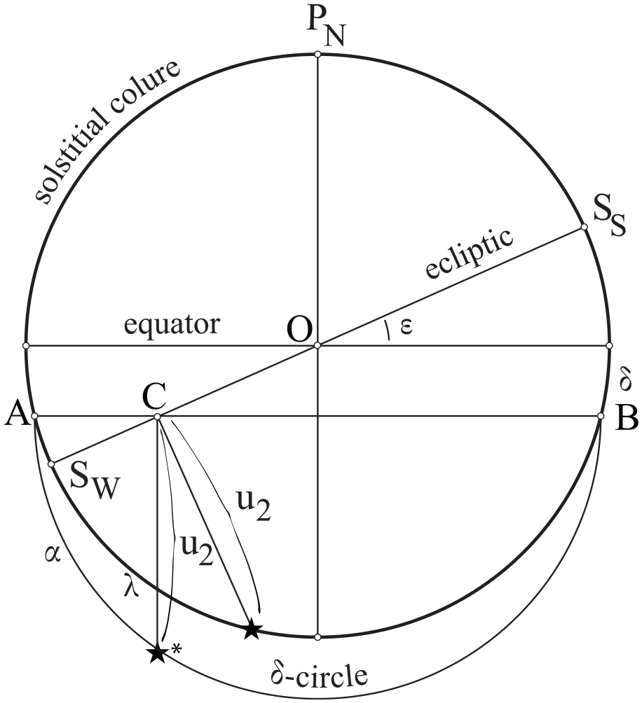
It is not necessary that the analemma plane represent the meridian. In our second example, by making a different choice, we can show how to exhibit a star on the ecliptic in both ecliptic and equinoctial coordinates. Considering Figure 3, we set the analemma plane as that of the solstitial colure and the analemma circle as the colure itself, gC(S_S P_N S_W), with S_S as the summer solstice, P_N as the north pole, and S_W as the winter solstice. Then, the diameter of the equator will be perpendicular to the celestial axis, and the diameter of the ecliptic will meet the solstitial colure at points S_S and S_W separated from the equator by a great-arc distance equal to the obliquity of the ecliptic, ε . If we consider the ecliptic folded into the plane of the analemma along their common section, it will coincide with the analemma circle. Since the longitudes of the solstices are known (90° for S_S and 270° for S_W), the longitude of a star on the ecliptic, ★, can be measured off as λ . Since the star is on the ecliptic, it has no ecliptic latitude, β = 0 ∘ . Then, throughout a day, the star, ★*, will be carried on a δ -circle with diameter AB whose great-arc distance from the equator is measured on the analemma circle by δ along the colure. Furthermore, since the upright from the star itself, ★ and ★*, to the plane of the solstitial colure is u 2 , a segment dropped from the star perpendicular to the plane of the analemma will be the common section of the ecliptic and the δ -circle of ★. If we draw the δ -circle folded into the plane of the analemma along its diameter AB, then the segment ★*C = u₂ will determine the star’s position on the δ -circle and cut an arc α as measured from 90°, the right ascention at the colure. Note, once again, that all elements drawn in this diagram preserve their relative magnitudes in both the solid and analemma configurations.

OPEN IN VIEWER

Figure 3.

Analemma diagram of star on the ecliptic as exhibited in both ecliptic ( λ , 0°) and equinoctial coordinates ( α , δ ).

As we will see below, the fact that the star is represented as a different point in the two different coordinate systems, ★ and ★*, while the upright u 2 is the same distance, and therefore represented by segments of equal length in both, is essential to using the analemma model as a computational tool. It is possible to prove that ★C and ★*C must be equal in a number of different ways. For example, we could use plane geometry to show that they must be equal in the plane of the analemma, and then use a solid argument similar to that in Ptolemy’s Analemma 6 to show that they each represent the segment between the star and the plane of the analemma. ¹⁶ The simplest argument, however, probably comes from considering the analemma construction itself. Namely, since u 2 is the distance between the star and the plane of the analemma, by the definition of a line perpendicular to a plane, Elem. XI.def.3, the perpendicular segment dropped from the star into the plane of the analemma must be perpendicular to any line through the foot of the segment, C, such as the diameters of the circles, S_WCS_S and ACB.

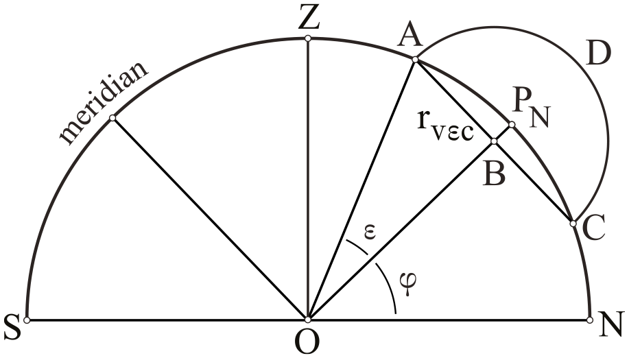
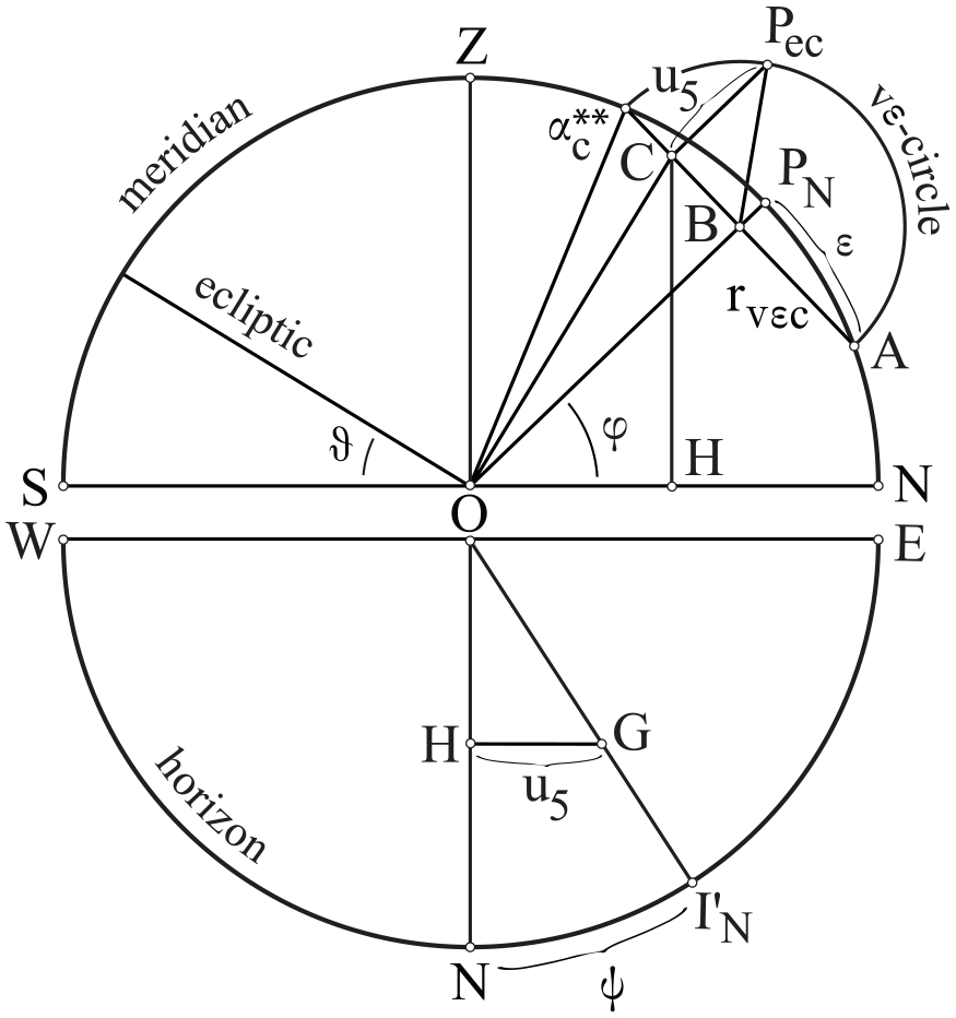
Finally, we can show how the analemma model can be used determine the elements of the v ε -circle, on which the pole of the ecliptic, P_ec, is carried throughout the course of a day. In Figure 4, we set the half of the analemma circle semiC(NZS) as the local meridian; ∠ N O P N : = φ as the terrestrial latitude, or elevation of the pole; and semiC(ADC) as the circle on which pole P_ec is carried, drawn directly in the analemma plane.

OPEN IN VIEWER

Figure 4.

Analemma diagram of the circle of the pole of the ecliptic, the vε-circle. Not to scale.

Then, as the ecliptic is carried with the celestial sphere in its daily rotation, P_ec will move on semiC(ADC) at the same angular velocity, and in the same direction as the whole. In particular, it will cross the meridian toward the zenith at point A, and travel along semiC(ADC) to cross the meridian again toward the north point at C, and then head back again to A. Since this motion is fixed to that of the cosmos, if the right ascension at either A or C is given, then the position of P_ec on semiC(ADC) will be given. Furthermore, since the obliquity of the ecliptic is given, ε G , where we assume the radius of the cosmos, R = O A , as some value, R _G , the chord table allows us to assert the ratio of the radius of the vε-circle, say r _vεc , to R—namely,

( r v ε c : R ) G .

(by CT) (0.1)

Hence, if we state some value for the radius of the analemma circle, we can state a value for r v ε c in this base. Furthermore, by Elem. I.47, the ratios of all the sides of rightT(ABO) can be stated pairwise. For example, the distance of the circle of P_ec from the center of the sphere can be stated in relation to the radius of the sphere,

( O B : R ) G .

(by Elem. I.47) (0.2)

Use of the analemma to solve Hipparchos’ three problems

In this section, I will introduce the numerical values that Hipparchos assumes as well as those that he claims to have computed, and then show how the analemma methods can be used to solve each of the three problems that he states. I will show in a general way how to compute the values that he says he computed using the values that he says he started with for all three problems, but I will only give an example computation for Problem 1.

Overview of the three problems

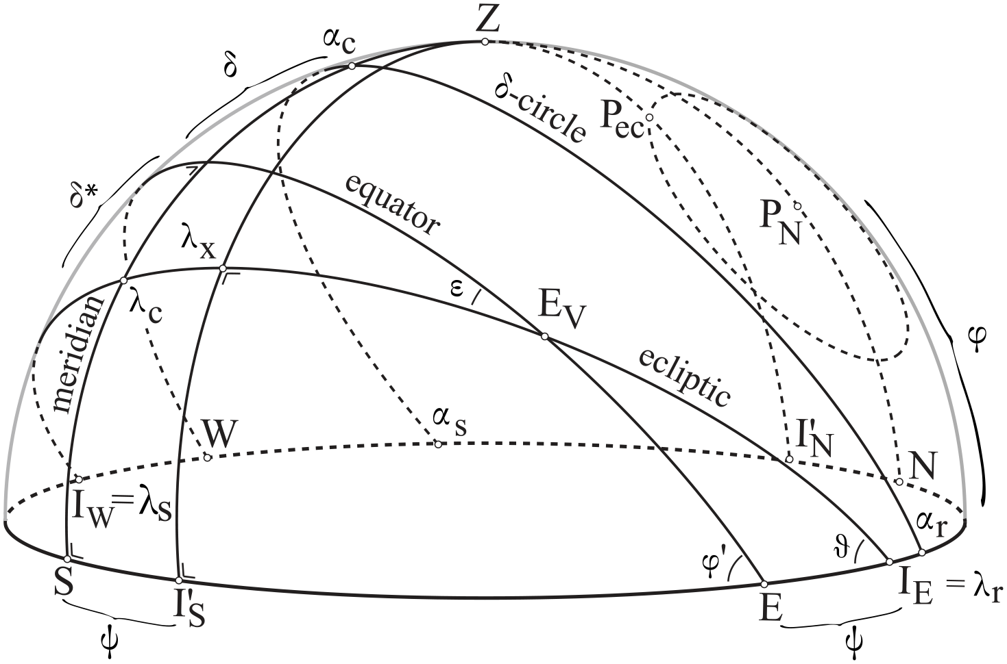
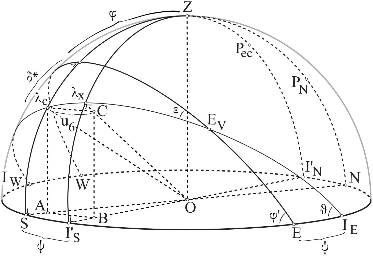
In order to understand the overall configuration described by Hipparchos in these passages, we can refer to a perspective diagram of the hemisphere above the horizon when υ Boö stands on the western horizon. In Figure 5, we consider horizon gC(NWSE), with zenith Z, and set the celestial pole P_N at φ : = 36 ° above horizon, such that the meridian passes through points N, P_N, Z, and S. Since υ Boö is at δ = 27 1 2 ° N, its δ -circle will be just north of the Tropic of Cancer (not shown), and the right ascension of υ Boö, α : = 181 ° , will be setting on the western horizon, at point α s . The δ -circle of the star will be culminating at the meridian at α c and will be rising on the eastern horizon at α r .

OPEN IN VIEWER

Figure 5.

Perspective diagram of the hemisphere above the horizon when υ Boö is on the western horizon, as described by Hipparchos. Not to scale.

In Problem 1, Hipparchos calculates A r c ( α s α c α r ) = 224 1 4 ° , and estimates A r c ( α s α c ) ≈ 112 1 2 ° , so that the right ascension of point α c is 293 1 2 ∘ .

In Problem 2, Hipparchos uses the right ascension of α c to compute the degree of the ecliptic, λ c , that is culminating when υ Boö stands on the western horizon. He states a longitude of this point that is equivalent to λ c = 291 ° . We will see that this is closely related to a transformation of coordinates between the equatorial and the ecliptic coordinate systems. That is, if we consider the δ -circle (not shown) at an unknown declination δ * that passes through the unknown λ c at β = 0 ° , λ c will correspond to α = 293 1 2 ° on this δ -circle. We will see below that the same analemma figure that can be used to transform between coordinates can be used to find both λ c and δ * .

In Problem 3, λ c = 291 ∘ is used to compute the point of the ecliptic that is rising on the eastern horizon, λ r . Hipparchos states an equivalent to λ r = 35 ∘ . In order to find this point using the analemma, we can make a two-stage computation. First we use the analemma model to determine the instantaneous position of the ecliptic—namely the orientation and inclination of the ecliptic on the horizon circle when υ Boö stands on the western horizon. Namely, we will find the great-arc distance ψ between the two intersection points of the ecliptic with the horizon—I_E near E and I_W near W—and E and W respectively. This angle will be the same as the great-arc distance between the intersections of the vertical circle passing through P_ec and Z, g C ( I ′ N P e c Z I ′ S ) , with the horizon— I ′ N near N and I ′ E near S—and N and S respectively. Using the same geometric configuration, we can determine the dihedral angle ϑ that the ecliptic makes with the horizon, such that the great-arc distance, measured along the vertical g C ( I ′ N P e c Z I ′ S ) between I ′ S on the horizon and λ x on the ecliptic is ϑ . The second stage of this problem can be solved using the analemma model in a least two ways. (1) We can use three different analemma diagrams to find the perpendicular from point λ c to the plane of vertical g C ( I ′ N P e c Z I ′ S ) , from which we can compute A r c ( λ c λ x ) of the ecliptic. (2) Alternatively, we can use a single analemma diagram, comparable to that used in Problem 2, to find A r c ( λ c λ x ) . Then, since point λ x is the midpoint of the semicircle of the ecliptic above the horizon—namely, A r c ( λ s λ x ) = A r c ( λ x λ r ) = 90 ° —the value of λ x will allow us to state that of λ r .

Problem 1

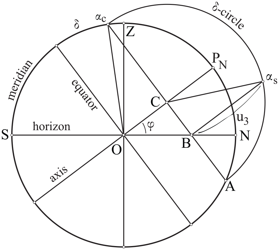
An analemma solution to this problem is extensively covered in the literature. ²⁰ The diagram is essentially the same as those used in Ptolemy’s Analemma. Here we will first go through how the computation can be summarized using metrical analysis, and then follow through with a numerical computation using a hypothetical chord table that is sometimes attributed to Hipparchos.

In Figure 6, we set the analemma circle gC(NP_NZS) as the meridian, with the radius of the cosmos as O Z = R , and we assume that we can state the values for the declination of υ Boö, as δ G , and the terrestrial latitude, as φ G , which are, at least in principle, observationally determined.

OPEN IN VIEWER

Figure 6.

Analemma diagram for Problem 1. Not to scale.

Then, in r i g h t T ( O C α c ) the acute angle at α c is A n g ( O α c C ) G = δ G , so we can state

( O C : R ) G , and

(1.1a)

( α c C : R ) G .

(both by CT) (1.2a)

Likewise, since we can state φ G , in rightT(OCB), we have values for

( O C : C B ) G ,

(by CT) (1.3a)

hence,

( C B : R ) G .

(by Data 8) (1.4a)

But, B α c = α c C + C B , B A = α c C − C B , and R ( B α c , B A ) = S ( B α s ) = S ( u 3 ) , by Elem. III.35, so we can state

( C B : u 3 ) G , that is ( C B : B α s ) G .

(by Data 8) (1.5a)

Hence, in r i g h t T ( C B α s ) , we can compute the value for

A n g ( α s C B ) G .

(by CT) (1.6a)

Hence, the arc of the δ -circle of υ Boö above the horizon is 360 ° − 2 A n g ( α s C B ) G , and A r c ( α s α c ) G is half this value.

Next, we will follow through the same argument using numerical computations involving a chord table and the various computational rules corresponding to the propositions of Euclid’s works cited above. It must be acknowledged that such an exercise is fairly arbitrary, since we know the details of neither Hipparchos’s chord table, nor his methods of calculation. Nevertheless, this numerical example may help some readers see how the metrical analysis summarized above corresponds to an actual calculation. For these purposes, I will assume standard linear interpolation on a chord table of 7 1 2 ∘ steps and a base diameter of 6875^p arbitrary parts, such as is attributed to Hipparchos by a number of modern scholars. ²¹ I will, however, use sexagesimal fractions, despite the fact that I believe Hipparchos did his computations using Egyptian, or unit, fractions. This is because computations involving Egyptian fractions make use of auxiliary tables, and we do not know what tables Hipparchos may have used. (Readers who have no interest in the details of chord-table trigonometry can skip ahead to the end of this section.)

In Figure 6, we know that A n g ( O α c C ) G = δ G : = 27 1 3 ° = 27 ; 20 60 ° , and setting the radius of the circle to be the diameter of our chord table, R = O α c : = 6875 p , and since angles standing on the same chord at the center of a circle are twice those on the circumference, we can enter with both 54 ; 40 ° = 2 × 27 ; 20 ° and 125 ; 20 ° = 180 ° − 54 ; 40 ° into the chord table to find

3168 ; 58 , 40 p : 6875 p = ( O C : R ) G , and

(1.1b)

6104 ; 45 , 20 p : 6875 p = ( α c C : R ) G .

(1.2b)

Furthermore, since φ G : = 36 ° , if we set the hypothenuse of r i g h t T ( O C B ) to be the diameter of the chord table, we can enter into the chord table with both 72 ° = 2 × 36 ° and 108 ° = 180 ° − 72 ° to find the chords of OC and CB when O B : = 6875 p . That is,

5559 ; 48 p : 4039 ; 36 p = ( O C : C B ) G ,

(1.3b)

We can then use the rule-of-three with the values in (1.3b) and (1.1b) to compute C B = 3168 ; 58 , 40 p × 4039 ; 36 p ÷ 5559 ; 48 p = 2302 ; 29 , 36 p in terms of R : = 6875 p , so that

2302 ; 29 , 36 p : 6875 p = ( C B : R ) G .

(1.4b)

But since all these values are in terms of R : = 6875 p , we can compute

B A = α c C − C B = 6104 ; 45 , 20 p − 2302 ; 29 , 36 p = 3802 ; 15 , 43 p ,

and

B α c = α c C + C B = 6104 ; 45 , 20 p + 2302 ; 29 , 36 p = 8407 ; 14 , 56 p .

And, by the property of secants lines in a circle,

B α s = u 3 = 3802 ; 15 , 43 p × 8407 ; 14 , 56 p = 5653 ; 53 , 53 p ,

so that,

2302 ; 29 , 36 p : 5653 ; 53 , 53 p = ( C B : B α s ) G .

(1.5b)

In this way, we know the legs of r i g h t T ( C B α s ) when R : = 6875 p , so that its hypothenuse can be computed as

C α s = 2302 ; 29 , 36 p 2 + 5653 ; 53 , 53 p 2 = 6104 ; 45 , 20 p .

Then, still in r i g h t T ( C B α s ) , setting C α s : = 6875 p and using the rule-of-three we can find

B α s = 5653 ; 53 , 53 p × 6875 p ÷ 6104 ; 45 , 20 p = 6367 ; 15 , 27 p

in the same parts, so that we can enter into the chord table to compute the angle subtending chord B α s as 135;43,10°. Hence,

67 ; 51 , 35 ° = 135 ; 43 , 10 ° ÷ 2 = A n g ( α s C B ) G .

(1.6b)

Hence, the arc of the δ -circle of υ Boö above the horizon is 360° − 135;43,10°  =  224;16,49°. The value that Hipparchos states for this arc is equivalent to 224;15°. Since we do not know the details of Hipparchos’ computation procedures, nor even what geometrical model he used, I think a discrepancy of 0;1,49₆₀° ≈ 0.03₁₀° after all these calculations is fairly low. ²²

Problem 2

For this problem, we are seeking the value in longitude of the point of the ecliptic that stands at the midheaven, λ c , given that we know the value of the right ascension of all δ -circles at the midheaven, α c G . Back in Figure 5, if we consider the position of point λ c in both equatorial and ecliptic coordinates, we know its right ascension, α c G , but not its declination, and we know its ecliptic latitude, β = 0 ° , but not its longitude λ c . Hence, it should be obvious in principle that, since two alternate coordinates in each pair of coordinates for the same point are fixed, the two other coordinates are also fixed. In a moment, we will rehearse a non-rigorous argument that this is the case based on the analemma diagram.

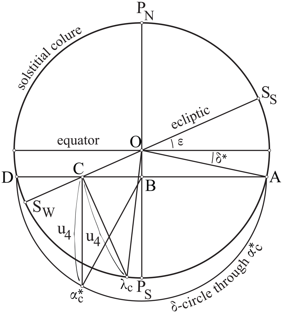
In order to compute the longitude and declination of point λ c we will use an analemma diagram in which the analemma circle is set as the solstitial colure. The general configuration is the same as those used by Ptolemy in his Analemma for points on the ecliptic, with the exception that he always sets the analemma circle to be the meridian. In Figure 7, with the equator arranged horizontally, P N is the north pole at the top and P S is the south pole at the bottom, so that the ecliptic is inclined at a given angle ε G to the equator. Hence, the δ -circle passing through λ c will stand on diameter A B C D at some unknown declination, δ * , toward the south. The point λ c on the sphere will be mapped to both λ c along the ecliptic and to some point, say α c * , on the δ -circle, such that A r c ( D α c * ) G = α c G − 270 ∘ , is the δ -circle-arc distance of the meridian from the solstitial colure. In this way, u 4 = C α c * ⊥ A B C D is the upright from α c * , which is a mapping of λ c , to the colure. Finally, on the ecliptic point λ c will stand upright from the colure at the same linear distance, u 4 = C λ c ⊥ S S O C S W , so that we seek A r c ( S W λ c ) = λ c − 270 ° as the longitude of λ c .

OPEN IN VIEWER

Figure 7.

Analemma diagram for Problem 2. Not to scale.

Considering the analemma diagram, Figure 7, in which A r c ( D α c * ) G and ε G are given, it should be clear that if the ecliptic latitude is fixed, say β = 0 ° , then point λ c will also be fixed. This can be seen from the fact that as point D, on A B C D ∥ equator , varies between the equator and point S W , A n g ( D B α c * ) will vary between approaching 0° as D approaches S W and approaching 90° as D approaches the equator—and similarly on the other side of the equator. Thus, if point α c * is fixed, so must be point C, and hence also point λ c .

We can give a summary of the computation of the position of λ c as follows. Since A n g ( D B α c * ) G = α c G − 270 ° , then in r i g h t T ( C α c * B ) ,

( C B : u 4 ) G , that is ( C B : C α c * ) G .

(by CT)

Likewise, since ε G is given, in r i g h t T ( C B O )

( O B : C O ) G , a n d

(2.1)

(CB : CO)G (both by CT)

so that

( C O : u 4 ) G , that is ( C O : C λ c ) G .

(by Data 8)

Hence, in r i g h t T ( C O λ c ) , we can compute a value for

A n g ( C O λ c ) G .

(by CT)

This gives us the value of the longitude as λ c G = 270 ° + A n g ( C O λ c ) G .

Since we will use this below in Problem 3.2, it should be shown that is also possible to compute δ * , the declination of point λ c , on the same analemma diagram. Indeed, in r i g h t T ( C O λ c ) , since we know ( C O : C λ c ) G while O λ c = R , we know

( C O : O λ c ) G , that is ( C O : R ) G .

(by Elem. I.47)

So, with (2.1), we know

( O B : R ) G , that is ( O B : O A ) G .

(by Data 8)

Hence, in r i g h t T ( A B O ) , we can compute the value of

δ G * = A n g ( O A B ) G .

(by CT) (2.2)

Problem 3

As mentioned above, in order to solve this problem we must first (3.1) determine the instantaneous position of the ecliptic, from which we can either (3.2a) determine the linear distance of λ c from the plane of the vertical great circle through P_ec and Z, g C ( I ′ N P e c Z I ′ S ) , or (3.2b) determine the arc of the ecliptic between λ c and λ x , the intersection of the ecliptic with g C ( I ′ N P e c Z I ′ S ) . In Problems 1, 2, 3.1, and 3.2b the analemma diagrams are similar to those in Ptolemy’s Analemma, but the analemma diagrams used for the final part of 3.1 and in 3.2a involve only great circles, and hence are different from most of those we find in ancient sources. Nevertheless, such diagrams are found in analemma constructions in classical and medieval Arabic sources.

Problem 3.1

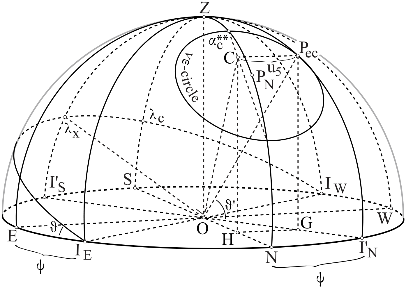
In order to determine the instantaneous position of the ecliptic, we need to locate the pole of the ecliptic P_ec relative to the local horizon at the moment when υ Boö is on the western horizon. In Figure 8, the v ε -circle, the δ -circle of pole P_ec, has a great-arc radius equal to A r c ( α c * * P N ) G = ε G , and small circle A r c ( α c * * P e c ) G = α c G − 270 ° ,since the right ascension of P_ec is 270°. Hence, the position of P_ec on the v ε -circle is known.

OPEN IN VIEWER

Figure 8.

A perspective diagram showing the pole of the ecliptic P_ec on the v ε -circle, and its relation to the instantaneous position of the ecliptic. Not to scale.

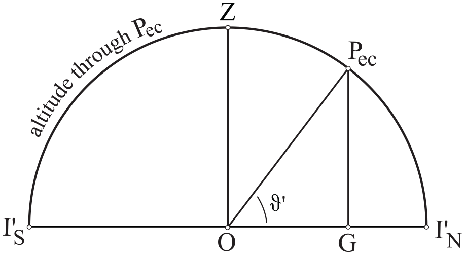
Furthermore, if we drop perpendiculars from P_ec to both the plane of the meridian, as P_ecC, and the horizon, as P_ecG, then the elements of Euclid’s solid books can be used to show that P_ecC will be perpendicular to the radius of the v ε -circle in the plane of the meridian at point C, and P e c G ⊥ O I ′ N at G. Hence, if we drop G H ⊥ O N , then G H ∥ P e c C , and the solid properties of R ( C P e c G H ) can be used to find the position of the ecliptic. Namely, (1) the relationship between O H and u 5 = G H = P e c C determines angle ψ  separating the endpoints of the diameter of the ecliptic in the horizon from those of the equator, and (2) the relationship between OG and O P e c determines ϑ ′ , the complement to ϑ .

These angles can both be computed using analemma methods. We begin, in Figure 9 (Top), by setting the analemma circle to be the meridian such that the celestial pole P_N stands above the horizon at φ G , and the pole of the ecliptic P_ec is located on the v ε -circle, which has an angular separation of ε G from P_N, such that the value of A r c ( α c * * P e c ) G = α c G − 270 ° is known. Furthermore, recall that we can compute the parameters of the v ε -circle relative to the sphere, namely we can state ( r v ε c : R ) G and ( O B : R ) G (see (0.1) and (0.2), p.8, above).

OPEN IN VIEWER

Figure 9.

Analemma diagrams for Problem 3.1a. In the top diagram the analemma circle is the meridian, while in the bottom diagram it is the horizon. In medieval works, such analemma diagrams are usually drawn in single circle; here separated for clarity. Not to scale.

Then, in r i g h t T ( P e c C B ) in which P e c B = r v ε c , since we know the value of A n g ( C B P e c ) G ,

( u 5 : r v ε c ) G , that is ( P e c C : r v ε c ) G , and ( C B : r v ε c ) G ,

(both by CT)

so, since we have ( r v ε c : R ) G by (0.1) above, we can state

( u 5 : R ) G , that is ( P e c C : R ) G , and

(3.1.1)

( C B : R ) G .

(both by Data 8)

Furthermore, with ( O B : R ) G by (0.2) above, we have

( C B : O B ) G ,

(by Data 8)

so that, in r i g h t T ( C B O ) , we can compute

A n g ( C O B ) G .

(by CT)

Hence, we can compute

A n g ( C O H ) G = A n g ( C O B ) G + φ G .

(by Data 3)

Likewise, in r i g h t T ( C B O ) we know

( C O : O B ) G ,

(by Elem. I.47)

so, with (0.2),

( C O : R ) G .

(by Data 8)

Hence, in r i g h t T ( C H O ) —since we already have ( u 5 : R ) G = ( P e c C : R ) G by (3.1.1)—we can fully state the parameters of the internal rectangle R ( P e c C H G ) relative to the sphere, namely

( C H : R ) G , and

(3.1.2)

( O H : R ) G .

(both by Data 8 and CT)

Now, in Figure 9 (Bottom), we set the analemma circle as the horizon, and consider the arrangement of the meridian and the vertical circle through P_ec, which are both perpendicular to the horizon. If we set ON as the radius of the meridian, and O I ′ N as the radius of the vertical circle through P_ec, then we can set out OH (Bottom) as ( O H : R ) G (Top) and erect G H ⊥ O N such that G H = P e c C = u 5 , where ( u 5 : R ) G , as above. Hence, we have

( O H : G H ) G ,

(by Data 8)

so that we can compute

( O G : R ) G ,

(by Elem. I.47) (3.1.3)

and also

Ψ G = A n g ( H O G ) G .

(by CT) (3.1.4)

Finally, we can compute the value of ϑ by considering r i g h t T ( O G P e c ) in the altitude circle that passes through P_ec in Figure 8. If we set the analemma circle as the altitude through P_ec, in Figure 10, using (3.1.3) and (3.1.2) we know both ( O G : R ) G and ( G P e c : R ) G = ( C H : R ) G , since G P e c = C H . Hence, we can compute the value of

ϑ ′ G = A n g ( G O P e c ) G ,

(by CT)

so that we have

ϑ G = 90 ∘ − ϑ ′ G .

(3.1.5)

In this way, we can compute the values of both ψ and ϑ G , so that the instantaneous position of the ecliptic is known numerically.

OPEN IN VIEWER

Figure 10.

Analemma diagram for Problem 3.1b. Computation of ϑ ′ . Not to scale.

Problem 3.2

Now, given the instantaneous position of the ecliptic, in Figure 11, we must determine the value of A r c ( λ c λ x ) , the great-arc distance between point λ c and point λ x , the intersection of the ecliptic with the vertical circle through P_ec, which is perpendicular to the ecliptic and along which the elevation of the ecliptic over the horizon is measured. We can do this in at least two different ways using analemma methods.

OPEN IN VIEWER

Figure 11.

Perspective diagram showing the orthogonal projection of point λ c onto both the horizon, at point A, and onto the vertical circle through λ x , which is perpendicular to the ecliptic, at point C. Not to scale.

The first approach to Problem 3.2, say 3.2a, is geometrically comparable that in Problem 3.1. If we drop perpendiculars from λ c to both the plane of the vertical through P e c , as λ c C , and the horizon, as λ c A , then it can be shown that λ c C will be perpendicular to the radius of the ecliptic through λ x , namely λ c C ⊥ O λ x at point C in the plane of the ecliptic, and λ c A ⊥ O S at point A in the plane of the meridian. Furthermore, if, in the plane of the horizon, we drop A B ⊥ O I ′ S , then λ c C ∥ A B , and we can use the properties of R ( λ c A B C ) , and in particular, line λ c C in the plane of the ecliptic, to calculate A r c ( λ c λ x ) .

A r c ( λ c λ x ) is computed using analemma diagrams in two steps: (1) first we find the linear height of λ c above the horizon, λ c A , and then (2) we find the linear distance of λ c from the vertical through P e c , namely λ c C .

First, in Figure 12 (Top), we set the analemma circle to be the meridian, such that N O S is the diameter of the horizon, Z is zenith, and point λ c lies on the southern arc of the meridian. Then, the arc from the zenith to λ c , say ζ , is that which Ptolemy calls the descendant (καταβατικóς, decensivus) in his Analemma. ²³ But, we can state the value of ζ , because it is equal to the great-arc distance between Z and the ecliptic, ψ G , and the declination δ G * , which we know from (2.2)—that is, we can state

ζ G = δ G * + φ G .

(by Data 3)

Hence, in r i g h t T ( λ c A O ) , we can state

( O A : λ c O ) G , that is ( O A : R ) G .

(by CT)

OPEN IN VIEWER

Figure 12.

Analemma diagrams for Problem 3.2a. Not to scale.

Next, in Figure 12 (Bottom), we set the analemma circle to be the horizon, such that NOS is the diameter of the meridian, and O I ′ S is the radius of the vertical circle through P e c , with an angular separation from the meridian of ψ G , as computed in (3.1.4). We lay off OA on NOS, where ( O A : R ) G . Then, if we drop u 6 = A B ⊥ O I ′ S , in r i g h t T ( O A B ) , we can state

( O A : A B ) G ,

(by CT)

so that

( u 6 : R ) G , that is ( A B : R ) G .

(by Data 8)

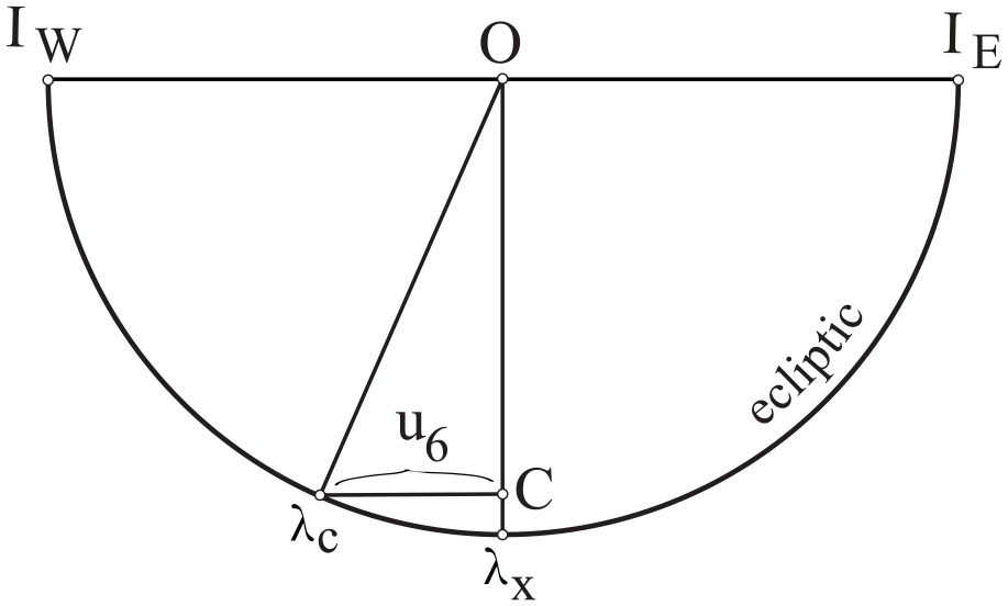
Finally, by setting the analemma circle as the ecliptic, in Figure 13, we can compute the value of A r c ( λ c λ x ) by considering r i g h t T ( O C λ c ) in the plane of the ecliptic, in Figure 11. Namely, in r i g h t T ( O C λ c ) , since we can state ( u 6 : R ) G , that is ( λ c C : R ) G , then we can calculate

A n g ( C O λ c ) G = A r c ( λ c λ x ) G .

(by CT)

Hence, since Arc (λ_x I_E)_G = 90°, we can state the value of

A r c ( λ c I E ) G = A r c ( λ c λ x ) G + A r c ( λ x I E ) G .

(by Data 3)

In this way, we can state the longitude of the ecliptic on the eastern horizon, as point I E = λ r G when υ Boö is setting, in Figures 5 and 11.

OPEN IN VIEWER

Figure 13.

Analemma diagram for the last step in Problem 3.2a. Not to scale.

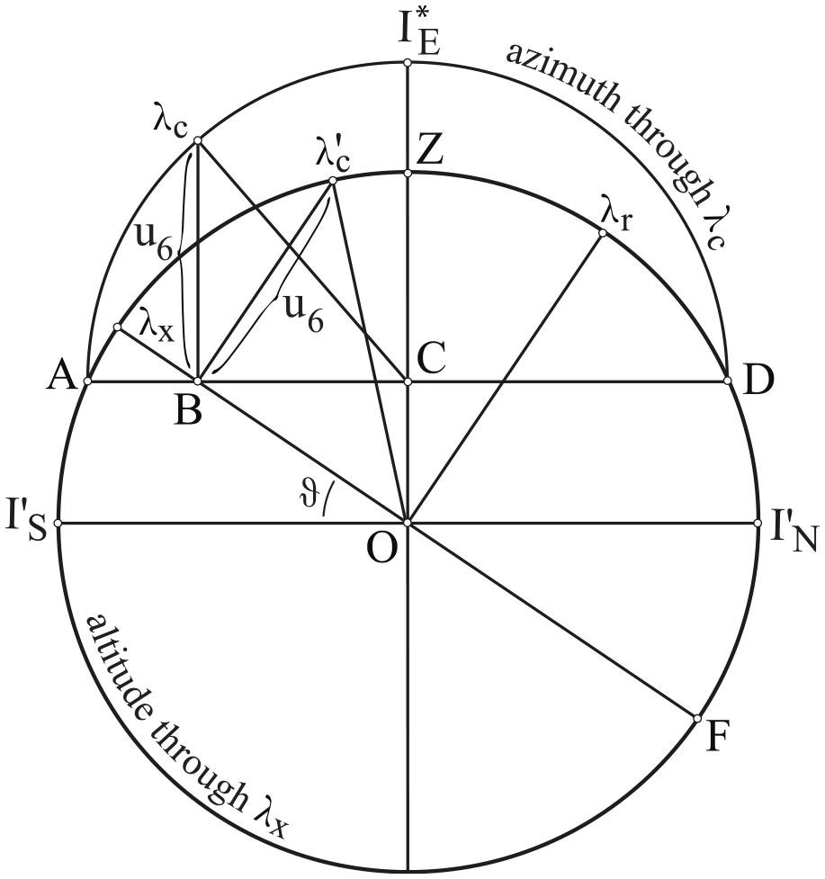
In fact, however, there is another solution to Problem 3.2, say 3.2b, which uses the fact that we know both ϑ G and A n g ( S I ′ S ) G = ψ_G in Figure 11, and models the problem as geometrically related to a transformation of coordinates and as equivalent to the solution to Problem 2. ²⁴ For this procedure, we will set the analemma circle as the altitude circle passing through λ x and consider the azimuth circle passing through λ c , which will be geometrically analogous to the δ -circle through α c * in Problem 2.

In this case, we consider the instantaneous position of the ecliptic relative to the horizon, such that the horizontal coordinates of azimuth and altitude play the same role here as the equatorial coordinates of right ascension and declination played in Problem 2. That is, in Figure 14, we set the analemma circle as the altitude circle passing through λ x , such that its diameter in the horizon is I ′ S I ′ N , and the ecliptic will be inclined toward the horizon at a dihedral angle equal to ϑ G , so that its diameter in the plane of the analemma is λ x O F . Hence, the azimuth circle through λ c , with diameter ABCD in the plane of the analemma, will pass through λ c at an unknown altitude above the horizon. The point λ c will be on this azimuth circle separated by an arc equal to ψ G from point A in the altitude circle passing through I ′ S . In this way, u 6 = λ c B ⊥ A B C D is the upright from λ c to the plane of the analemma. Finally, on the ecliptic λ ′ c will stand upright to the analemma at the same linear distance, u 6 = λ ′ c B ⊥ λ x B O F , so that we seek A r c ( λ x λ ′ c ) .

OPEN IN VIEWER

Figure 14.

Analemma diagram for Problem 3.2b. Not to scale.

We can summarize the analemma computation of A r c ( λ x λ ′ c ) as follows. Since A r c ( A λ c ) G = A n g ( B C λ c ) G = ψ_G, then in r i g h t T ( B C λ c )

( B C : u 6 ) G , that is ( B C : B λ c ) G .

(by CT)

Likewise, since ϑ G is given, in r i g h t T ( B C O )

( B C : B O ) G ,

(by CT)

so that we can state

( B O : u 6 ) G , that is ( B O : B λ ′ c ) G .

(by Data 8)

Hence, in r i g h t T ( B O λ ′ c ) , we can compute a value for

A n g ( B O λ ′ c ) G = A r c ( λ x λ ′ c ) G .

(by CT)

Then, once again, we can state the longitude of the ecliptic on either horizon when υ Boö is setting.

Conclusion

Having gone through these arguments one might well pose the question of whether or not we are now compelled to believe that Hipparchos actually calculated the numbers that he states using analemma methods. In fact, we do not know how Hipparchos proceeded. He may have used the analemma, but it is possible to compute the stated values using various different mathematical methods. For example, he could have used plane cord-table trigonometry on the geometrical construction of the planisphere, as described in Ptolemy’s eponymous text, and to which construction Hipparchos had some connection—at least, according to Synesios of Cyrene, writing around the turn of the fifth century. ²⁵ As mentioned above, it is also possible to do these calculations using solid geometry; and we find problems of spherical astronomy handled using solid geometry in the astronomical texts of medieval India. ²⁶ Furthermore, Hipparchos might also have used the spherical methods of the Sector Theorem, which involve simpler computations. ²⁷ The question of which one of these methods is the simplest, or most natural, is subjective, and would be answered differently depending on one’s own mathematical education and experience. We have no way of knowing what Hipparchos may have thought about such matters. ²⁸

Writing in the fourth century, Theon of Alexandria credited Hipparchos with a work on Chords (τῶν  ἐν  ϰύϰλῳ εὐϑειῶν) in 12 books, which is sometimes asserted to be much too long. ²⁹ This assertion, however, is based on the assumption that Hipparchos must have been doing the same thing in these 12 books that Ptolemy is doing in the half book in which the latter introduces his chord table. But this assumption is not necessary. Ptolemy does not develop his table in anything like a complete manner from the canonical texts of Greek geometry, nor does he explain how to use it. For example, he does not explain how chord-table trigonometric methods relate to the geometry of the Elements and the Data, nor to the types of computational procedures that we find in the Greek papyri of practical geometry and the Heronic corpus. He does not even explain how to use the interpolation column of his table, nor any other kind of interpolation. In fact, as he himself asserts, Ptolemy provides a sort of mathematical overview in as few propositions as possible, which can be used to correct the table in its transmission. ³⁰ One has the impression that Ptolemy presents this material for a readership who he assumes will already know how to do chord-table trigonometry.

The reason why historians of mathematics and astronomy have considered this sketch sufficient for the mathematical development of trigonometry is that we already know how to do trigonometry. When we consider what Hipparchos was up against, on the other hand, we have an entirely different situation. He was a good mathematician, presumably well-read in the classical texts, writing for other mathematicians, and seeking to develop, or at least provide the foundations for, an entirely new way of doing mathematics, which is only weakly adumbrated in the theoretical works of the Elements and the Data. In such a situation, it is easy to believe that a thorough development of the chord table itself, along with a fully explicit explanation of the interpolation procedures, following the standard linguistic tropes, ³¹ may have taken up from one to three books. Then, if he sought to show how to use this new type of mathematics to pose and solve problems, one could easily flesh out the rest of 12 books. He may have developed plane trigonometry and shown how to solve a number of paradigmatic problems, demonstrating the transformation of the ratios of the sides of right triangles such that the hypothenuse is set equal to the base of the chord table and using the contrivance of double angles when working with the table. He may have presented various types of trigonometry on the sphere—such as plane trigonometry on the analemma, on the planisphere, or spherical trigonometry on the sphere itself using the Sector Theorem. If he took the opportunity to apply these methods to significant problems in mathematical astronomy, such as the computations of the sizes and distances of the luminaries, or the principal problems of spherical astronomy, it is not difficult to imagine how this may have taken up 12 books.

Of course, we do not know what Hipparchos did, but I hope that the discussion of the analemma methods presented here in this concise, abbreviated format can help us see that if mathematical practices such as these were expressed in the ancient style—with fully structured metrical analyses, paradigm numerical demonstrations, and, perhaps, complete procedures for working with the table and carrying out computations on the sphere and the plane—then it would not be at all unreasonable that Hipparchos might have written a work in 12 books on the subject of trigonometry.