Dia tōn grammōn : Hipparchus on simultaneous risings and settings

Introduction

Hipparchus (ca. 150 BCE) is the most famous astronomer of the Hellenistic age, but little of his work has reached us directly, because the authority of Ptolemy and his Almagest led to the loss of the original works written by previous astronomers. The only text written by Hipparchus which has survived in full to the present day by direct tradition is a polemical commentary aimed at Aratus and his scientific source, Eudoxus, entitled Exegesis of the Phaenomena of Eudoxus and Aratus. ¹ This treatise is certainly not among Hipparchus’ most important scientific works, but it was saved because it was transmitted along with the corpus of Aratus’ exegesis, which, on the contrary, was preserved thanks to the great popularity of Aratus’ poem Phaenomena (ca. 270 BCE) throughout antiquity and the Byzantine period.

Despite the title, Hipparchus’ Exegesis is a complex text with multiple goals. In fact, it does not aim at explaining the poem of Aratus, as the title would suggest. Rather, the first part (1.1.1–2.3.38) of the Exegesis is a sharply polemical commentary in which Hipparchus selects all the passages of the Phaenomena in which there are mistakes in order to criticize and correct them. The second part (2.4.1–3.4.12), instead, is a self-standing catalogue of simultaneous risings and settings in which Hipparchus provides quite accurate data concerning the rising and setting of 42 constellations: 16 northern constellations, 14 southern constellations, and 12 zodiacal constellations. A third part (3.5.1–3.5.23) identifies a number of stars marking 24 meridians, spaced one-hour from each other, to help in the calculation of time.

In the catalogue of simultaneous risings and settings each constellation is discussed in two entries, one for the rising and one for the setting, where a number of astronomical data are given; each entry provides the same type of data, described in a precise order. An example of an entry is the following one, concerning the rising of Perseus (modern star identifications are given in brackets):

2.5.15 Τοῦ δὲ Περσέως ἀνατέλλοντος συνανατέλλει μὲν αὐτῷ ὁ ζῳδιακὸς ἀπὸ Αἰγόκερω ε^ης καὶ κ^ῆς μοίρας ἕως Κριοῦ ιδ^ης μέσης· μεσουρανεῖ δὲ ἀπὸ Σκορπίου ιϛ^ης μέσης ἕως Αἰγόκερω η^ης μέσης. καὶ πρῶτος μὲν ἀστὴρ ἀνατέλλει ὁ ἐν τῇ ἅρπῃ νεφελοειδής, ἔσχατοι δὲ οἱ ὑπὲρ τὴν Πλειάδα ἐν τῷ ἀριστερῷ ποδὶ κείμενοι.

Μεσουρανεῖ δὲ ἀστὴρ πρῶτος μὲν ὁ ἐν μέσῳ τῷ Θυμιατηρίῳ λαμπρός, καὶ τοῦ Ἐνγόνασιν ὁ προηγούμενος τοῦ δεξιοῦ ὤμου ἐν τῷ βραχίονι, ἔσχατος δὲ τοῦ Αἰγόκερω ὁ βορειότερος τῶν ἐν τοῖς γονατίοις, καὶ τοῦ Ὄρνιθος ὁ βορειότερος τῶν ἐν τῇ δεξιᾷ πτέρυγι, ὡς ἡμιπήχιον προηγούμενος τοῦ μεσημβρινοῦ.

Ἀνατέλλει δὲ ὁ Περσεὺς ἐν ὥραις τρισὶ καὶ ἡμίσει καὶ τρίτῳ μέρει ὥρας.

At the rising of Perseus, the zodiacal [circle] rises together with it from the 25^th degree of Capricorn to the middle of the 14^th [degree] of the Ram. In mid-sky is [the section of the zodiacal circle] from the middle of the 16^th [degree] of the Scorpion to the middle of the 8^th [degree] of Capricorn. And the first star to rise is the cloud-like [star] in the sickle (NGC 869 + 884); the last [to rise] are the [stars] which lie in his left foot, over the Pleiad (ζ Per, ο Per).

The first star to be in mid-sky is: the bright [star] in the middle of the Incense-Burner (α Ara); and, of the Kneeler, the [star] that, in the arm, precedes the right shoulder (γ Her). The last [to be in mid-sky] is: of Capricorn, the more northern [star] of those in the small knees (ψ Cap); and, of the Bird, the more northern of the [stars] in the right wing (κ Cyg), which precedes the meridian by ca. half a cubit.

Perseus rises in three hours and half of an hour and a third of an hour (i.e., 3 5/6 hours).

The data provided by this (and every other) entry can be grouped in three categories as follows, distinguishing between rising (or setting) data, culmination data, and event duration:

First set of data (rising/setting):

Second set of data (culmination):

Third set of data (duration):

We know Hipparchus had a Catalogue of Stars in equatorial coordinates, ² which he also uses through the Exegesis to identify the position of stars. ³ Also, Hipparchus most likely used a globe to determine which stars were the first and last stars to rise (or set) for each constellation, as well as to identify which stars were culminating when a specific star was either rising or setting.

The question is how he could determine the ecliptic data. The most natural answer is that he utilized a globe to determine those data as well, using a graduated ecliptic circle. This was the quickest and easiest option, and most likely the one Hipparchus adopted to compile his catalogue of simultaneous risings and settings. However, Hipparchus explicitly states (2.2.24–27) that in a Treatise on the Simultaneous Risings (ἡ τῶν συνανατολῶν πραγματεία) he developed a method to determine which point on the ecliptic was rising/setting and culminating simultaneously with a star which was rising or setting. This treatise is lost to us, and in the Exegesis Hipparchus does not provide the details of his method and its geometrical proof; still, he gives one short example: the setting of υ Boo. In particular, he outlines the following steps:

2.2.25 Νοείσθω δὲ νῦν ἐπὶ τοῦ ὁρίζοντος πρὸς τῇ δύσει κείμενος ὁ νοτιώτατος ἀστὴρ τῶν ἐν τῷ ἀριστερῷ ποδὶ τοῦ Ἀρκτοφύλακος. ἀλλὰ ἔστιν οὗτος ὁ ἀστὴρ βορειότερος τοῦ ἰσημερινοῦ κύκλου μοίραις κ̅ζ̅ καὶ τρίτῳ μέρει μοίρας, οἵων ἐστὶν ὁ διὰ τῶν πόλων κύκλος μοιρῶν τ̅ξ̅. 2.2.26 διὰ δὴ τοῦτο ὁ γραφόμενος παράλληλος τῷ ἰσημερινῷ κύκλος διὰ τοῦ προειρημένου ἀστέρος τὴν ὑπὲρ γῆς περιφέρειαν ἔχει τοιούτων τμημάτων ι̅ε̅ λείπουσαν κ' μέρει ὡς ἔγγιστα, οἵων ἐστὶν ὅλος ὁ κύκλος τμημάτων κ̅δ̅. τὸ ἥμισυ ἄρα τῆς εἰρημένης περιφερείας, τὸ ἀπὸ τοῦ μεσημβρινοῦ ἕως <τῆς> δύσεως, τῶν αὐτῶν τμημάτων ἐστὶν ζ̅ καὶ ὡς ἔγγιστα ἡμίσους. 2.2.27 ἀλλ’ ὁ εἰρημένος ἀστὴρ κεῖται ὡς κατὰ παράλληλον κύκλον περὶ <τὴν> α^ην μοῖραν τῶν Χηλῶν. δύνοντος ἄρα αὐτοῦ δεῖ μεσουρανεῖν ὡς κατὰ παράλληλον κύκλον τὴν κα^ην δ΄ [sic; immo τὴν κδ^ην vel κ^ὴν καὶ δ^ην] τοῦ Αἰγόκερω· ταύτης δὲ ἐπὶ τοῦ παραλλήλου μεσουρανούσης δεῖ ἐν τῷ ζῳδιακῷ μεσουρανεῖν τὴν β^αν καὶ κ^ὴν μοῖραν τοῦ Αἰγόκερω. ἀλλ’ ἐν τῷ ζῳδιακῷ τῆς β^ας καὶ κ^ῆς τοῦ Αἰγόκερω μοίρας μεσουρανούσης, ἐν τῷ ὑποκειμένῳ ὁρίζοντι δεῖ ἀνατέλλειν τὴν ϛ^ην μάλιστα μοῖραν τοῦ Ταύρου.

2.2.25 Let the most southern star of those in the left foot of the Guardian-of-the-Bear (υ Boo) be considered now to lie on the horizon, close to its setting. But this star is farther to the north than the equatorial circle by 27 degrees and a third—the circle through the poles [i.e., the meridian] consisting of 360 such degrees. 2.2.26 Because of this, the circle parallel to the equator traced through the aforementioned star has an arc above the earth consisting of approximately 15 sections of these, less 1/20—the entire circle consisting of 24 such sections. Half of the arc in question, which goes from the meridian to <the> setting [of the star], is approximately 7 and a half of these sections. 2.2.27 But the star in question lies on the parallel circle around <the> 1^st degree of the Claws. When it sets, then the 21^st and ¼ degree [sic; for: the 24^th degree?] ⁴ of Capricorn on the parallel circle must be in mid-sky. But when this [degree of Capricorn] is in mid-sky on the parallel [circle], then the 22^nd degree of Capricorn in the zodiacal [circle] must be in mid-sky. But when the 22^nd degree of Capricorn in the zodiacal [circle] is in mid-sky, in the horizon that we assume [i.e., Rhodes] roughly the 6^th degree of the Bull must rise.

In other words, for a star of given declination and right ascension, Hipparchus calculates three different sets of data, reporting them in the following order:

Each step uses the results of the previous one. Since Hipparchus does not say how he was able to calculate these parameters, scholars are left to speculations. In this work, we propose a geometrical procedure which involves computational tools that can be ultimately traced back to Euclid’s Elements. While there is no evidence that this is indeed the procedure developed by Hipparchus, we show that simple mathematical tools available at Hipparchus’ time could indeed be enough for solving this problem.

Methodological layout

Hipparchus’ method can be broken down following the description he gives in the commentary, identifying three subsequent problems:

This problem and Hipparchus’ solution to it have already been studied by Sidoli 2004. ⁵ He considers (B) to be the primary problem, and (A) and (C) as secondary problems; he addresses (A) using the analemma construction and solves both (B) and (C) by applying Menelaus’ Theorem to two different arc configurations. Mathematically, Sidoli’s reconstruction is correct, and has the advantages of being relatively easy to implement and of involving only a few steps of calculation, even though he does not describe in detail how the analemma solution to Problem A was calculated. However, Sidoli’s solutions to Problems B and C heavily rely on the availability of Menelaus’ Theorem at the time of Hipparchus, for which we do not have any direct evidence, since it is mentioned by Ptolemy. ⁶ In fact, if the theorem originated with Menelaus, it would be later than Hipparchus, since the former is dated to the first century CE (Ptolemy reports an observation by him in 98 CE). On the other hand, without using Menelaus’ Theorem, Neugebauer ⁷ and Toomer ⁸ suggested the use of the analemma to solve Problem A, and then added that the solution of the simultaneous risings and settings (Problems B and C) was likely achieved using stereographic projections, although no explanations were given on how in practice he could reach certain results. Also, Hipparchus’ knowledge of stereographic projections is debated. ⁹

In this paper we thus try to address the following question: could such a problem be solved using less advanced mathematical tools, that is, dispensing with the use of Menelaus’ Theorem, stereographic projections, and the analemma construction? In the following discussion, we show that such a solution is possible utilizing only three tools:

Both (B) and (C) were certainly known at the time of Hipparchus, while we know that he developed his own Table of Chords, perhaps with an angular resolution of 7.5°. ¹⁰ Such a table could easily (albeit a little tediously) be calculated by means of applying EI47 to a circle of known radius R to determine the following relationships:

c r d ( 180 ° − γ ) = 4 R 2 − c r d 2 ( γ )

c r d ( γ 2 ) = 2 R 2 − R × c r d ( 180 ° − γ )

It is extremely important to recall that the TOC was a table of segments, not of a dimensionless trigonometric function such as modern cosine, sine, and the like, and as such it required the definition of the radius R. For example, Ptolemy assumes R = 60 (from a diameter divided in “in 120 parts”; see Almagest I 9, vol. 1.1, 31.16 Heiberg), a rather convenient choice when using a sexagesimal system. Hipparchus, on the contrary, may have adopted the less obvious value R = 3438′, a value that might have passed into Indian astronomy as well ¹¹ and which we will not discuss here.

As far as the analemma construction, the earliest reference dates back Diodorus (first century BCE?), who apparently wrote a treatise on the analemma, lost to us, and the first explicit discussion which has reached us is in Vitruvius’ De Architectura (Book IX, Chapter VII—late first century BCE), where it is described in relation to the shortenings and lengthenings of the day, and is presented as a commonly available technique. The proximity to Hipparchus’ own time makes it tempting to assume that Hipparchus also was familiar with this geometrical construction; still, there are two issues that suggest that this assumption should be taken with caution. First, even if only approximately 100 years separate Hipparchus and Vitruvius, there is no secure evidence that the analemma construction was used by Hipparchus, who never mentions it explicitly; second, Vitruvius reports this construction as applied to sundials, while for Problem (A) Hipparchus needed it for stellar risings and settings. Thus, we will also dispense with the use of the analemma construction itself, although the method we will describe is geometrically equivalent.

The method we describe in this work is certainly much slower and significantly more computationally intensive than the one proposed by Sidoli, and there is little doubt that once Menelaus’ Theorem was introduced, astronomers quickly switched to using the latter. It is even possible that some of the most cumbersome calculations in the present reconstruction could have been simplified using theorems that we do not consider in this paper, in our attempt to utilize the simplest geometrical tools available. Still, the following method is geometrically exact and makes use of tools unquestionably available at the time of Hipparchus. Most importantly, it reduces a problem of calculating the relationships of angles on the sphere to a series of problems of plane geometry involving square triangles, sparing Hellenistic astronomers the uncomfortable need to develop a new mathematical theory (equivalent to modern trigonometry), while at the same time allowing them to use the branch of mathematics they had already developed to a considerable level of sophistication: plane geometry.

Input data

One of the most attractive features of the methodology developed by Hipparchus was that, as he himself states, it could be applied to calculate rising, culminations, and settings almost anywhere in the inhabited world:

2.4.3 τὰς δὲ κατὰ μέρος αὐτῶν ἀποδείξεις ἐν ἄλλοις συντετάχαμεν οὕτως, ὥστε ἐν παντὶ τόπῳ σχεδὸν τῆς οἰκουμένης δύνασθαι παρακολουθεῖν ταῖς διαφοραῖς τῶν συνανατολῶν καὶ συγκαταδύσεων.

We have put together detailed demonstrations for these [questions] in other [works], so that in almost every place of the inhabited world it is possible to follow along with the differences in the simultaneous risings and settings.

In other words, this methodology could be used by an observer located at any latitude and it could provide the risings, settings, and culminations observed locally.

The methodology we propose requires the user to know three sets of data before starting the calculation:

We already know that Hipparchus had his own stellar catalogue, for which he must have had a set of equatorial coordinates; it is beyond the scope of this paper to discuss such a catalogue. ¹² He also had means available to calculate the latitude of the place he was referring his calculations to, namely, Rhodes. ¹³ Furthermore, he also had means to calculate the obliquity of the ecliptic; Ptolemy (Almagest, 1.12, vol. 1.1.67.17-68.6 Heiberg) states that Hipparchus used the same value as found by Eratosthenes and which was close to the value which Ptolemy himself derived: half of 11/83 of the circumference (corresponding to 23°51′20″, against the value of 23°42′33″ in 129 BCE, obtained from the reconstructions of the programs Skyfield and Stellarium). In the Exegesis, however, Hipparchus himself states he adopted a value of 24° (1.10.2 μὲν γὰρ θερινὸς τροπικὸς τοῦ ἰσημερινοῦ βορειότερός ἐστι μοίραις ὡς ἔγγιστα κ̅δ̅, “for the summer tropic is farther to the north than the equator by approximately 24 degrees”).

Problem A: Calculate the length of the portion of the star’s parallel located above the horizon

This problem is usually solved through the use of the analemma. The analemma procedure has been discussed in earlier works, such as Neugebauer (1975), ¹⁴ Evans (1998), ¹⁵ who commented on Vitruvius’ description of the analemma and its application to the shadow of the gnomon without, however, giving any calculation details. Sidoli (2020) ¹⁶ discusses in depth Ptolemy’s Analemma and reports an example of a procedure to calculate the hectemorius-meridian angle pair reported in Analemma 10. He argues that such a procedure has two main goals: first, it provides a rigorous geometrical proof of how these quantities can be determined, which ultimately relies on Euclid’s Data; second, it provides a calculation procedure that leads the reader to the desired results through a series of basic calculations and a TOC. Edwards (1984) ¹⁷ carried out such a calculation along Ptolemy’s own lines, utilizing the same computational tools we use here: TOC, CRT, and EI47.

The analemma involves visualization and geometrical construction techniques that effectively display three-dimensional objects (circles and points on a sphere) into two-dimensional projections that can be solved through plane geometry methods (a TOC and basic relationships between a series of right-angle triangles). Although there is no direct evidence that the analemma technique had been developed at Hipparchus’ time, the question is whether its conceptual basis was available at that time. Sidoli (2020) provides a detailed description of the mathematical methods in Ptolemy’s Analemma, showing that the analemma visualization and construction procedure required the use of a few fundamental types of operations: orthogonal projections and rotations of individual points and circles (either great or lesser circles) on a sphere onto the receiving plane of the analemma. Sidoli further argues that the conceptual basis for such projections can be traced back to Euclid’s Elements I.1–3, I.11, and I.12, and that such projections and rotations could be easily done with a compass and a set square. Such conceptual (and practical) tools were certainly available at Hipparchus’ time, so that while there is no evidence that the analemma construction technique had been already introduced by then, it may in principle have been available in his time.

However, in this work we will dispense from the use of the analemma projection and will solve Problem A utilizing two views of the celestial sphere reported in Figure 1 taken from two different points of view: the west direction (Figure 1, left) and the celestial pole (Figure 1, right). In Figure 1, the top row represent Problem A applied to a star in the northern hemisphere, while the bottom row shows the same problem applied to a star in the southern hemisphere. Regardless of the star’s declination, the solution procedure is the same.

OPEN IN VIEWER

Figure 1.

Geometry related to Problem 1 for a setting star with positive declination (top row) and negative declination (bottom row), as seen by an observer at latitude φ . Left column: celestial sphere centered on O as seen from the West direction, with the circle NLDSB being the south meridian. The star is setting at point K on the horizon, and its parallel (line BD) culminates at point D. Right column: celestial sphere as seen from the celestial north pole T, with circle HQDKB being the stellar parallel.

The reason we provide a detailed calculation procedure is to show that Hipparchus’ problem could be easily solved using only a TOC and the CRT, without even using EI47, nor the obliquity ε of the ecliptic. The only necessary data are the latitude φ of the observer’s location and the star’s declination δ_star. Most importantly, the TOC and CRT are the same mathematical tools that then will be used to solve Problems B and C. Also, the basic visualization we use here (looking at a sphere from different directions) will also be used to approach Problems B and C.

The portion of the star’s parallel located above the horizon (see Figure 1, right) is twice the circular section HD and corresponds to an angle twice as large as the angle HFD. The angle HFD will be obtained by adding or subtracting the angle γ to 90° in the case of positive and negative declination, respectively (see Figure 1):

H F ^ D = { 90 ° + γ w i t h δ s t a r > 0 90 ° − γ w i t h δ s t a r < 0

The calculation of the angle HFD can be carried out in three steps considering Figure 1, left, and solving for the segment GF common to both viewpoints using angles δ_star and φ first, and then using the TOC to determine the angle γ.

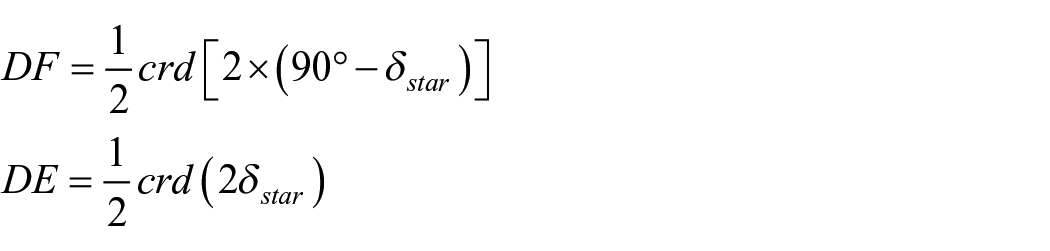
First, assuming the radius OD of the circle to have the same value R of the TOC, the segments DF and OF = DE can be readily calculated applying the TOC (or by interpolating from it) to the triangle ODE (Figure 1, left):

D F = 1 2 c r d [ 2 × ( 90 ° − δ s t a r ) ] D E = 1 2 c r d ( 2 δ s t a r )

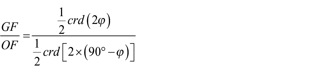
Next, we apply the TOC to triangle OFG (shaded triangle in Figure 1, left). However, this step involves the CRT. In fact, it is very important to note that the triangle OFG can be inscribed in a circle with center O and radius OG, which is smaller than the radius R used for the TOC: thus, the TOC entries corresponding to angles φ and 90°− φ cannot be directly used. This is due to the nature of the TOC itself, which is a table of segments, unlike the modern trigonometric functions, so that the values of these segments depend on the value of the radius of the circle for which the TOC has been calculated. In particular, when the TOC is applied to a right triangle, it is necessary that the hypotenuse be equal to the radius R of the table of chords, like in triangle ODE in Figure 1, left. Otherwise, every time the TOC is applied to a right-angle triangle whose hypotenuse is different from R (such as triangle OFG), a proportion needs to be made between such triangle (of which we must know at least one of the three sides) and a similar one with hypotenuse R.

In the case of triangle OFG, we determined side OF = DE, so that side GF can be determined through such a proportion and the CRT:

G F O F = 1 2 c r d ( 2 φ ) 1 2 c r d [ 2 × ( 90 ° − φ ) ]

This use of proportions and CRT is implicit in all the uses of the TOC we do in this work. The same use of the CRT was made by Edwards (1984). ¹⁸

The third and last step yields directly the angle γ. Applying the CRT to triangle HGF in Figure 1, right, knowing that HF = DF (they are both the radii of the stellar parallel circle), we have:

G F H F = 1 2 c r d ( 2 γ ) R

which allows us to determine the value of the angle γ from the TOC. ¹⁹

As noted earlier, once the angle γ is known, the length of the parallel above the horizon (clockwise from H to K in Figure 1, right) can be readily determined, and the culminating point of the equator α_culm can be readily calculated from the right ascension α_star of the star as

α c u l m = α s t a r + H F ^ D = α s t a r + { 90 ° + γ w i t h δ s t a r > 0 90 ° − γ w i t h δ s t a r < 0

It is important to note that this procedure is mathematically identical to the analemma procedure itself. In fact, Figure 2 displays a 2D rendering of the analemma geometry necessary to solve Problem A for a star in the northern hemisphere. Figure 2 can be interpreted as the combination of the two figures in the top row of Figure 1. The circle NLDSB and the lines it includes are identical to Figure 1, top left: the celestial sphere is seen from the west direction, the plane of the celestial equator and of its parallels are shown as straight lines and the south meridian is the circle NLDSB centered in O, while the Earth’s rotation axis is inclined relative to the local horizon by the local latitude φ and the parallel with declination δ_star,where the star in question orbits, is shown by the segment BD, the star sets (and rises) in point G and culminates in point D; point F is the intersection between the parallel plane where the star is and the Earth’s axis. The half circle BHQD, which is identical to Figure 1, top right, represents the 90° projection of the parallel BD into the plane of the south meridian: point Q is the projection of point F, and point H is the projection of point G and represents the position of the star on the parallel at the time of setting (or rising). Point E is the projection of point D onto the plane of the celestial equator. The same steps can be equally applied to the geometries in Figures 1 and 2, so that the difference between these two approaches is only given by a different way of visualizing the problem: while Figure 1 can be imagined as derived from looking at a celestial globe from two different points of view, Figure 2 involves a transformation of a 3D geometry into a 2D settings and is thus conceptually more advanced. When such a projection was introduced in ancient Greek geometry, we do not know; still it represented an advance in that it allowed one to approach 3D spherical problems using a single, more compact 2D plane geometry setting.

OPEN IN VIEWER

Figure 2.

Geometry related to Problem 1 for a setting star with positive declination as seen with an analemma construction. The celestial sphere centered on O is seen from the West direction, with the circle NLDSB being the south meridian. The star (having a declination δ_star and setting at point G), rotates around the Earth’s axis along the parallel BD (seen as segment BD); the curve BHQD represents the projection of the parallel BD on the plane of the south meridian, and the point H represents the position of the star in the projected parallel. Point E marks the distance from the parallel’s culmination point D to the equatorial plane.

Problem B: Calculate the culminating point of the ecliptic

According to Sidoli, this is the primary problem ²⁰ of Hipparchus’ dia tōn grammōn method, but in reality it consists of a simple change of coordinates between the Equatorial System and the Ecliptic System for a point lying on the celestial equator only applied to the ecliptic longitude (i.e. the ecliptic and equatorial latitudes are of no interest). Sidoli applies Menelaus’ Theorem for the first time to solve it, ²¹ but it is possible to reach the solution by means of the TOC, the CRT, and EI47, once the obliquity ε is known. In general, the procedure we describe below can be applied to a similar layout involving any pair of great circles of the same sphere, and allows us to determine the position, relative to the intersection of these two circles, of a pair of points connected by a third great circle perpendicular to one of them: this property is critically important to solve Problem C.

Finding the ecliptic longitude of point C of the ecliptic sitting on the same equatorial meridian of point B on the celestial equator means solving a problem set as shown in Figure 3, where A is the Spring Equinox. The geometry of this problem is the same for both equinoxes, and for right ascension angles (RA) preceding or following the Equinox itself.

OPEN IN VIEWER

Figure 3.

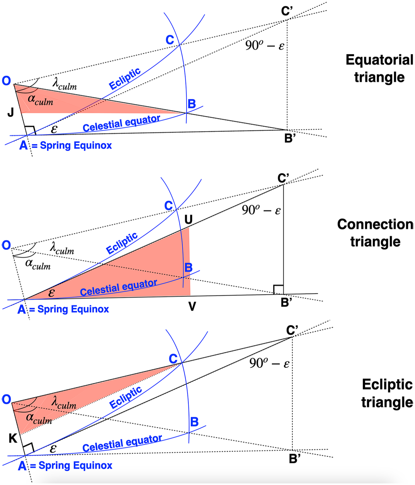
Change of coordinates close to the Spring Equinox (A). α_culm: culminating right ascension; λ_culm: culminating ecliptic longitude; ε: obliquity of the ecliptic. AB is the arc of the celestial equator corresponding to angle α_culm; AC is the arc of the ecliptic corresponding to angle λ_culm. The arc BC belongs to the south meridian. Top: working on the equatorial triangle OAB′, shaded triangle OJB is similar to OAB′. Middle: working on connection triangle AB′C′, shaded triangle AVU is similar to AB′C′. Bottom: working on the ecliptic triangle OAC′, shaded triangle OKC is similar to OAC′.

Figure 3 shows a 3D rendering of the problem. All three panels (top, middle, bottom) show the same section of the celestial sphere, centered in O with radius OA = OB = OC = R. The circular sector OAB lies on the equatorial plane, so that the arc AB is the section of the celestial equator corresponding to the culminating right ascension α_culm calculated in Problem A. In the same way, the circular sector OAC lies on the ecliptic plane, so that the arc AC is the section of the ecliptic corresponding to the culminating ecliptic longitude λ_culm; the arc BC belongs to an equatorial meridian (in this case, the south meridian). The segments AC′ and AB′ are tangent to the ecliptic and the celestial equator, respectively, and are delimited in C′ and B′ by the extensions of radii OC and OB, respectively; the segment B′C′ is perpendicular to AB′.

From Problem A, we have calculated the culminating right ascension α_culm corresponding to the setting of a star, so α_culm is the right ascension of point B. The problem consists of determining the corresponding culminating ecliptic longitude λ_culm as the point of the ecliptic sitting on the culminating meridian. The problem can be solved considering in series three triangles in Figure 3: the equatorial triangle OAB′ (top), the connection triangle AB′C′ (middle), and the ecliptic triangle OAC′ (bottom). We use the same TOC used in Problem A, applying it to a sphere with the same radius R as the TOC; to this end, in each of the panels we also show right triangles (shaded) whose hypotenuse is equal to R, which will be necessary to apply the TOC to Problem B.

We start from the equatorial triangle (Figure 3, top). We need to find side AB′: the right triangle OAB′ has an (unknown) hypotenuse larger than R so that the TOC cannot be directly applied to it: to this end, we draw a similar (shaded) triangle OJB, whose hypotenuse OB = R, and determine AB′ through a simple proportion between similar triangles OAB′ and OJB and the CRT:

A B ′ O A = J B O J

knowing both sides JB and OJ from the TOC:

J B = 1 2 c r d ( 2 α c u l m )

O J = 1 2 c r d [ 2 × ( 90 ° − α c u l m ) ]

We now move to the connection triangle AB′C′ (Figure 3, middle), with the goal of determining side AC′. Again, this is a right triangle with hypotenuse larger than R, so we draw a similar (shaded) triangle AVU, with UV parallel to B′C′ and hypotenuse UA = R. Knowing AB′ from the equatorial triangle, and using a simple proportion:

A C ′ A B ′ = U A A V

we can apply the CRT to determine AC′ knowing AB′ from the equatorial triangle and AV from the TOC ²² :

A V = 1 2 c r d [ 2 × ( 90 ° − ε ) ]

Knowing AC′ allows us to move into the ecliptic triangle OAC′ (Figure 3, bottom) where we draw a new right (shaded) triangle OKC, with KC parallel to AC′ and hypotenuse OC = R: to determine the side KC we resort to the same method as with the previous two triangles, using a proportion and the TOC:

A C ′ O C ′ = K C O C

This time however we have two unknowns: KC and OC′. The latter can be determined using EI47:

( O C ′ ) 2 = ( O A ) 2 + ( A C ′ ) 2

Once we solve for KC, the angle λ_culm can be determined directly from the TOC through

1 2 c r d ( 2 λ c u l m ) = K C

It is important to note that this geometrical setup also allows the user to walk the opposite route: knowing the angle λ_culm, one can determine α_culm. Again, the solution to Problem B developed here applies to any other pair of great circles intersected by a third one perpendicular to one of them; this property is critically important to solve the Problem C.

Problem C: Calculate the rising point of the ecliptic

Once the culminating point of the ecliptic λ_culm is determined, we are left with the last step of Hipparchus’ method, which yields the rising point of the ecliptic. Since the ecliptic is a great circle, this method can actually provide both the rising and setting point of the ecliptic for a given value of λ_culm, since they will be simply separated by 180°. This is where Menelaus’ Theorem, again invoked by Sidoli as the solution, ²³ is most useful: in fact, solving this problem using the simpler geometrical tools as we do in this paper involves two steps, each requiring a long series of calculations. Figure 4 summarizes the problem: the first step consists of determining the angle E′OS = 90°− θ corresponding to the arc E′S on the horizon between the rising point of the ecliptic E′ and the south direction S; in the second step the angle E′OC = Δλ corresponding to the arc E′C on the ecliptic from rising to culmination is determined through a change of coordinates from the horizontal to the ecliptic system, using the same method as in Problem B but considering that the inclination ε′ of the ecliptic axis relative to the local vertical changes during the day due to the Earth’s own rotation. Once Δλ is known, the ecliptic longitude of the rising point is given by

λ r i s e = λ c u l m + Δ λ

In order to determine Δλ, it is necessary to determine both θ and ε′.

OPEN IN VIEWER

Figure 4.

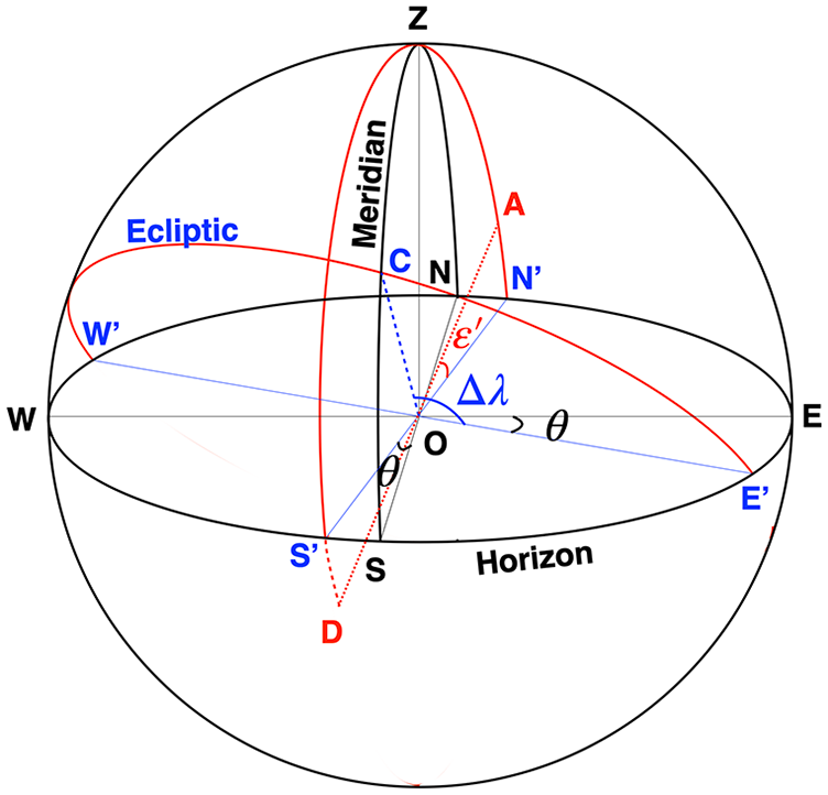
Image of the celestial sphere. The circle NWSE is the horizon, while SZN is the south meridian. The ecliptic circle E′CW′ intersects the horizon plane along the E′W′ line, inclined relative to the east-west direction EW by an angle θ, and culminates in point C, whose ecliptic longitude is λ_culm. The ecliptic axis AD intersects the celestial sphere in points A (north ecliptic pole) and D (south ecliptic pole) and is inclined by an angle ε′—the local obliquity. The angle Δλ separates the culminating point of the ecliptic C from the rising point E′.

Sidoli considered this third step as a secondary problem, but in reality it is the most geometrically complex and computationally expensive, making its application rather cumbersome. In fact, while Menelaus’ Theorem as applied by Sidoli allows for the solution in one simple, neat calculation, in the following geometrical method two steps are necessary, each involving multiple calculations. Still, despite the complexity, this problem can again be solved through the use of only the TOC and the CRT.

First step

To solve this problem, it is useful to refer to Figure 5, which shows the celestial sphere centered in O as seen from the zenith (Figure 5, left) and the west (Figure 5, right) direction. In the left panel, the circle ESWN is the local horizon, point Z is the local zenith, and the SN line is the south meridian. The ecliptic is represented by the nearly circular ellipse AE′CDW′ culminating in C and intersecting the horizon in the two points E′ and W′ separated by 180°; the horizon’s diameter N′S′ is perpendicular to segment E′W′, both lying in the plane of the horizon. θ is the angle between diameters N′S′ and NS which we seek to determine. The circle centered in O′ (shown as a smaller ellipse due to the projection onto the horizontal plane) represents the daily circle made by the ecliptic pole on the celestial sphere around the Earth’s rotation axis (where the O′O segment lies); point A represents the position of the ecliptic pole in this circle at the time of υ Boo’s setting and is indicated by the angle β, which we assume to be zero when the summer solstice culminates (corresponding to RA = 6 h00 m, λ = 90°): since β changes at constant speed following the Earth’s own rotation, covering 360° in 24 hours, the angle β is the same as the RA of the setting ecliptic point shifted by 6 h, or 90°:

β = α c u l m − 90 °

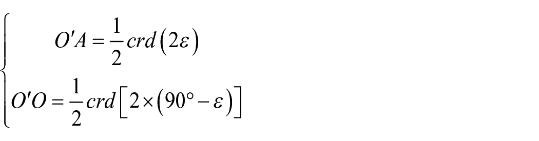
In this layout, it is first important to note that there are a few fixed segments involved in the procedure that can be calculated once and for all and applied to the rising or setting of any star. These are the radius O′A of the circle made by the rotation of the ecliptic pole, the distance O′O between the center of that circle to the center O of the celestial sphere, and the projection O″O of the O′O segment on the local vertical direction. Using a TOC based on the radius R of the celestial sphere, these segments can be determined from the shaded square triangles in Figure 5. Considering the shaded triangle OO′A in the left panel, we note that this is a square triangle whose hypotenuse is equal to the radius R of the sphere, so that the TOC readily provides its sides:

{ O ′ A = 1 2 c r d ( 2 ε ) O ′ O = 1 2 c r d [ 2 × ( 90 ° − ε ) ]

OPEN IN VIEWER

Figure 5.

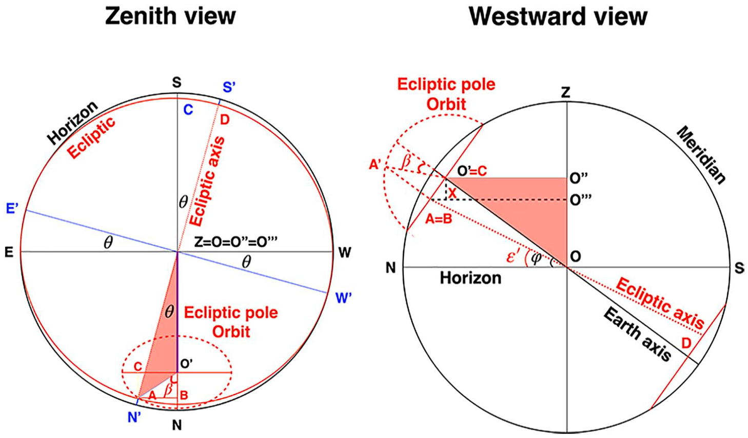
Left: celestial sphere as seen from the Zenith point Z. The ecliptic north pole A rotates around the earth axis (projected along the SON direction) making the circle centered in O′, and its position is indicated by angle β relative to the O′B direction. The thick O′O line indicates the shaded triangle O′O′′O in the right panel as seen from the Zenith point. Right: Celestial sphere as seen from the west. O′O is the direction of the Earth’s axis, while the circles of the orbit of ecliptic north pole A and south pole D are collapsed into the thick lines perpendicular to the Earth’s axis. The dotted analemma provides a visual illustration of the orbit of point A (not used in the text). Point X marks the distance from center O′ to line O′′′B.

On the other hand, the segment O′O is the hypotenuse of the shaded square triangle O″O′O in Figure 5, right, and is shorter than R, so that the TOC needs to be combined with a proportion and the CRT to yield O″O:

O ″ O O ′ O = 1 2 c r d ( 2 φ ) R

The solution passes through the determination of the segment O′′′O, which can be determined from the two shaded right triangles in Figure 6. Considering triangle O′BA on the left, the TOC and the CRT can be applied again to determine the segment O′B as

O ′ B O ′ A = 1 2 c r d [ 2 × ( 90 ° − β ) ] R

OPEN IN VIEWER

Figure 6.

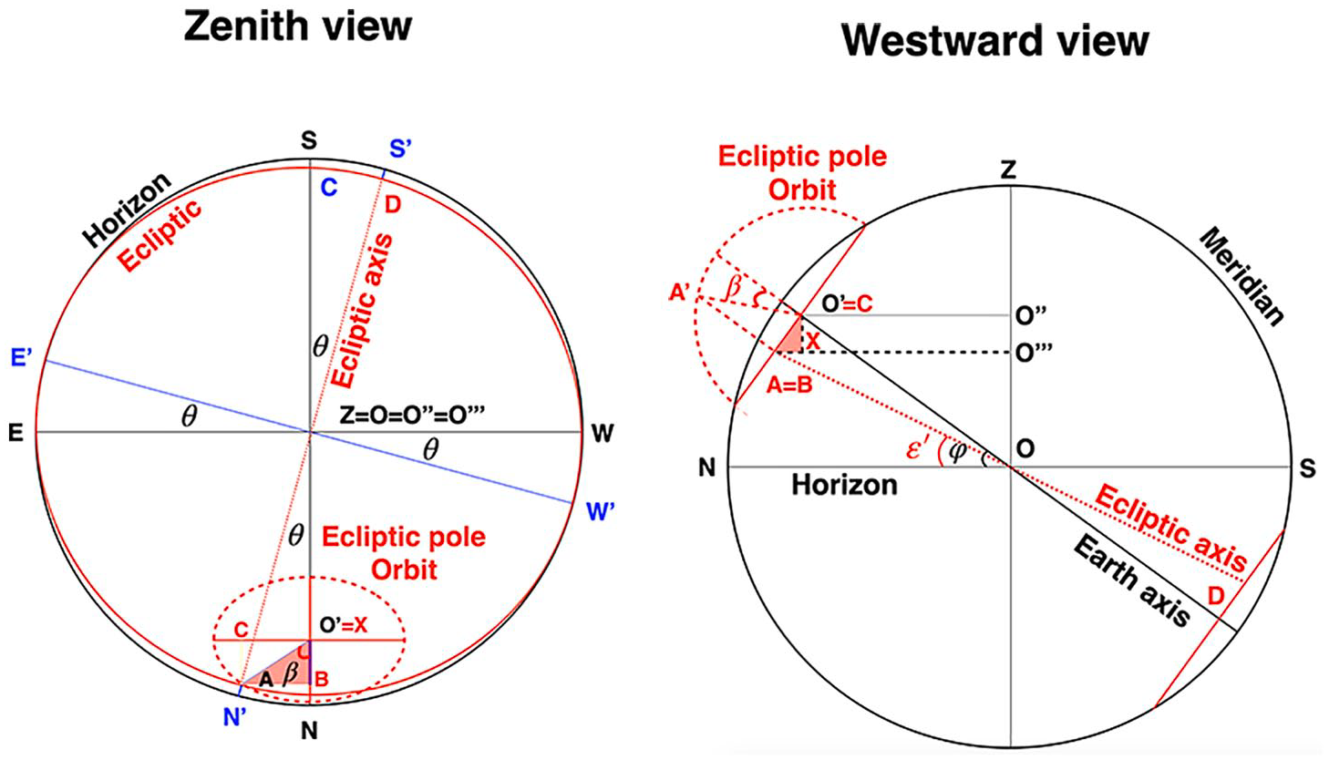
Same as Figure 5, with shaded triangle O′XB in the right panel; the same triangle is shown as thick line O′B in left panel.

Segment O′B in turn serves as hypotenuse for shaded right triangle O′XB in the right panel, which allows, through the usual combination of TOC and CRT, the determination of the side O′X:

O ′ X O ′ B = 1 2 c r d [ 2 × ( 90 ° − φ ) ] R

Since O″O′′′ = O′X, we can find O′′′O as

O ‴ O = O ″ O − O ′ X

Knowing O′′′O allows us to move to Figure 7 and work on two new shaded right triangles. Considering triangle O′′′OA in the right panel (whose hypotenuse OA is the radius R of the sphere) the local obliquity ε′ can be readily determined from its chord in the TOC:

O ‴ O = 1 2 c r d ( 2 ε ′ )

OPEN IN VIEWER

Figure 7.

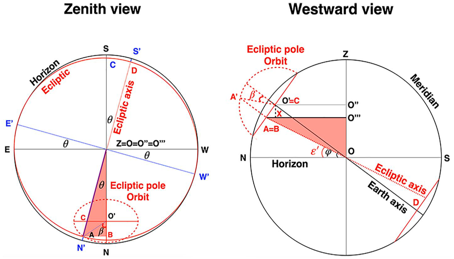
Same as Figure 5, with shaded triangle O′′′AB in the left panel; the same triangle is shown as thick line O′′′A in the right panel, and shaded triangle O′′′OA in the right panel; the same triangle is shown as thick line O′′′A in the left panel.

Which in turn allows the determination of the segment O′′′A as

O ‴ A = 1 2 c r d [ 2 × ( 90 ° − ε ′ ) ]

Working on the shaded right triangle in the left panel, which is parallel to the horizontal plane and has hypotenuse O′′′A shorter than R, we can again combine the TOC and the CRT to determine the angle θ through the determination of its chord:

A B O ‴ A = 1 2 c r d ( 2 θ ) R

Second step

This step is needed to determine E′C, for which it is convenient to refer to Figure 8. This figure shows that the configuration between E′C and E′S (Figure 8, left, taken from Figure 4) is the same as the configuration between AC and AB shown in Figure 3 (replicated in Figure 8, right, for ease of comparison) when we changed the coordinate system from equatorial to ecliptic, with two main differences:

A. The equatorial system is now replaced by the horizontal system; and

B. The inclination of the ecliptic over the horizontal plane, B′Ê′C′ = ε′, depends on time and is different from the value of ε, except when the equinoxes culminate.

OPEN IN VIEWER

Figure 8.

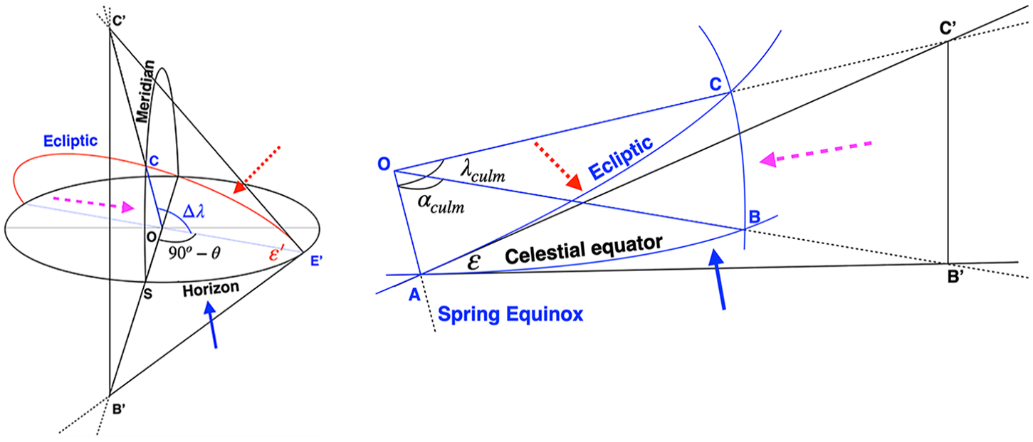
Right panel: same geometry as Figure 3, for a change of coordinates from equatorial to ecliptic coordinate system. Left panel: change of coordinates from horizontal to ecliptic coordinate system. Arrows with the same line type indicate great circles serving the same purpose in both panels. Point E′ is equivalent to Spring equinox A, point S is equivalent to point B, ε′ is equivalent to ε, Δλ is equivalent to λ_culm, and 90°−θ is equivalent to α_culm.

This change of coordinates is made possible by the fact that both the ecliptic and the horizon are great circles, and that the meridian intersects the horizon perpendicularly. Thus, we can repeat the procedure of Problem B to derive the arc E′C (length of the ecliptic from rising to culmination) from the arc E′S (length of the horizon from the rising point of the ecliptic to the southern meridian). The result can be added to λ_culm to obtain λ_rise. Since both the ecliptic and the horizon are great circles, the setting ecliptic point λ_set can be determined by simply subtracting 180° to λ_rise.

It is important to notice that the method we have outlined to solve Problem C can be equally used to determine λ_set first in place of λ_rise by determining the arc W′S. However, it needs to be applied to the calculation of the arc between E′S and W′S, which is smaller than 90°, so that the geometry of the change of coordinates described in Problem B can be applied.

Conclusions

The method we described to solve the problem mentioned by Hipparchus in his Exegesis 2.2.24–2.2.27 has one main strength and one main weakness. The strength is that it is conceptually very simple while still being mathematically exact, and only requires computational tools unquestionably available to Hipparchus: the TOC, the CRT, and EI47. The geometry necessary to unfold all the steps of the solution is rather complex and needs the ability of visualizing a 3D spherical geometry through a series of square triangles in different planes, but it is not unreasonable to imagine that brilliant mathematicians such as the ancient Greeks possessed such visualization skills. The main weakness of this method is that it is computationally very cumbersome and requires a long series of calculations to yield the final results. Even speculating (with no proof) that this is indeed Hipparchus’ own solution, it is highly unlikely that he ever applied it to calculate the vast amount of simultaneous rising and setting data he provided in his Exegesis, making it all the more likely that he simply relied on a globe to determine those data.

However, we would like to stress that the procedure we just described is by no means to be understood as the method that Hipparchus himself was referring to. There is no evidence for it, especially because the treatise he wrote on the subject has been lost. All we wanted to stress is that there is no need of Menelaus’ Theorem, stereographic projections and even the analemma to solve this problem, and that more basic computational tools, certainly at Hipparchus’ disposal, can equally lead to the answer, even though through a much more computationally expensive procedure. It is very well possible that the present solution to this problem could be simplified by the use of geometrical theorems available to Hipparchus, which either we did not consider or for which we do not know the existence: our goal was to show that all the steps in the problem (analemma-like geometries, change of coordinates to and from a spherical system and another, and even the rotation of the sky) could be successfully addressed with very basic geometrical tools unquestionably available to Hipparchus.