Configural Behavior Settings of Crime Event Locations

Abstract

Objectives:

The utility of configural behavior settings is explored as an alternative unit of analysis for place-based criminological research. Four research questions are addressed: (1) How do robberies cluster within certain behavior settings? (2) How are conclusions about robbery’s behavior settings influenced by the distance interval used to measure the proximate environment? (3) Are dominant behavior settings homogeneous across patrol districts? and (4) Is there temporal variability among dominant behavior settings?

Method:

Conjunctive analysis of case configurations is used to construct configural behavior settings around 453 robbery locations in Henderson, Nevada, between 2007 and 2009.

Results:

The major findings of this study are that (1) the majority of personal robberies occur within a small number of dominant configural behavior settings and (2) the composition of behavior settings and the proportion of incidents for which they account varies by the distance interval used to measure the proximate environment, patrol district, and time of day.

Conclusions:

Configural behavior settings provide an alternative unit of analysis that can be used in future place-based research to improve our understanding of criminogenic microenvironments. Replication of this study in other cities that vary in urban design would further demonstrate the merits of this approach.

Keywords

routine activity theory criminological theory rational choice theory measurement crime

And crawling on the planet’s face, some insects called the human race. Lost in time, and lost in space … and meaning.

—“The Criminologist” in The Rocky Horror Picture Show

Introduction

Environmental criminology represents a collection of theoretical propositions that focus on opportunity for offending and the interaction between individuals and the environment (Brantingham and Brantingham 1984, 1991, 2008). Effects of physical settings within the environment and their relationship to crime patterns are of particular interest. Under crime pattern theory (see Brantingham and Brantingham 2008), for example, these physical settings include daily activity nodes, the pathways connecting them, edges along these pathways, and the environmental backcloth that defines this overall space. When crime patterns can be identified and associated with particular aspects of the physical environment, intervention and reduction strategies can be developed and implemented in a more efficient and effective manner.

Over the past several years, studies of physical settings and their effects on crime patterns have focused attention on “places” within which crimes occur. Generally, these studies begin by conceptualizing microenvironments as small areal units that represent neighborhoods or in terms of face blocks¹/street segments (Caplan, Kennedy, and Miller 2011; Eck and Weisburd 1995; Perkins et al. 1990; Taylor 1997; Weisburd, Bernasco, and Bruinsma 2009; Weisburd, Groff, and Yang 2012). Next, individual crime events are assigned to the particular unit of analysis and the expected relationships between characteristics of the physical settings and crime locations are estimated in a statistical model that often assumes that the effects of any particular variable is constant across these microenvironments. Finally, factors associated with criminogenic places where crime clusters disproportionately in space and time are then empirically identified.

When this methodology is adopted, units of analysis that define microenvironments serve as approximations for unique behavior settings that influence human activity (Barker 1968). Consequently, crime events that are assigned to the same unit of analysis are assumed to be influenced by the same physical backcloth. For example, when street segments are used as proxies for behavior settings, it is assumed that the opportunity structure for a crime event at one end of a segment is identical to the structure at every other place along the same street. Because the unit of analysis is predefined in terms of which risk factors are found along/within it, the physical setting associated with a crime event—regardless of where it occurs—is held constant for that “place”. It is more likely, however, that there are subtle but measurable differences between locations within these behavior settings. Therefore, our understanding of criminogenic factors found within the microenvironments of crime is limited when we allow place-based units of analysis to define the space within which incidents occur.

Using data from personal robberies² that were recorded in Henderson, Nevada, as a case study, the current investigation applies an alternative approach to studying criminogenic behavior settings. Building on the original conceptualization described in the ecological psychology literature (Barker 1968), behavior settings are defined in the current investigation as unique combinations of activity nodes, time periods, and land-use areas that define crime event locations, which are created through conjunctive analysis of case configurations (CACC; Miethe, Hart, and Regoeczi 2008). Results of this study and its comparative methods are discussed in terms of their implications for future place-based criminological research.

Review of the Relevant Literature

In an attempt to better understand crime patterns and to develop scientifically based intervention and prevention strategies, place-based criminology shifts attention from persons to places. Much of this work seeks to strike a balance between identifying a unit of analysis that is large enough to represent unique approximations of Barker’s (1968) behavior settings, but not too large to lose important information about within-group variations in both levels of crime and in those characteristics of the microenvironment believed to influence it.

Crime Hot Spots and Place-based Research

Scholars have long been interested in better understanding the nonrandom, spatial concentrations of crime in places. For example, the early 20th-century Chicago ecologists identified “natural areas” for crime within the city’s “zone in transition” and this concentration of particular crime in particular geographical areas of cities continues to be well documented (Sampson and Groves 1989; Shaw and McKay 1942). As a more direct measure of crime’s clustering in “hot spots,” Sherman and colleagues (1989) discovered that during a single year in Minneapolis 50% of all calls for service were generated from 3% of all local addresses. This high concentration of criminal incidents in a relatively small set of locations has also been widely replicated (Eck, Clarke, and Guerette 2007; Weisburd et al. 2012).

Using various point pattern techniques, including modal hot spot analysis, spatial and temporal analysis of crime (STAC; Spring and Block 1989), nearest neighbor hierarchical clustering (Hartigan 1975; Ward 1963), and K-means clustering (Ball and Hall 1970; Thompson 1956), early place-based research used crime hot spots as a unit of analysis. However, results produced from point pattern methods define spatial clusters of incidents in terms of geometric areas such as spatial ellipses or convex hulls that can be relatively large in area. As a result, few of today’s place-based scholars study crime hot spots created from these techniques.

Crime hot spots can also be created by aggregating discrete event locations to areal units such as grids, census boundaries, or other administrative areas (e.g., patrol districts or police beats) and then testing the spatial association between them. Studies of places that have been identified as crime hot spots through aggregation methods are more common in the existing empirical literature. For example, Sorg and colleagues (2013) recently analyzed the spatial association between crimes aggregated to police beats within Philadelphia in order to explore the longitudinal deterrent effects of foot patrols. Like hot spots created by point pattern analysis, however, depending on the size of the areal units that are employed, the utility of aggregation methods may be limited in place-based studies.

Chainey, Tompson, and Uhlig (2008), as well as Hart and Zandbergen (2014), suggest that kernel density estimation (KDE) offers a useful alternative for studying crime and place. KDE involves estimating the density of crime across an entire two-dimensional study area, based on the known locations of discrete events (Bailey and Gatrell 1995). Since KDE allows users to define the search radius and grid cell size used to detect and display hot spot results, the size of microenvironments can be determined a priori. For example, in risk terrain modeling (RTM), KDE is used to not only identify places where crime clusters but also where the spatial influence of factors associated with crime is also more or less likely to be located (Caplan and Kennedy 2010; Kennedy, Caplan, and Piza 2011). When the microenvironment is defined by the user as a single block or two, recent evaluations of RTM suggests that it offers an accurate way of identifying patterns of elevated crime risk across an entire landscape (Caplan, Kennedy, and Baughman 2012; Edmonds and Mallard 2011; Yerxa 2013). However, since KDE relies on several user-defined parameter settings, there may be considerable variation in what could be classified as a criminogenic place. For many place-based scholars, this is problematic, as they desire a more stable unit of analysis. In response, an increasing number of place-based studies have turned to units of analysis that approximate “behavior settings.”

Behavior Settings and Human-environment Interaction

Behavior settings as a unit of analysis emerged from the ecological psychology literature nearly six decades ago (Barker 1968; Barker and Wright 1955). According to Barker (1968), a behavior setting has both structural and dynamic elements and is defined by six attributes. First, a behavior setting consists of at least one standing pattern of human behavior that is influenced by the environment. That is, regardless of who is in a behavior setting similar patterns of human-environment interaction will be observed. Second, human-environment interaction within a behavior setting consists of both man-made and naturally occurring elements (i.e., the milieu or soma). Third, the milieu must encompass a behavior setting; that is, according to Barker, a particular behavior setting will be entirely enveloped by the milieu. In this case, one can envision a store (milieu) encompassing the behavior of those within it, during its normal operating hours. In other words, the store is circumjacent to the behavior. Fourth, the milieu is similar in structure to the behavior it envelopes. Barker uses a church service to illustrate this point. He explains, “ … both the pews (milieu) and the listening congregation (behavior) face the pulpit (milieu) and the preaching pastor (behavior)” (p. 19). Fifth, collectively, the behavior-milieu parts are called synomorphs. According to Barker, the structure of a behavior setting is defined by a set of synomorphs. Finally, the synomorphs that make up the structural attributes of a behavior setting have a specified degree of interdependence. In other words, they are unique but they are also interrelated.

Studying human-environment interaction within a small Midwest town in Kansas, Barker (1968) quantified 220 unique behavior settings based on these criteria. Behavior setting genotypes that he identified included a bank (n = 1), bus stops (n = 2), fire stations (n = 2), grocery stores (n = 3), hotels (n = 3), a parking lot (n = 1), parks and playgrounds (n = 4), and a welfare office (n = 1). Within the context of environmental criminology, many of the behavior settings that Barker discusses are analogous to activity nodes located within an environmental backcloth (see, e.g., Brantingham and Brantingham 2008:87-89). They are ecological units of analysis that represent more than the physical or social environment. Rather, they are places that define specific types of human-environment interaction (for similar arguments, see Brantingham and Brantingham 2008; see also Felson 2006).

The connection between behavior settings and activity nodes is important to criminological research because existing contemporary scholarship has identified particular activity nodes in the proximate environment and the “awareness space” of the potential offenders and targets that facilitate and/or attract crime (Brantingham and Brantingham 2008). For example, regardless of whether they are considered crime generators or attractors, past research suggests that patterns of criminal activity often cluster in and around certain physical characteristics of behavior settings, including check-cashing outlets and ATMs (Holt and Spencer 2005), pawnshops and bars (Roncek and Maier 1991), schools (Block and Block 1995; Roncek and LoBosco 1983), and public transportation nodes (Hart and Miethe 2014; Levine and Wachs 1985; Loukaitou-Sideris 1999; Newton 2004). Although this body of research informs us about characteristics of the physical environment that are associated with crime, the challenge for contemporary place-based scholars is to conceptualize an appropriate approximation of Barker’s (1968) ecological unit of analysis. In other words, what measure of ecological aggregation best represents the sociophysical context that underlies Barker’s behavior settings and related concepts (e.g., activity and awareness space, microenvironments)?

Contemporary Approximations of Behavior Settings

Some scholars argue that “neighborhoods” offer appropriate units of analysis when studying criminogenic places. For example, to learn more about the effects of physical settings on crime, Oberwittle and Wikström (2009) studied more than 6,000 U.K. residents. They aggregated survey responses to different areal units to examine environmental influences on crime and perceptions of neighborhoods. They demonstrated that participants’ attitudes toward social cohesion and informal social control were influenced by environmental factors in the immediate area around where respondents lived. Perceptions of the environment were also more homogenous when the smallest unit of analysis was used to represent neighborhoods. They concluded that smaller units of analysis were theoretically superior to larger units because they better approximated Barker’s (1968) behavior settings. However, for many researchers, areal units—even small ones that represent neighborhoods—are too large to approximate behavior settings because the within-group variation of factors that explain crime is still too large.

When studying crime and place, Taylor (1997) suggested several reasons for why face blocks offered more appropriate approximations of behavior settings than neighborhoods. First, he argued that face blocks contain residential life, they have different characteristics, and that life within them is influenced more by on-block events than off-block events (i.e., events in the overall neighborhood). Second, he contended that the social climate on a face block is better understood by residents than the social climate of their larger neighborhood; but that block life is conditioned by features of adjoining blocks (i.e., blocks immediately behind, next to, or in close proximity of another block). Finally, Taylor suggested that the behavior settings of some blocks may change over time; but for most, they offer stable and enduring spatial units of analysis. Following Taylor’s recommendations, face blocks—also referred to as street segments—are commonly used as a place-based unit of analysis in contemporary research because they are believed to be good approximations of behavior settings.

For example, Weisburd et al. (2012) recently found that over the course of a 15-year period in Seattle, about half of all crime incidents were associated with approximately 5% of all the city’s street segments. Grouping these streets together to define their crime trajectories over time, Groff, Weisburd, and Morris (2009) concluded that there was considerable variation between streets in terms of spatial crime patterns. Even when street segments were in close proximity to or even adjacent to one another, negative spatial autocorrelation was often observed (i.e., streets near one another had different/opposite crime trends). Based on these observations associated with street segments, Groff et al. (2009) argued that this particular unit of analysis could represent behavior settings nested within larger social units such as neighborhoods and therefore offer place-based scholars a suitable unit of analysis.

An Alternative Conceptualization

Collectively, existing literature demonstrates certain consistencies with respect to place-based research. First, it reflects considerable interest in understanding the microenvironment of crime and particularly the physical aspects of the environment that may attract or generate criminal activity. Second, there has been a general trend in place-based criminology to seek units of analysis that are good approximations of Barker’s (1968) behavior setting. Third, there is a lack of consensus with respect to which behavior-setting proxy is most appropriate, but the utility of street segments has been repeatedly demonstrated in more contemporary scholarship. Building on these efforts, this study offers an alternative conceptualization of behavior settings in order to study crime and place.

Using CACC (Miethe et al. 2008), behavior settings are defined in the current investigation as unique combinations of activity nodes, time periods, and land-use areas surrounding the locations of robbery events. This approach allows for the location of a crime event to be identified first and then the physical characteristics of the proximate environment to be constructed around it. This differs from most contemporary approaches to place-based research, whereby the physical characteristics of the unit of analysis are predefined and crime events are associated with them when incident locations are assigned to a particular unit. For example, if street segments are used, the physical characteristics for each segment are known and a crime located along a particular street will have the physical characteristics of that segment assigned to it. The result may be a loss of information about within-segment variability in the opportunity structure for crimes along that street segment. Instead, by allowing the behavior setting to be constructed around an incident—as will be done in the CACC that follows—a richer understanding of criminogenic microenvironments can be realized.

The Current Investigation

Using data from robberies that were recorded in Henderson, Nevada, between 2007 and 2009, we apply CACC to define configural behavior settings in order to answer four research questions:

Research Question 1: To what extent do robberies cluster within certain “places”, when place is defined by configural behavior settings?

Identifying the number of observed behavior settings, dominant behavior settings, and the proportion of all robbery events accounted for by dominant behavior settings provide answers to our first research question.

Research Question 2: When the distance used to define the proximate environment of a robbery varies, are the dominant behavior settings homogeneous or do they vary significantly?

Our second research question is answered by comparing the rank-order correlations of behavior setting profiles across three different conceptualizations of “proximity.” In addition, we examine the extent to which individual elements of dominant behavior settings are more or less likely to be present or absent from these profiles than expected in order to determine the impact that each focal variable has on the overall composition of dominant behavior settings.

Research Question 3: Are the dominant behavior settings of robbery events similar throughout the entire study area or do they vary across space?

We address this question by disaggregating the sample data into three patrol divisions that make up Henderson Police Department’s jurisdiction, comparing the frequency and diversity of dominant behavior settings across all three. We also assess the proportion of incidents accounted for by the dominant profiles within each patrol division.

Research Question 4: Are the dominant behavior settings of robbery events temporally similar or do they vary across time?

Our approach to answering the final research question is similar to the strategy we used to answer our third research question. In this instance, however, data are disaggregated by three patrol shifts (i.e., midnight to 8:00 a.m.; 8:00 a.m. to 4:00 p.m.; and 4:00 p.m. to midnight).

Because existing criminological literature does not offer consistent guidance with respect to distance and the spatial influence of crime attractors/generators, the first two research questions are assessed at three distance intervals (i.e., 500 ft, 1,000 ft, and 1,500 ft), which are approximately equal to one, two, and three blocks in this study area, respectively. Only one distance interval is used to answer research questions 3 and 4 (i.e., 1,000 ft). This interval was chosen based on our findings related to research questions 1 and 2. Collectively, answers to all four research questions enable us to assess the utility of defining criminogenic microenvironments in terms of configural behavior settings.

Data and Methods

Configural behavior settings served as a place-based unit of analysis in this study. Behavior settings were defined by environmental characteristics of known robbery locations, which were constructed through a CACC. Crime incident data (i.e., the location, time, and date of an event), information about activity nodes located within the proximate environment of robberies, and land-use information for legal properties within the study area were used to create each unit of analysis.

Under crime pattern theory (Brantingham and Brantingham 2008), risks associated with particular activity nodes within an urban backcloth are not static and invariant across time and place. Instead, similar combinations of particular activity nodes may vary widely in terms of their classification as risky places or “risky facilities” (Eck et al. 2007), depending on these temporal and spatial dimensions. It is for this reason that measures of both time and space are included in the “hot spot matrix” (Ratcliffe 2004) that derives from our configural analysis of behavior settings.

Crime Incident Data

Crime data were obtained from the Henderson Police Department. Date, time, and location information about known robberies that occurred between January 1, 2007, and December 31, 2009 (n = 453),³ and that were reported to the Federal Bureau of Investigation (FBI) as part of the Uniform Crime Reporting (UCR) Program were used in our investigation. Because this information is official police data, incidents conform to the UCR definition of a robbery.⁴ All robbery locations were successfully georeferenced to the city’s street centerline network, which is an approach that has been shown to produce complete and accurate geocoded crime information (Hart and Zandbergen 2013).⁵

Activity Nodes in the Proximate Environment

Activity nodes in the proximate environment define one characteristic of robbery behavior settings that were examined in the current investigation. This aspect of robbery locations was defined by the presence (1) or absence (0) of eight different activity nodes that previous research suggests may attract/generate crime. Activity nodes used in this study included ATMs, bars/taverns, (public) bus stops, check cashing stores, fast-food restaurants, gas stations, shopping plazas, and smoke shops. Under crime pattern theory, each of these activity nodes may serve to attract and generate robbery incidents because they are indicative of a particular rhythm, ebb, and flow of human activity (i.e., what Felson [2006] refers to as “metabolism”), increase the visibility and accessibility of crime targets at particular times and places, and affect the availability of handlers, guardians, and place managers to decrease criminal motivations and opportunities.

A total of 17 activities nodes where originally considered: adult stores or entertainment sites, ATMs, bars/taverns, (public) bus stops, check cashing centers, fast-food restaurants, gas stations, liquor stores, (public) parking garages, pawnshops, (public) recreation centers, parks, (public or private) schools, shopping malls, shopping plazas, smoke shops, and (public) storage facilities. However, this number was reduced to eight and represents those activity nodes that were frequently observed in robbery environs at the middle (i.e., 1,000 ft) distance band.

Including the remaining nodes that were rarely in the proximate environment of a robbery would significantly increase the number of situational profiles that made up the initial data matrix (i.e., 17 dichotomous variables or 2¹⁷ would yield a data matrix with 131,072 behavioral profiles). More importantly, over 99% of these profiles would be unobserved (i.e., the particular combination of attributes would have a 0 observed frequency in the sample). Consequently, our analysis was based on 8 of the 17 original activity nodes that were considered.

In this study, an activity node was considered “present” in the proximate environment if it was within a predetermined distance of a robbery incident location. Distance intervals of 500 ft, 1,000 ft, and 1,500 ft were used, which are approximately equal to one, two, and three, city blocks in Henderson, respectively. These distance intervals were derived from existing microenvironment criminological scholarship, which suggests that the spatial influence of the physical environment on crime is best defined by a single block/street segment or two (e.g., Caplan 2011; Groff 2011; Weisburd et al. 2009, 2012).

Since Euclidean distance (i.e., straight-line distance) does not consider physical barriers that occur in the natural environment that may restrict movement, this study used “street distance” or service area distance to measure proximity. The use of street distance within this study is also consistent with the notion of the offender’s/victim’s awareness space being “within a visual range of the activity space” (Brantingham and Brantingham 2008:84).

Land-use Data

Zoning and future land-use information was obtained from the City of Henderson’s Community Development Department. A total of 31 different zones are used by the city to classify properties, which we grouped into two general categories, namely, (1) nonresidential/mixed use and (2) residential. Environmental characteristics of all robbery locations are presented in Table 1 by the three distance intervals considered and show that approximately two thirds of the events occurred in nonresidential/mixed-use areas. Descriptions of the temporal (i.e., day and time of a robbery) and spatial (i.e., patrol division) dimension of robberies at each distance are also presented in Table 1.

Table 1.

Characteristics of Robberies’ Proximate Environment, Defined as a Distance of 500 ft, 1,000 ft, and 1,500 ft from the Event Location.

	Distance that Defines Proximate Environment
	500 ft		1,000 ft		1,500 ft
Characteristics	n	%	n	%	n	%
Activity nodes
ATM	164	36.2	236	52.1	275	60.7
Bar/tavern	110	24.3	160	35.3	190	41.9
Bus stop	231	51.0	284	62.7	311	68.7
Check cashing store	64	14.1	110	24.3	148	32.7
Fast-food restaurant	184	40.6	226	49.9	264	58.3
Gas station	133	29.4	193	42.6	216	47.7
Shopping plaza	160	35.3	220	48.6	238	52.5
Smoke shop	87	19.2	138	30.5	170	37.5
Land use
Nonresidential	299	66.0	299	66.0	299	66.0
Residential	154	34.0	154	34.0	154	34.0
Temporality
Day of week
Weekend	131	28.9	131	28.9	131	28.9
Weekday	322	71.1	322	71.1	322	71.1
Time of day
00:00 to 7:59	147	32.5	147	32.5	147	32.5
08:00 to 15:59	104	23.0	104	23.0	104	23.0
16:00 to 23:59	202	44.6	202	44.6	202	44.6

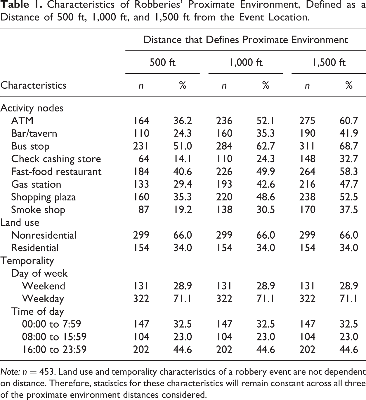
Note: n = 453. Land use and temporality characteristics of a robbery event are not dependent on distance. Therefore, statistics for these characteristics will remain constant across all three of the proximate environment distances considered.

Analytic Plan

CACC was used to answer the four research questions that underlie the current investigation. CACC is similar to qualitative comparative analysis (QCA) methods developed by Ragin (1987, 2013). It offers an alternative approach from more traditional quantitative methods because it explores the relative prevalence of particular combinations of variables (i.e., case configurations) that lead to a particular outcome (e.g., robbery incidents). Unlike traditional approaches, CACC is less interested in main effects (or interactions) of a single predictor or correlations between pairs of variables and instead desires to understand the complex causal relationships created by combinations of all attributes that characterize each focal variable.

CACC can be summarized in three steps.⁶ First, a data matrix or truth table is constructed from focal variables contained in a data file. Each row in the data matrix reflects a unique combination of variable attributes that could be observed in the data. For example, a conjunctive analysis involving three dichotomous variables and two variables with three categories would yield a data matrix with 72 rows (i.e., 3² × 2³ = 72). Columns in this matrix represent each focal variable (e.g., activity nodes, land use, and when a robbery occurred).

Second, each record (e.g., a robbery incident) in the data file is classified into only one of the rows that define the data matrix created and described in step one. Once all cases from the data file are aggregated into the appropriate row of the data matrix, the third step of CACC involves applying decision rules⁷ for defining rare and commonly observed profiles. In this study, these profiles represent the unique configural behavior settings of robberies. After these rules are applied, the resulting data matrix contains one row for each of the dominant behavior settings that are empirically observed in the original data.

Once a CACC data matrix is created, patterns of outcomes (e.g., robberies) among unique profiles (e.g., configural behavior settings) can be analyzed. This study uses various statistical tests to provide answers to the research questions stated earlier, including χ² goodness-of-fit, rank-order correlations (i.e., Spearman’s ρ), and one-sample binomial tests.

Results

Research Question 1

Our initial research question asks, “to what extent do robberies cluster within certain ‘places,’ when place is defined by configural behavior settings?” Results of conjunctive analysis using activity nodes, land-use areas, and days of the week at three distances of spatial influence revealed two distinct patterns, which are conveyed in Figure 1 as a series of cumulative distributions.

Figure 1.

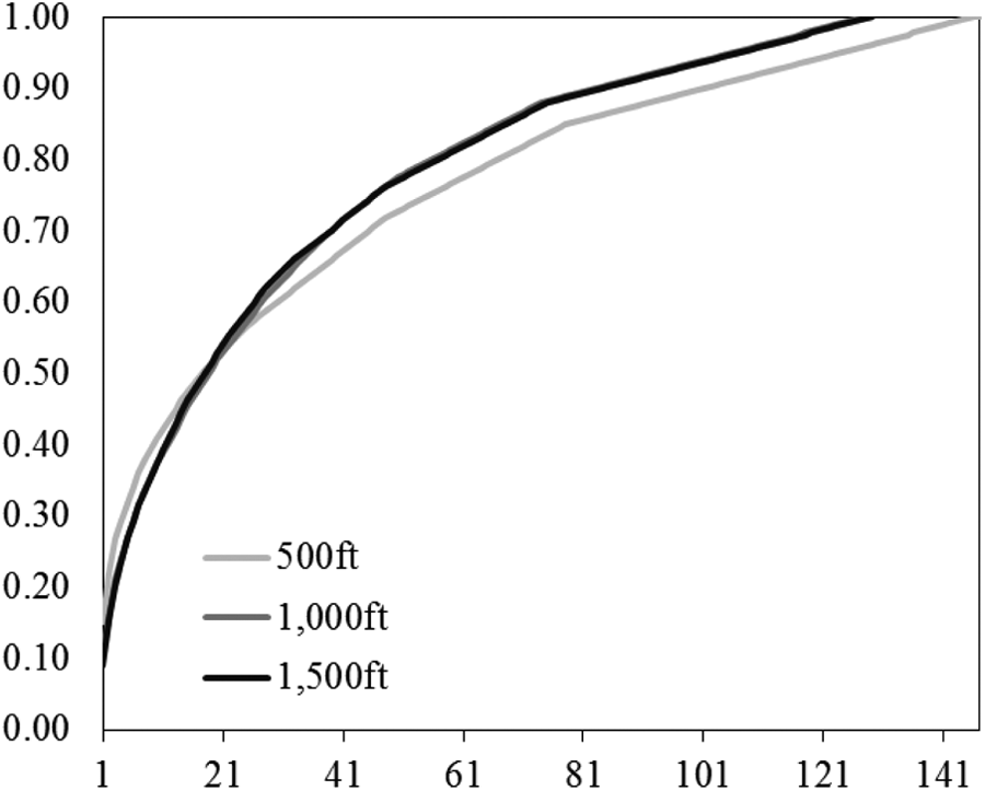
Cumulative distributions for all three conceptualizations of “proximate environment.” The y-axis represents proportion of robberies and the x-axis reflects the number of unique behavior settings. Note that the distribution representing the 1,500-ft distance is nearly identical to and therefore nearly entirely obscures the line representing the 1,000-ft distribution.

First, all robberies included in this study (n = 453) clustered within a small group of unique behavior settings that define an incident’s proximate environment, regardless of which distance was used. When 500 ft was used to define proximity, all incidents clustered within 146 unique behavior settings, compared to 128 for 1,000 ft. The number of unique behavior settings increased to only 129, however, when this distance was increased from 1,000 ft to 1,500 ft.

Second, the proportion of robberies distributed among unique behavior settings was defined by a few dominant profiles, which is evident by the rapid rise in the distribution lines for each distance interval. For example, 18 dominant behavior settings accounted for 51% of all robberies when a distance of 500 ft was used to define the proximate environment. These figures increased to 28 dominant profiles, accounting for 61%, when 1,000 ft was used. The number of dominant profiles and the proportion of robberies for which they account remained relatively unchanged, however, when “proximate” was conceptualized as 1,500 ft (i.e., 28 dominant profiles accounted for 62% of all incidents). Regardless of distance, clustering of incidents among the dominant behavior settings was significantly greater than what was expected (i.e., for 500 ft [χ² = 321.77, df = 17, p < .001]; for 1,000 ft [χ² = 220.55, df = 27, p < .001]; and for 1,500 ft [χ² = 179.06, df = 27, p < .001]).

Collectively, these findings provide answers to our first research question and suggest that the opportunity structure for robbery varies. However, they also indicate that this variation has identifiable patterns and that this patterned variation can be empirically defined in a meaningful way by a relatively small set of distinct places of human-environment interaction. Furthermore, the lack of uniformity of robberies distributed among observed behavior settings suggests that a small percentage of them account for the majority of all incidents in Henderson, which is consistent with contemporary place-based research that suggests a few hot spots account for most crime (Sherman, Gartin, and Buergen 1989; Weisburd et al. 2012) as well as the “risky places” literature that suggests a small subset of places within a larger homogenous group account for most crime (Eck et al. 2007).

Research Question 2

Our second research question asks, “When the distance used to define the proximate environment of a robbery varies, are the dominant behavior settings homogeneous or do they vary significantly?” Table 2 contains the 10 most common configural behavior settings found in the CACC data matrix and their corresponding rank order for each measure of the proximate environment (i.e., 500 ft, 1,000 ft, and 1,500 ft).

Table 2.

Ten Most Common Behavior Settings^a for Robbery Incidents and the Corresponding Rank Order of Profiles When the Proximate Environment Is Defined as 500 ft, 1,000 ft, and 1,500 ft.

Activity Nodes and Whether They Are in the Proximate Environment								Land Use	Day of Week	Rank Order of Profile at a Distance of …
ATM	Bar	Bus Stop	Check Cashing	Fast Food	Gas Station	Shopping Plaza	Smoke Shop			Rank Order of Profile at a Distance of …
ATM	Bar	Bus Stop	Check Cashing	Fast Food	Gas Station	Shopping Plaza	Smoke Shop			500 ft	1,000 ft	1,500 ft
No	No	No	No	No	No	No	No	Residential	Weekday	1	1	1
No	No	No	No	No	No	No	No	Residential	Weekend	2	2	4
No	No	Yes	No	No	No	No	No	Residential	Weekday	3	3	3
No	No	No	No	No	No	No	No	Nonresidential	Weekday	4	13	25.5
No	No	Yes	No	No	No	No	No	Nonresidential	Weekday	5.5	6	9.5
Yes	Yes	Yes	No	Yes	Yes	Yes	Yes	Nonresidential	Weekday	5.5	4	30.5
Yes	No	Yes	No	Yes	No	No	No	Nonresidential	Weekday	7	8.5	9.5
No	No	No	No	Yes	No	No	No	Nonresidential	Weekday	8	—	—
Yes	No	No	No	No	Yes	No	No	Nonresidential	Weekday	9.5	—	—
Yes	No	Yes	No	No	No	No	No	Nonresidential	Weekday	9.5	13	25.5
Total number of observed behavior settings:										146	128	129
Total number of dominant behavior settings:										18	28	28
Percentage of robberies accounted for by dominant behavior settings:										50.6	60.7	62.0

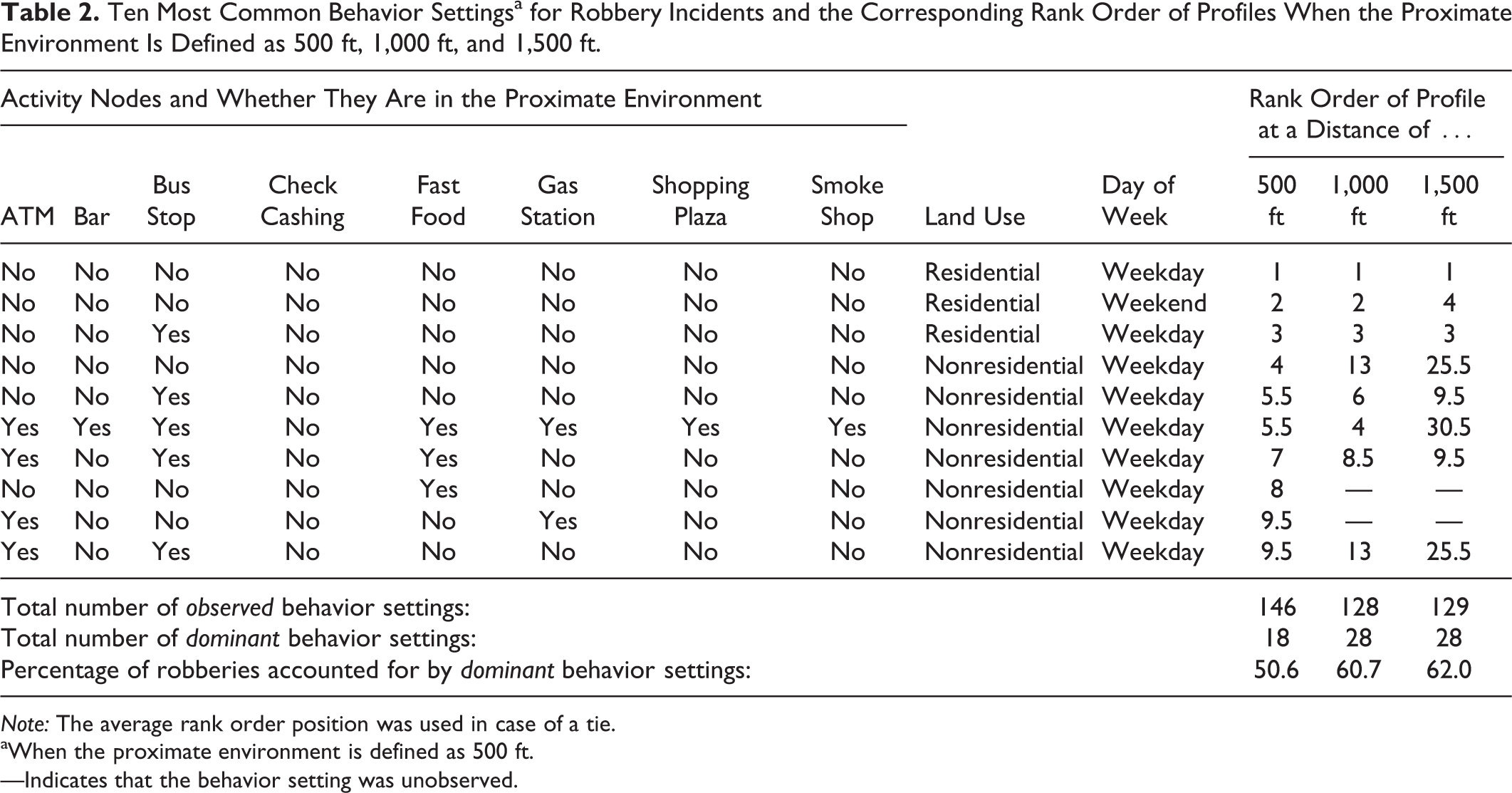
Note: The average rank order position was used in case of a tie.

^aWhen the proximate environment is defined as 500 ft.

—Indicates that the behavior setting was unobserved.

As Table 2 shows, the most common behavior setting observed in this sample was a residential location where all activity nodes were absent from the proximate environment and when the event occurred on a weekday. This profile was the most frequently observed behavior setting regardless of which distance interval was considered.

Although some of the most common behavior settings were consistent across the three distance measures, the overall rank orders of profiles associated with each interval varied in terms of the strength of their correlations. For example, the rank-order correlation between the 500-ft behavior settings and the 1,000-ft behavior settings was only moderately correlated (ρ = .531, p < .001), as was the rank-order correlation between the 500-ft and the 1,500-ft profiles (ρ = .538, p < .001). For distributions of the 1,000-ft and 1,500-ft profiles, however, a much stronger rank-order correlation was observed (ρ = .870, p < .001).

The homogeneity of dominant behavior settings across the three distance intervals was also assessed using a series of one-sample binomial tests, which determined the extent to which individual elements of configural profiles were consistently more or less present or absent than expected. For example, at the smallest distance used to define the proximate environment, only bars (z = 2.12, p = .034) appeared in the dominant behavior setting more often than expected; but smoke shops (z = −3.06, p = .002), incidents that occur in residential areas (z = −2.12, p = .034) and incidents that occur on weekends (z = −3.06, p = .002) were part of the dominant behavior settings less often.

When 1,000 ft was used to define the proximate environment, only bus stops (z = 2.84, p = .005) appeared in dominant profiles more often than expected, while check cashing facilities (z = −2.46, p = .014) and incidents occurring in residential areas (z = −2.84, p = .005) and on weekends (z = −2.08, p = .038) appeared less often.

At the largest distance interval (i.e., 1,500 ft), bus stops (z = 2.84, p = .005) still appeared in the dominant behavior settings more often than expected, while incidents occurring in residential areas (z = −2.84, p = .005) and on the weekend (z = −2.08, p = .038) still appeared less often.

Collectively, these results indicate that distance affects the composition of dominant behavior settings that are associated with robbery locations. Apart from a few of the most common dominant behavior settings that are consistently observed across all three distance intervals, the frequency with which particular profiles are observed varies based on which distance interval is used to define the proximate environment. The greatest heterogeneity among behavior settings is observed when the distance interval increases from 500 ft to 1,000 ft, whereas greater consistency between the rank orders of profiles is observed when the definition of proximity increases from 1,000 ft to 1,500 ft. When viewed in light of results related to our initial research question, current findings indicate that the most robust and stable results of CACC are produced when a 1,000 ft conceptual definition of the proximate environment is used. Therefore, the final two research questions are answered using this distance to define the proximate environment.

Finally, results of the one-sample binomial tests lend support to the idea that in order to better understand criminogenic places we must consider the specific combinations of focal variables that influence the opportunity structure of crime, instead of relying of traditional variable-oriented models that estimate the main effects of individual predictors. In particular, based on the patterns related to the presence/absence of particular elements of configural behavior settings, it appears that the latter approach would have a difficult time accounting for the notion that “context matters.”

Research Question 3

“Are the dominant behavior settings of robbery events similar throughout the entire study area or do they vary across space?” is our third research question. In order to answer it, we disaggregated the original sample into one of the three police patrol divisions (i.e., East, North, and West) and created configural behavior settings for each subarea using CACC. Results are summarized in Table 3 and indicate that robbery behavior settings vary across regions within the broader study area.

Table 3.

Dominant Behavior Settings of Robberies and the Frequency with Which They are Observed in the East, North, and West Patrol Divisions.

ID#	Activity Nodes								Land Use	Day of Week	n	%	Cumulative Percentage
ID#	ATM	Bar	Bus Stop	Check Cashing	Fast Food	Gas Station	Shopping Plaza	Smoke Shop	Land Use	Day of Week	n	%	Cumulative Percentage
Robberies that occurred in the East patrol division (n = 117)
1	No	No	No	No	No	No	No	No	Residential	Weekday	10	8.5	8.5
3	No	No	Yes	No	No	No	No	No	Residential	Weekday	8	6.8	15.4
22	Yes	No	No	Yes	Yes	Yes	Yes	Yes	Nonresidential	Weekend	5	4.3	19.7
23	Yes	No	No	Yes	Yes	Yes	Yes	Yes	Nonresidential	Weekday	5	4.3	23.9
14	Yes	No	Yes	No	No	No	No	No	Nonresidential	Weekday	5	4.3	28.2
25	Yes	No	Yes	No	No	Yes	No	Yes	Residential	Weekday	5	4.3	32.5
Robberies that occurred in the North patrol division (n = 198)
1	No	No	No	No	No	No	No	No	Residential	Weekday	21	10.6	10.6
3	No	No	Yes	No	No	No	No	No	Residential	Weekday	14	7.1	17.7
2	No	No	No	No	No	No	No	No	Residential	Weekend	13	6.6	24.2
4	Yes	Yes	Yes	No	Yes	Yes	Yes	Yes	Nonresidential	Weekday	12	6.1	30.3
7	Yes	No	Yes	No	Yes	No	No	No	Nonresidential	Weekday	7	3.5	33.8
6	No	No	Yes	No	No	No	No	No	Nonresidential	Weekday	6	3.0	36.9
15	Yes	Yes	Yes	No	No	Yes	Yes	No	Nonresidential	Weekday	6	3.0	39.9
20	Yes	Yes	Yes	Yes	Yes	No	Yes	Yes	Nonresidential	Weekday	6	3.0	42.9
21	No	No	Yes	Yes	Yes	Yes	Yes	No	Nonresidential	Weekday	5	2.5	45.5
16	No	Yes	No	No	No	No	No	No	Residential	Weekday	5	2.5	48.0
8	Yes	Yes	Yes	No	Yes	No	Yes	Yes	Nonresidential	Weekend	5	2.5	50.5
19	Yes	Yes	Yes	No	Yes	No	Yes	Yes	Nonresidential	Weekday	5	2.5	53.0
5	Yes	Yes	Yes	Yes	Yes	Yes	Yes	Yes	Nonresidential	Weekday	5	2.5	55.6
Robberies that occurred in the West patrol division (n = 138)
1	No	No	No	No	No	No	No	No	Residential	Weekday	17	12.3	12.3
2	No	No	No	No	No	No	No	No	Residential	Weekend	8	5.8	18.1
5	Yes	Yes	Yes	Yes	Yes	Yes	Yes	Yes	Nonresidential	Weekday	8	5.8	23.9
9	Yes	Yes	Yes	No	Yes	Yes	Yes	No	Nonresidential	Weekend	7	5.1	29.0
17	No	Yes	Yes	No	Yes	Yes	Yes	Yes	Nonresidential	Weekday	6	4.3	33.3
27	Yes	Yes	Yes	No	Yes	Yes	No	No	Nonresidential	Weekday	5	3.6	37.0
10	Yes	Yes	Yes	No	Yes	Yes	Yes	No	Nonresidential	Weekday	5	3.6	40.6

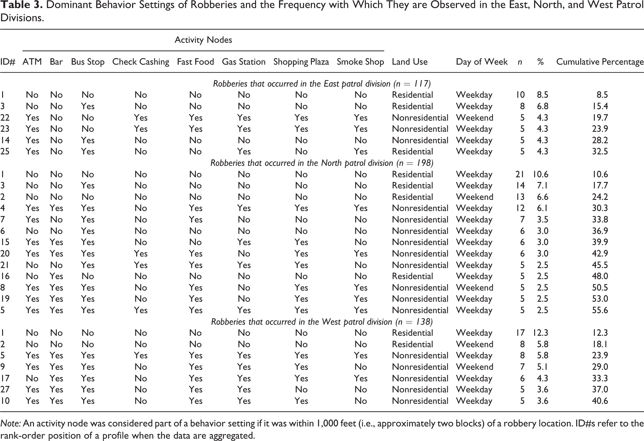
Note: An activity node was considered part of a behavior setting if it was within 1,000 feet (i.e., approximately two blocks) of a robbery location. ID#s refer to the rank-order position of a profile when the data are aggregated.

Dominant behavior settings observed within each of the Henderson Police Department’s three patrol divisions differ in terms of (1) the number behavior setting profiles within each division, (2) the diversity of profiles across divisions, and (3) the amount of robberies accounted for by profiles within each division. For two of the three divisions, incidents within the dominant configural behavior settings also clustered within these profiles significantly.

In the East patrol division (n = 117), robberies were defined by six dominant behavior settings, but the distribution of incidents across these settings was not different than what is expected (χ² = 3.68, df = 5, p = .596). A greater number of dominant behavior settings defined robbery locations in the North patrol division (n = 198). Unlike the pattern observed for the East patrol division, however, the 13 dominant behavior settings in the North exhibited significant nonrandom clustering (χ² = 35.60, df = 12, p < .001) among the dominant profiles. Similar results were observed for the West patrol division (n = 138). Robberies were defined by seven unique combinations of activity nodes, land-use areas, and days of the week; and were clustered among these profiles more than expected (χ² = 13.00, df = 6, p = .043).

Not only did the number/patterns of behavior settings that defined robbery events differ between patrol divisions, but the types of behavior settings found within each area were also unique. For example, the most prevalent behavior setting found when the data were aggregated was still the most prevalent behavior setting identified among the three patrol divisions; however, relatively less common behavior settings were also observed within these subareas. For example, in the East patrol division, the dominant configural behavior settings included case IDs #22, #23, and #25. Similarly, in the North division, behavior settings associated with case IDs #19, #20, and #21 were more commonly observed when the data were disaggregated. In the West patrol division, case IDs #17 and #27 were more common.

The number of robberies that were accounted for by the dominant behavior settings within each patrol division also varied considerably. For example, the dominant behavior settings of robbery in the East division accounted for one third of all incidents. About 56% of all robberies were defined by the dominant configurations found within the North patrol division, whereas the dominant behavior settings accounted for approximately 41% of all robberies in the West patrol division.

For all patrol-specific analysis, these findings suggest that configural behavior settings are qualitatively different across space. Observed variation emerges in terms of both the diversity of dominant behavior settings and the proportion of crime for which they account. These findings indicate that behavior settings constructed through CACC offer a flexible unit of analysis that can be used to define different places across the urban landscape in order to study/address criminogenic microenvironments.

Research Question 4

The fourth and final research question asks whether dominant behavior settings of robbery events varied temporally. In order to answer this question, we considered three time intervals, namely, midnight to 8:00 a.m., 8:00 a.m. to 4:00 p.m., and 4:00 p.m. to midnight. Results presented in Table 4 show moderate variation across each time period when conjunctive analysis was used to define the dominant behavior setting configurations of robbery. In addition, variation within each interval was observed.

Table 4.

Dominant Behavior Settings of Robberies and the Frequency with Which They Are Observed During Patrol Shift 1 (Midnight to 8:00 a.m.), Shift 2 (8:00 a.m. to 4:00 p.m.), and Shift 3 (4:00 p.m. to Midnight).

ID#	Activity Nodes								Land Use	Day of Week	n	%	Cumulative Percentage
ID#	ATM	Bar	Bus Stop	Check Cashing	Fast Food	Gas Station	Shopping Plaza	Smoke Shop	Land Use	Day of Week	n	%	Cumulative Percentage
Robberies that occurred between midnight and 8:00am (n = 147)
1	No	No	No	No	No	No	No	No	Residential	Weekday	14	9.5	9.5
2	No	No	No	No	No	No	No	No	Residential	Weekend	7	4.8	14.3
3	No	No	Yes	No	No	No	No	No	Residential	Weekday	7	4.8	19.0
6	No	No	Yes	No	No	No	No	No	Nonresidential	Weekday	6	4.1	23.1
4	Yes	Yes	Yes	No	Yes	Yes	Yes	Yes	Nonresidential	Weekday	6	4.1	27.2
Robberies that occurred between 8:00am and 4:00pm (n = 104)
1	No	No	No	No	No	No	No	No	Residential	Weekday	11	10.6	10.6
Robberies that occurred between 4:00pm and midnight (n = 202)
1	No	No	No	No	No	No	No	No	Residential	Weekday	23	11.4	11.4
2	No	No	No	No	No	No	No	No	Residential	Weekend	13	6.4	17.8
3	No	No	Yes	No	No	No	No	No	Residential	Weekday	13	6.4	24.3
4	Yes	Yes	Yes	No	Yes	Yes	Yes	Yes	Nonresidential	Weekday	6	3.0	27.2
6	No	No	Yes	No	No	No	No	No	Nonresidential	Weekday	5	2.5	29.7
13	No	No	Yes	No	No	No	No	No	Residential	Weekend	5	2.5	32.2
17	No	Yes	Yes	No	Yes	Yes	Yes	Yes	Nonresidential	Weekday	5	2.5	34.7
5	Yes	Yes	Yes	Yes	Yes	Yes	Yes	Yes	Nonresidential	Weekday	5	2.5	37.1

Note: An activity node was considered part of a behavior setting if it was within 1,000 feet (i.e., approximately two blocks) of a robbery location. ID#s of each behavior setting listed in Table 4 correspond to the behavior setting ID#s presented in Table 3.

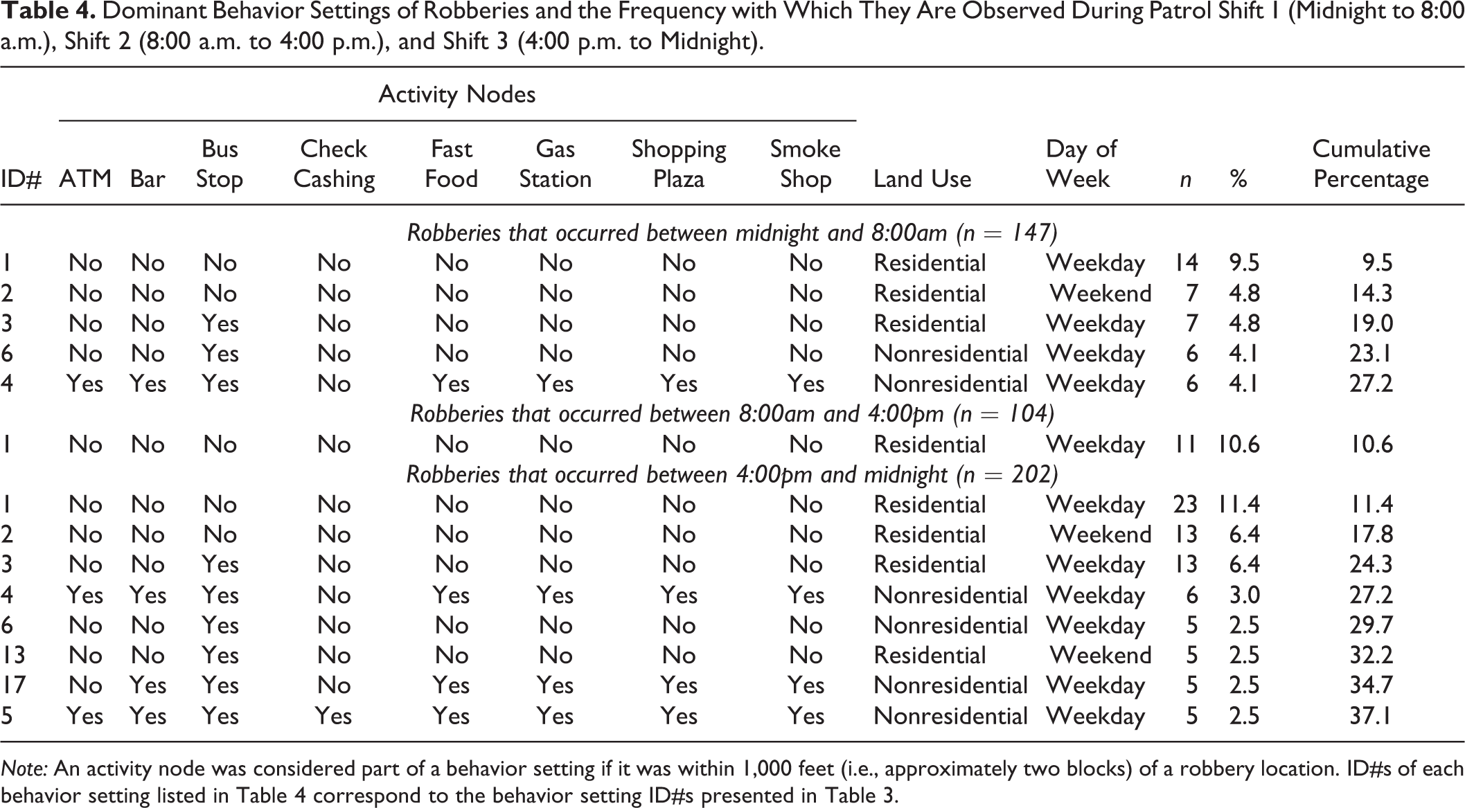
Henderson robberies that occurred between midnight and 8:00 a.m. (n = 147) were defined by five dominant behavior settings, accounting for about one fourth of all incidents. Most of the dominant behavior settings observed during this time period were similar to those found when the data were aggregated; and clustering of incidents among them was similar to what was expected (χ² = 5.75, df = 4, p = .219).

An interesting pattern was observed for robberies that occurred between 8:00 a.m. and 4:00 p.m. (n = 104). During this time period, only one dominant behavior setting emerged, which accounted for about 1 of the every 10 incidents during this time particular time interval. This particular behavior setting is the most prevalent context for robberies in Henderson across all time periods and involves weekday robberies within a residential area that has none of the eight activity nodes within its proximate environment (see Table 4—ID #1 for robberies that occurred between 8:00 a.m. and 4:00 p.m.).

A total of eight dominant behavior-setting configurations were needed to classify all robberies that took place between 4:00 p.m. and midnight (n = 202). The distribution of incidents among these profiles clustered significantly (χ² = 31.99, df = 7, p < .001), accounting for more than a third of all incidents during this time frame.

Similar to the results from our area-specific analysis (see Table 3), the observation of these temporally specific findings further demonstrates the utility of this new unit of analysis for identifying both the dominant and the unique criminogenic microenvironments over place and time

Conclusions

Place-based criminology seeks answers to questions about crime, opportunity structure, and the microenvironment. Although the definition of “place” has evolved over time, the movement of empirical research has generally been toward using a unit of analysis with finer granularity. This movement reflects the contemporary approach because smaller units of analysis improve our ability to detect within-group variation of crime as well as of those factors that are believed to influence it. This study builds on existing place-based literature by investigating whether conceptualizing “place” in terms of configural behavior settings can help further inform our understanding of criminogenic environments.

Answers to this study’s research questions illustrate the utility of configural behavior settings as a new place-based unit of analysis. First, we found that robbery clusters among a relatively small subset of configural behavior settings, that a relatively small percentage of dominant configural behavior settings accounted for the majority of robbery events, and that the diverse causal recipes defining crime can easily be identified using CACC. Second, by disaggregating crime events into three patrol divisions, we demonstrated that configural behavior settings could be used as a unit of analysis to detect and quantify spatial variation in crime. Similarly, we demonstrated how configural behavior settings could be used to quantify temporal variation in crime by disaggregating robberies into three distinct time intervals. Collectively, these findings suggest that in order to better understand criminogenic places, we should consider a unit of analysis that speaks to the specific combinations of factors that influence the opportunity structure of crime events.

Limitations

As with any study, there are certain limitations associated with the current investigation that must be acknowledged. For example, we relied on official data for measures of robbery and land use in order to construct a series of data matrixes that define the proximate environment of robbery locations. Although the limitations of police data are well known, police reports of robberies were the best available data source for this study. Incidents of robbery during criminal transactions (e.g., drug dealing or prostitution) or among known parties (e.g., family or acquaintances) are underreported in official crime data.

Another limitation of this study is its restriction to a particular city within one geographic area in the United States. The actual urban design of this particular suburban area may also impact the nature of observed results. Under these conditions, it is important to replicate the utility of configural behavior settings as a useful place-based unit of analysis in other locations, especially in cities within and outside the United States that have a different urban design and geometry of streets associated with them (see Mehaffy et al. 2010).

Significance and Implications for Future Research

Although the preceding issues limit the generality of our substantive conclusions, this study provides several points of theoretical, practical, and analytical significance for future research. These implications are summarized subsequently.

Theoretically, results of this study are consistent with many of the predictions from environmental criminology and its related theoretical concepts. For example, our findings reinforce the existence of crime’s concentration, using a different measure of spatial-temporal location. It also confirms the presence of “hot times” and illustrates how particular elements of the proximate environment of particular behavior settings affect their relative prevalence of robbery incidents.

From multiple theoretical perspectives within environmental criminology, a noteworthy discovery from this study is that the most prevalent behavior settings for robbery are residential areas defined by the complete absence of all eight activity nodes. This particular finding is largely inconsistent with existing theories and previous crime science scholarship. However, the empirical discovery of these particular hot spots within this study demonstrates that a greater understanding of criminogenic environments requires techniques like CACC that can both identify and help disentangle the causal recipes associated with criminogenic environments.

For informing citizens about risky locations for personal robbery and establishing practical problem-solving solutions to crime prevention, the high prevalence of personal robbery incidents in residential locations that do not have commercial activity within their immediate proximate environs requires further investigation. For example, crime pattern theory would recognize these locations outside the immediate vicinity of commercial activity nodes as “edges” that serve a unique role as both crime attractors and generators (Brantingham and Brantingham 2008). From this perspective, the criminogenic influence of these particular edges may derive from the low levels of guardianship, the absence of place managers, and/or the absence of handlers of potential offenders that regulate the criminal opportunity structure in these locations. Unfortunately, without more detailed attention given to the particular nature of person-situation interactions that occur in these behavior settings, it is impossible to identify the particular confluence of offenders and victim attributes that underlies the high level of robbery incidents in these environmental contexts.

The analytic significance of the CACC method used in this study is that it provides a descriptive summary of the relative prevalence of distinct configural behavior settings of robbery incident locations and the impact of particular environmental elements within them. This analytic approach also revealed patterns across configural behavior settings that varied by space and time, which are not easily recognized in traditional quantitative analyses of crime data. Its focus on conjunctive causal mechanisms further offers a relatively simple, straightforward, and useful method for looking systematically at different opportunity structures for crime events.

As an analytic tool in future research for assessing crime prevention initiatives that emphasize crime generators and attractors, this study’s approach could be used in experimental designs to evaluate effective interventions. For example, based on the identification of dominant configural behavior settings around past crime incidents, particular locations that are represented by the dominant profiles could be divided randomly into two groups. A targeted crime intervention strategy that focuses on reducing the criminal opportunity associated with a particular activity node (e.g., bus stops or smoke shops) could be introduced to the treatment group, but not to the matched (based on the identical configurations of focal variables) control group. A pre- and post-comparison of crime incidents across these experimental conditions could be used to assess the effectiveness of the strategy.

Policy and practical implications of this kind of research are clear. Findings from studies that use configural behavior settings to assess crime fighting initiatives could be used over time to create a context-specific hot spot matrix, similar to the type of matrix described by Ratcliffe (2004). He suggests that a hot spot policing matrix, which combines the spatial pattern of crimes (defined as dispersed, clustered, or hot points) with their temporal patterns, can be used to identify appropriate crime reduction/intervention strategies.

If the spatial distribution component of Ratcliffe’s (2004) original matrix was replaced by behavior setting profiles found in an agency’s jurisdiction, a context-specific matrix could be constructed. This matrix would not only allow police to identify which strategies work for which behavior settings that have experienced crime in the past, but it would also allow them to use this information to identify similar profiles within their jurisdiction that are currently crime-free and proactively patrol these behavior settings. This new type of hot spot matrix would allow agencies to move from a “wait and see” approach to dealing with crime patterns to a “see and do” approach to managing criminogenic environments.

By using configural behavior settings in the assessment of crime reduction strategies, an agency could gain a greater understanding of what works for which particular environments and what strategy is less effective. However, decisions about the crime-intervention utility of configural behavior settings as a place-based unit of analysis requires that the method be fully applied in other geographic areas that vary in the nature of their urban design and across different types of criminal incidents.

Footnotes

Declaration of Conflicting Interests

The author(s) declared no potential conflicts of interest with respect to the research, authorship, and/or publication of this article.

Funding

The author(s) received no financial support for the research, authorship, and/or publication of this article.

Notes

References

Bailey

Gatrell

1995. Interactive Spatial Data Analysis. Essex, UK: Longman Scientific and Technical.

Ball

G. H.

Hall

D. J.

1970. “A Clustering Technique for Summarizing Multivariate Data.” Behavioral Science 12:153–55.

Barker

R. G.

1968. Ecological Psychology: Concepts and Methods for Studying the Environment of Human Behavior. Stanford, CA: Stanford University Press.

Barker

R. G.

Wright

H. F.

1955. Midwest and its Children. Evanston, IL: Row, Peterson.

Block

1995. “Space, Place, and Crime: Hotspot Areas and Hot Places of Liquor-related Crime.” Pp. 145–84 in Crime and Place, edited by Eck

J. E.

Weisburd

Monsey, NY: Willow Tree Press.

Brantingham

P. J.

Brantingham

P. L.

1984. Patterns in Crime. New York: Prentice Hall.

Brantingham

P. J.

Brantingham

P. L.

1991. Environmental Criminology. Prospect Heights, IL: Waveland Press.

Brantingham

P. J.

Brantingham

P. L.

2008. “Crime Pattern Theory.” Pp. 78–93 in Environmental Criminology and Crime Analysis , edited by Wortley

Mazerolle

Portland, OR: Willan Publishing.

Caplan

J. M.

2011. “Mapping the Spatial Influence of Crime Correlates: A Comparison of Operationalization Schemes and Implications for Crime Analysis and Criminal Justice Practice.” Cityscape 13:57–83.

10.

Caplan

J. M.

Kennedy

L. W.

2010. Risk Terrain Modeling Manual: Theoretical Framework and Technical Steps of Spatial Risk Assessment. Newark, NJ: Rutgers Center on Public Security.

11.

Caplan

J. M.

Kennedy

L. M.

Baughman

2012. “Kansas City’s Violent Crime Initiative: A Place-based Evaluation of Location-specific Intervention Activities during a Fixed Time Period.” Crime Mapping: A Journal of Research and Practice 4:9–37.

12.

Caplan

J. M.

Kennedy

L. M.

Miller

2011. “Risk Terrain Modeling: Brokering Criminological Theory and GIS Methods for Crime Forecasting.” Justice Quarterly 28:360–81.

13.

Chainey

Tompson

Uhlig

2008. “The Utility of Hotspot Mapping for Predicting Patterns of Crime.” Security Journal 21:4–28.

14.

Eck

J. E.

Clarke

R. V.

Guerette

R. T.

2007. “Risky Facilities: Crime Concentrations in Homogeneous Sets of Establishments and Facilities.” Crime Prevention Studies 21:225–64.

15.

Eck

J. E.

Weisburd

1995. “Crime Places in Crime Theory.” Pp. 1–33 in Crime and Place, edited by Eck

J. E.

Weisburd

Monsey, NY: Willow Tree Press.

16.

Edmonds

Mallard

2011. “Using Risk Terrain Modeling to Analyze Holiday Robberies in Arlington, TX.” Paper presented at the Training Conference of the International Association of Crime Analysts, Hyannis, MA, September.

17.

FBI (Federal Bureau of Investigation). 2013. Crime in the United States, 2012. Washington, DC: US Department of Justice.

18.

Felson

2006. Crime and Nature. Thousand Oaks, CA: Sage.

19.

Groff

2011. “Exploring ‘Near’: Characterizing the Spatial Extent of Drinking Place Influence on Crime.” Australian & New Zealand Journal of Criminology 44:156–79.

20.

Groff

Weisburd

Morris

N. A.

2009. “Where the Action Is at Places: Examining Spatio-temporal Patterns of Juvenile Crime at Places Using Trajectory Analysis and GIS.” Pp. 61–86 in Putting Crime in Its Place: Units of Analysis in Geographic Criminology, edited by Weisburd

Bernasco

Bruinsma

New York: Springer.

21.

Hart

T. C.

2014. Conjunctive Analysis of Case Configurations. JDiBrief Series. London, UK: UCL Jill Dando Institute of Security and Crime Science. ISSN: 2050–4853.

22.

Hart

T. C.

Miethe

T. D.

2014. “Street Robbery and Public Bus Stops: A Case Study of Activity Nodes and Situational Risk.” Security Journal 27:180–93.

23.

Hart

T. C.

Zandbergen

P. A.

2013. “Reference Data and Geocoding Quality: Examining Completeness and Positional Accuracy of Street Geocoded Crime Incidents.” Policing: An International Journal of Police Strategies & Management 36:263–94.

24.

Hart

T. C.

Zandbergen

P. A.

2014. “Kernel Density Estimation and Hotspot Mapping: Examining the Influence of Interpolation Method, Grid Cell Size, and Bandwidth on Crime Forecasting.” Policing: An International Journal of Police Strategies & Management 37:305–23.

25.

Hartigan

J. A.

1975. Clustering Algorithms. New York: John Wiley.

26.

Holt

Spencer

2005. “A Little Yellow Box: The Targeting of Automatic Teller Machines as a Strategy in Reducing Street Robbery.” Crime Prevention and Community Safety 7:15–28.

27.

Kennedy

L. W.

Caplan

J. M.

Piza

2011. “Risk Clusters, Hotspots, and Spatial Intelligence: Risk Terrain Modeling as an Algorithm for Police Resource Allocation Strategies.” Journal of Quantitative Criminology 27:339–62.

28.

Levine

Wachs

1985. Factors Affecting the Incidence of Bus Crime in Los Angeles. Vols. I and II (Report No. CA-06-0195). Washington, DC: US Department of Transportation.

29.

Loukaitou-Sideris

1999. “Hot Spots of Bus Stop Crime: The Importance of Environmental Attributes.” Journal of the American Planning Association 65:395–411.

30.

Mehaffy

Porta

Rofe

Salingaros

2010. “Urban Nuclei and the Geometry of Streets: The ‘Emergent Neighborhoods’ Model.” Urban Design International 15:22–46.

31.

Miethe

T. D.

Hart

T. C.

Regoeczi

W. C.

2008. “The Conjunctive Analysis of Case Configurations: An Exploratory Method for Discrete Multivariate Analyses of Crime Data.” Journal of Quantitative Criminology 24:227–41.

32.

Newton

2004. “Crime on Public Transport: ‘Static’ and Non-static (Moving) Crime Events.” Western Criminological Review 5:25–42.

33.

Oberwittle

Wikström

P. H.

2009. “Why Small Is Better: Advancing the Study of the Role of Behavioral Context in Crime Causation.” Pp. 35–59 in Putting Crime in Its Place: Units of Analysis in Geographic Criminology, edited by Weisburd

Bernasco

Bruinsma

New York: Springer.

34.

Perkins

D. D.

Florin

Rich

R. C.

Wandersman

Chavis

D. M.

1990. “Participation and the Social and Physical Environment of Residential Blocks: Crime and Community Context.” American Journal of Community Psychology 18:83–115.

35.

Ragin

C. C.

1987. The Comparative Method. Berkeley: University of California Press.

36.

Ragin

C. C.

2013. “New Directions in the Logic of Social Inquiry.” Political Research Quarterly 66:171–74.

37.

Ratcliffe

J. H.

2004. “The Hotspot Matrix: A Framework for the Spatio-temporal Targeting of Crime Reduction.” Police Practice and Research 5:5–23.

38.

Roncek

D. W.

LoBosco

1983. “The Effect of High Schools on Crime in the Neighbourhood.” Social Science Quarterly 64:598–613.

39.

Roncek

D. W.

Maier

P. A.

1991. “Bars, Blocks, and Crimes Revisited: Linking the Theory of Routine Activities to the Empiricism of ‘Hot Spots’.” Criminology 29:725–53.

40.

Sampson

R. J.

Groves

B. W.

1989. “Community Structure and Crime: Testing Social Disorganization Theory.” American Journal of Sociology 94:774–802.

41.

Shaw

McKay

1942. Juvenile Delinquency in Urban Areas. Chicago: University of Chicago Press.

42.

Sherman

L. W.

Gartin

P. R.

Buergen

M. E.

1989. “Hotspots of Predatory Crime: Routine Activities and the Criminology of Place.” Criminology 27:27–56.

43.

Sorg

E. T.

Haberman

C. P.

Ratcliffe

J. H.

Groff

E. R.

2013. “Foot Patrol in Violent Crime Hot Spots: The Longitudinal Impact of Deterrence and Postreatment Effects of Displacement.” Criminology 51:65–101.

44.

Spring

J. V.

Block

C. R.

1989. STAC Users Manual. Chicago: Illinois Criminal Justice Information Authority.

45.

Taylor

R. B.

1997. “Social Order and Disorder of Street Blocks and Neighborhoods: Ecology, Microecology, and the Systemic Model of Social Disorganization.” Journal of Research in Crime Delinquency 34:113–55.

46.

Thompson

H. R.

1956. “Distribution of Distance to Nth Neighbour in a Population of Randomly Distributed Individuals.” Ecology 37:391–94.

47.

Ward

J. H.

1963. “Hierarchical Grouping to Optimize an Objective Function.” Journal of the American Statistical Association 58:236–44.

48.

Weisburd

Bernasco

Bruinsma

2009. Putting Crime in its Place: Units of Analysis in Geographic Criminology. New York: Springer.

49.

Weisburd

Groff

E. R.

Yang

S. M.

2012. The Criminology of Place: Street Segments and Our Understanding of the Crime Problem. Oxford, UK: Oxford University Press.

50.

Yerxa

2013. “Evaluating the Temporal Parameters of Risk Terrain Modeling with Residential Burglary.” Crime Mapping: A Journal of Research and Practice 5:7–38.