Defensible Progress Monitoring Data for Medium- and High-Stakes Decisions

Abstract

Within a response to intervention model, educators increasingly use progress monitoring (PM) to support medium- to high-stakes decisions for individual students. For PM to serve these more demanding decisions requires more careful consideration of measurement error. That error should be calculated within a fixed linear regression model rather than a classical test theory model, which has been more common. Seven practical skills are described for improving the use of PM data for medium- to high-stakes decisions: (a) estimating a static performance level in PM, (b) fitting a level of confidence to an educational decision, (c) expressing an estimated score (Yhat) with its measurement error, (d) judging reliable improvement from one time to a later time, (e) properly using slope versus trendedness, (f) expressing “rate of improvement” (slope) with error, and (g) controlling autocorrelation. An example data set and PM graphs are used to illustrate each.

Keywords

progress monitoring curriculum-based assessment research methodology

Progress monitoring (PM) is being recommended for medium- to high-stakes decisions about individual students, principally within a response to intervention model (Good, Simmons, & Kame’enui, 2001; McGlinchey & Hixson, 2004; Stage & Jacobsen, 2001). Such decisions can include referral for special education services or even eligibility for these services (Bolt, 2005; Brown-Chidsey & Steege, 2005; Gresham, 2002; Holdnack & Weiss, 2006; Restori, Gresham, & Cook, 2008). They may include important changes in long-term educational goals or changes in instructional settings (Hagan-Burke & Jefferson, 2002). They may entail a more restrictive environment as legally defined by least restrictive environment (Kavale & Forness, 2000; Will, 1986). They may change a student’s social network or opportunities to socialize (MacMillan, Semmel, & Gerber, 1996). Serving such decisions is a distinct change from using PM data within a class by a teacher as a weekly or monthly guide for modifying instruction (Deno, Fuchs, Marston, & Shin, 2001; Hosp, Hosp, & Howell, 2007). From the early 1980s to present, PM has been thrust into a new arena of decision making that insists on higher measurement standards (Deno, 1985, 2003; Fuchs, Fuchs, Hamlett, Waltz, & Germann, 1993). Data used for medium- to high-stakes decisions should include measurement error, so the likelihood of a wrong or “regrettable decision” will be known (Ardoin & Christ, 2009; Goodman, 1999; Hintze & Christ, 2004). The technical expression of that error is the “standard error of measurement” (SE) and its useful form is as confidence limits, confidence boundaries, or confidence intervals (CIs) around an observed or estimated score (Sheskin, 2007). CIs around effect sizes are for many applied researchers supplementing or even replacing null hypothesis testing and p values (Browne, 1979; Payton, Greenstone, & Schenker, 2003; Schenker & Gentleman, 2001).

Special educators are accustomed to dealing with assessment scores, and many are familiar with the error bands or CIs placed around formal test scores such as intelligence quotients. However, these CIs in most cases are based on the SE as defined by classical test theory (CTT), which is not comprehensive enough for PM data. This article promotes the use of more comprehensive SEs and CIs from fixed linear regression rather than those in common use from CTT. The purpose of this article is to offer practical procedures for summarizing and expressing PM results so they are suitable for medium- and high-stakes decisions.

For school-based assessment other than PM, the measurement model most commonly relied on is CTT, also termed the “true score” model (Christ & Coolong-Chaffin, 2007). CTT was the basis for most measurement studies on curriculum-based measures (CBMs) first undertaken at the University of Minnesota three decades ago (Deno, 1985; Deno, Deno, Marston, & Marston, 1987). Foundations of CTT have long been taught in measurement courses and include procedures for obtaining test–retest, alternate form, and split-half reliabilities (Crocker & Algina, 1986). A summary of oral reading fluency probes from the 1980s to the 1990s might conclude that the probes are highly reliable for use in PM because their “alternate form reliability was .92.” Such statements about reliability are appropriate for single-administration assessments within a CTT model but are inadequate when decisions about an individual student are assessed over several administrations, as in PM. CBM researchers have recently discovered that alternate form reliability in a CTT model is a poor predictor of how a measure will perform in repeated administrations over time (Deno et al., 2001; Francis et al., 1994; Fuchs & Fuchs, 2002). When reliability is more broadly conceived, as by a generalizability theory study, PM data show variability, bounce, or error over time that are not captured by CTT alternate form reliability (Poncy, Skinner, & Axtell, 2005).

An attractive alternative to CTT that does fully capture measurement error from PM over time is “time series fixed linear regression,” here termed TSLR. TSLR defines measurement error more broadly from multiple sources: differences among probes (alternate forms), differences between two time points (retest), differences among several time points, and deviation from the mean level. TSLR’s broader measurement error includes the valuable notion of “sensitivity to growth over time.” The multiple sources of error captured within a TSLR analysis are not individually distinguished, but for practical decision making they do not need to be. It is sufficient that TSLR captures measurement error more comprehensively than CTT, including sources of error over time that the CTT model cannot. For practical decision making, users of PM do not need to identify various sources of error but only express the sum of this error along with obtained scores.

CTT retest and alternate form reliability studies on sets of probes, for example, for reading, math, and spelling, can still help improve the measurement quality of the probes. But the CTT traditional expression of error in a student’s individual score [SE_Meas = sqrt(1 – reliability)] is inadequate for PM. In TSLR, that error expression is replaced by a more comprehensive index foreign to the CTT model: “the SE for a temporally proximate group of estimated scores (Yest),” or SE _Yest . Although the CTT SE_Meas expression above adequately summarizes error between two test administrations, only SE _Yest includes additional sources of error from repeated administrations over time in PM.

For special educators, school psychologists, and other assessment specialists in schools, the use of PM for medium- and high-stakes decision making requires new skills in summarizing and interpreting scores. The purpose of this article is to present seven practical skills in PM assessment that are unlikely to have been learned through graduate coursework based on the CTT measurement model, nor are they easily obtained from leading regression texts for social science research. They are the following:

Estimating a static performance level in PM

Fitting a level of confidence to an educational decision

Expressing an estimated score (Yest) with its measurement error

Judging reliable improvement from one time to a later time

Properly using slope versus trendedness

Expressing “rate of improvement” (slope) with error

Controlling autocorrelation

Together, these skills and understandings should arm special educators and others to make effective use of PM data for important school decisions. None of these skills or understandings are new; all have been applied in articles and texts on fixed linear regression and with N = 1 time series data. But this information comes from other applied fields and is seldom if ever applied to measurement in schools.

Graduate measurement courses and texts in education offer little guidance on the use of PM data. The authoritative social science linear regression text by Cohen and Cohen (1983) gives only three pages to measurement error in simple regression, and the newer edition by Cohen, Cohen, West, and Aiken (2003, pp. 44–45) reduces this section to two pages. Similarly, the classic Pedhazur (1982, pp. 26–30) linear regression text gives only four pages to the same topic. These are texts for researchers, not decision makers. By contrast, applied regression texts widely used outside of education provide extensive guidance on the same topic: 37 pages in Draper and Smith (1981, pp. 17–54), 23 pages in Neter, Wasserman, and Kutner (1983, pp. 60–83), and more than 60 pages across several chapters in Graybill and Iyer (1998). Editions of the Neter et al. text have been a leading authority for practical applications of regression over nearly three decades and are a key source for this article. The most recent Neter text is Applied Linear Regression Models (Kutner, Nachtsheim, & Neter, 2004).

The remainder of this article presents the seven skills listed earlier, each with sample data and a graphic illustration. Technical language and formulas have been reduced to a minimum. For some skills a “technical notes” section has been added, containing additional details of interest to researchers but not essential for practitioners.

1. Estimating a Static Performance Level

PM data often are summarized dynamically, as trend line slope, or “rate of improvement per unit of time.” But PM data also offer valuable summaries of static performance, that is, at a fixed point in time. Figure 1a presents typical PM data collected weekly over 15 weeks. In Figure 1b, two methods are demonstrated for obtaining reliable estimates of static performance from these scores, one method applied to performance at Week 2 and the second method to performance at Week 12.

Figure 1.

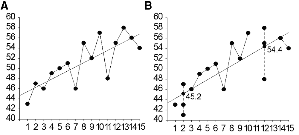
Example data set of oral reading fluency probes over 15 weeks (a) and a static performance analysis for repeated probes with aggregation of adjacent scores on Week 2 and Week 12 (b).

The first method, applied at Week 2, is termed “multiple trials” in applied regression, which translates to “multiple probes” in PM. A minimum of three (some experts permit as few as two) independent probes are administered at Week 2 (41, 43, 47), an increase over the apparent normal schedule of one per week. These scores are not averaged but are entered individually, all at Week 2. As shown in Figure 1b, the best estimate of student performance at Week 2 is neither the median of these three scores (43) nor their mean (43.67). The best estimate is instead the point on the linear regression trend line (black dot) that equals 45.2. This 45.2 value is termed an “estimated score,” a Yest or Yhat score, and is a normal output from a linear regression module. Its calculation does include all three scores from Week 2 but its precision benefits from all other scores in the series as well. By drawing on the full data set, the Yest score is a more precise estimate of static performance at a given week. It also is stable, not unduly influenced by a single score at Week 2 or any other time.

Yest scores do not need to be hand calculated; they are routinely output by most linear regression statistics programs. Data are input as X predictor = Time and Y criterion = Score. Within the regression program, the user simply specifies a time (e.g., weeks) and requests that Yest be output. Yest is sometimes confusingly referred to as “predicted Y” but is not necessarily a future prediction. This terminology is confusing because it is only CIs, not prediction intervals (PIs), that are desirable in PM.

Figure 1b at Week 12 shows the second method for estimating static performance at a given week, through “approximate repeats.” Three (some say as few as two) adjacent scores are identified, for example, for Weeks 11, 12, and 13. Then the time for each of these three data points is changed to the median value—in this example to 12 (Week 12). Neither means nor medians are calculated. The three individual data points are entered separately, but all on Week 12. The best estimate of static performance at Week 12 (black dot on the trend line) is again the “estimated score,” or Yest.

Technical notes

The best estimate of student performance from regression will always be a point on the regression line, a Yhat or Yest score. For practical decision making, guidance comes from texts in business, health, and the physical sciences (Armitage, Berry, & Matthews, 2002; Draper & Smith, 1998; Graybill & Iyer, 1998; Neter, Kutner, Nachtsheim, & Wasserman, 1996). These texts offer multiple examples of a Yest score whose SE, SE _Yest , is based on a small “group of scores” or “multiple observations” at one time, as few as two, although three is commonly recommended (Neter et al., 1996). The data may be from a single respondent, and the remaining times may contain only one data point. The multiple (minimum three) observations must be independently obtained, that is, “independent trials,” but may be from the same respondent (Neter et al., 1996). The second aggregation method of “approximate repeats” is referred to explicitly by Draper and Smith (1998, p. 42). Proximal aggregation also is used in other texts, but without being named.

2. Fitting a Level of Confidence to an Educational Decision

Few within-classroom (lower stakes) data-based decisions need to consider measurement error. This article focuses only on medium- and high-stakes decisions made from an individual student’s PM data. These decisions require that score summaries be expressed with their known measurement error. But there is a prior step—choosing a “level of confidence,” such as 80%, 85%, 90%, or 95%. Selection should be based on our willingness to accept the costs of making an error, wrong decision, or “regretted decision” (Goodman, 1999). Selection of a 95% level of confidence means willingness to accept wrong decisions at the rate of 5 per 100 (1 per 20). By contrast, selection of an 80% level of confidence means tolerance of a much higher rate of “regretted decisions”: 20 per 100 (1 per 5). Judging the social-emotional, physical, and financial costs of an error is required in a field such as medicine (Djulbegovic, Hozo, Schwartz, & McMasters, 1999; Ioannidis, 2005), but schools have little such experience. In schools, unlike in medicine, regretted decisions may be reviewed and even reversed, which argues for a less stringent level of confidence. However, the effects of a regretted decision may not be fully reversible. The stigma of labeling, special class placement, disruption of a social network, and lost opportunities to learn may not be fully reversible.

Presently, one-shot and pre–post assessments in schools commonly employ a CTT-based 95% confidence level, as recommended by test producers. Lower levels of 90% or 85% are uncommon. But as PM data are used for a range of decisions, these lower levels can serve for medium-impact, reversible decisions made every few months. The 85% level will better serve in-class decisions that are more easily reversed and may be reviewed every few months or so. The 90% level may serve decisions lasting a semester or year but that are open to review within this time and can practically be reversed. The 95% level of confidence (tolerating only 1 erroneous decision per 20) should be reserved for decisions with the highest risks: those with substantial social or educational impact, those with lasting impact, and those that are not easily reversible (American Educational Research Association, American Psychological Association, & National Council on Measurement in Education, 1999).

The problem with selecting a 95% level for low-impact, within-class decisions is that much PM data will possess too much error. Decision making is paralyzed when measurement error of an assessment exceeds the desired level of confidence. Thus, schools should choose the minimum level of confidence for a tolerable error rate. Practical data-based decision making requires a match among (a) the costs of making an error, (b) a selected level of confidence, and (c) measurement error in scores. This first of these three is a social judgment. The second and third are reflected (respectively) in (a) the selection of a confidence band or interval for a score and (b) the actual width of that band around the score.

3. Expressing a Yest Score With Its Measurement Error

Expressing a Yest score along with its CI expresses the score’s measurement error and signals to decision makers the limits on the score’s practical usefulness. Including measurement error with a Yest score is important when the score is to be used for serious decisions. The previous section focused on the early step of choosing a level of confidence well matched to the social consequences of the decision. This section demonstrates how the CI around a Yest score is expressed and interpreted.

Figure 2 depicts three confidence bands or intervals around two estimated Y (Yest) scores. Note that both Week 2 and Week 12 are represented by three data points. For Week 2 performance an 85% CI is shown, and for Week 12 both 80% and 95% intervals are shown. These three levels of confidence would be appropriate for three different types of decisions with different “costs of an erroneous decision.” The CI is defined by its upper and lower limits, which are provided in Figure 2. One can be “quite sure” (80%, 85%, or 95% sure) that the true value for the calculated Yest score is somewhere between the upper and lower CI limits.

Figure 2.

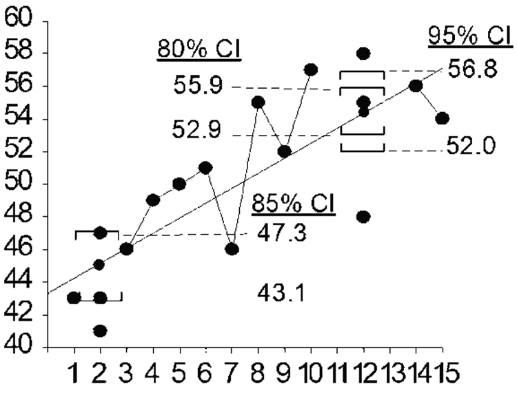
Yhat confidence intervals for three levels of confidence.

For example, it can be said about static performance at Week 12 that “we are 95% certain that the true performance level is somewhere between 52 and 56.8.” This high 95% level of confidence results in a wider CI than does the modest 80% level. With a wider CI we are less certain of where the true score lies and so less able to make needed decisions. Data may be useless for high-stakes decisions requiring a 95% confidence level but adequate for lower stakes decisions requiring an 80% confidence level, hence the need to use data with low measurement error for high-stakes decisions that require a high level (95%) of confidence.

Technical notes

Considerable confusion exists about CIs from linear regression (Schwarz, 2007). The Yhat being estimated near the center of the interval is not an individual score but rather a population mean parameter and must accordingly be based on multiple obtained scores at one time (Draper & Smith, 1998). Yet for a single client only one score typically exists at each time period, so some feel compelled to use the very unfavorable PI, which is often 2 to 3 times wider than the CI. But that use of a PI is not correct; the PI is for a “single new score,” and one not used within the calculation of the PI (Draper & Smith, 1998). For PM, error is not desired for a “single new score” but rather for the most stable estimate of student ability at a given time, which is Yest. We do caution that the ability of PM to use the CI rather than the PI does require multiple scores entered at the estimation time, hence the two methods presented earlier: multiple probes and “approximate repeats.”

The CI and the PI are both directly output from most linear regression programs, calculated from their respective SEs. The SE for the CI around a mean is $S E_{Y h a t . G} = {(M S E r r)}^{1 / 2} * {[(1 / N) + ({(X - \bar{X})}^{2} / (V A R_{x} * (N - 1))]}^{1 / 2}$ . For the PI around an individual score, it is $S E_{\Pr e d . I} = {(M S E r r)}^{1 / 2} * {[1 + (1 / N) + ({(X - \bar{X})}^{2} / (V A R_{x} * (N - 1))]}^{1 / 2}$ . The two formulas are identical except for the addition of a 1 under the radical sign of the SE for the PI. This small difference inflates the PI so much that textbooks warn against attempting to use the PI for practical decision making with most data (Armitage et al., 2002; Draper & Smith, 1998; Graybill & Iyer, 1998; Neter et al., 1996). Using an example from Figure 1b, the 80% CI for Week 12 scores was 52.9 to 55.9, 3 points wide. The 80% PI for an individual score at Week 12 is 49.8 to 59.0, which is 9.2 points wide. The PI width more than 3 times the CI width is typical.

From regression, the SE of the estimate (SE_est) is sometimes erroneously thought to be an SE for individual scores. In fact, SE_est is a misnomer (Kozak, Kozak, Staudhammer, & Watts, 2008). It is not really an SE of an estimated parameter at all (Brown, 1996). It instead expresses the dispersion of all data from the trend line, SE_est = ((SS_y * (1 − R²)) / (N − 2))^1/2, which also equals “root mean square error” or “root mean square residual,” SE_est = (MSErr)^1/2. Another misunderstanding about SE_est is that it is “scale bound”; it lacks meaning outside of a particular measurement scale, so SE_Meas should not be compared across studies unless the time and score scales match. Because it is in SD units, SE_est does have one useful interpretation. If SE_est = 11, then about 68% (±Z = 1) of the observations are expected to lie within ±11 points from the trend line.

4. Judging Reliable Improvement From One Time to a Later Time

It is often useful to compare performance levels between two points in time. This can be accomplished with PM data, and when the comparison is to serve medium- and high-stakes decisions, one should calculate “reliable improvement,” that is, considering measurement error. Reliable improvement can be calculated by a student t test but also can be judged visually from nonoverlapping CIs. As stipulated earlier, each time point should include at least three data points, permitting the use of the favorable SE for a “group of scores” in a series. Most regression programs permit the user to specify a confidence level, and for this comparison an 83.4% (83% or 84% are both commonly used) level should be selected (Schenker & Gentleman, 2001). CI overlap is defined as when the lower CI limit of the larger score drops below the upper CI limit of the smaller score. When the two 83% CIs do not overlap, then we can say with 95% certainty that the student has made “statistically significant” improvement. This overlap can be judged by glancing at CI limits of the two scores. It also can be judged by visual analysis of these CIs on a graph. Figure 3 shows the 83% CIs around Yest scores at Weeks 2 and 12.

Figure 3.

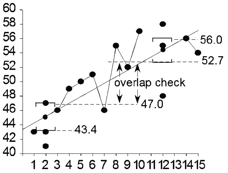
Illustration of overlap between the 83% confidence intervals of Yest scores at Weeks 2 and 12.

Their respective CIs do not overlap (52.7 is higher than 47), so we can be quite (95%) sure that the student did improve from Week 2 to Week 12.

Technical notes

Statistical testing by nonoverlapping CIs is supported by several measurement studies, including two Monte Carlo simulations (Browne, 1979; Goldstein & Healy, 1995; Payton et al., 2003; Payton, Miller, & Raun, 2000; Schenker & Gentleman, 2001). In most cases it is a good approximate method. Judging 83% CI overlap is quite accurate when the two scores being compared have similar SEs, as would any two scores from the same data series. In the unlikely occurrence of very different SEs (with a ratio of 4 or 5 to one or greater), then the nonoverlapping CI test loses power. A correction method has been provided for such cases (Payton et al., 2003). The SEs for two Yest scores from a single data series are most different when they are at different distances from the center of the time scale. For our example data, SEs for Yest at Weeks 1 and 6 or at Weeks 6 and 12 would differ the most. But for Weeks 2 and 12 the SEs for Yest are 1.21 and 1.14, respectively, a difference so small as to have no practical impact. For linear regression programs that output the SE but not upper and lower confidence boundaries or limits, this CI overlap method may offer few advantages. A standard t test will be more accurate. The major benefits of the CI overlap method are (a) results are directly output from many regression modules, with no calculations required, and (b) it can be plotted on a time series graph and is open to visual analysis.

5. Proper Uses of Slope Versus Trendedness

“Rate of improvement” or “trend line slope,” calculated as (rise/run), is the most common improvement summary from PM data. However, it has distinct limitations, and for some purposes “slope” is less desirable than an alternative, “trendedness,” summarized by R and R². Slope should not be used when “growth rates” or “improvement rates” are compared across different scales and skills, as slope is not a standardized index. Figures 4a and 4b help show the difference between slope and a standardized trendedness index (Pearson R or R²).

Figure 4.

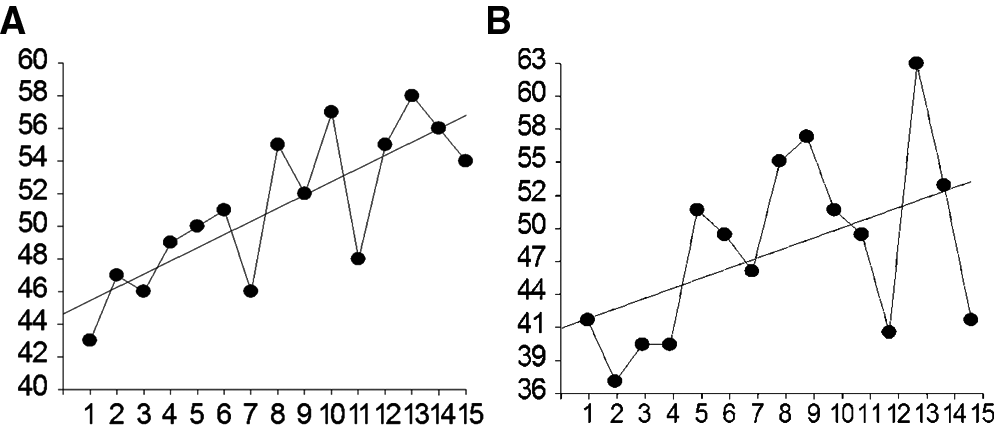
Progress monitoring data with relatively low variability (a) and much higher variability (b).

In Figure 4a, overall growth is apparent despite considerable variability or “bounce” in data toward the center of the series. A linear regression line has been fit to the Figure 4a data, from which a slope can be calculated as (rise/run). The line rises 11.34 points over the 14 weeks, so the slope is 11.34/14 = .81 points per week. The scores in Figure 4b appear quite different, with considerable more variability or “bounce,” and we would be less satisfied with the supposed improvement displayed for this student. Yet the “best fit” regression line in Figure 4b has a rise of 11.2 points over 14 weeks, so rise/run = 11.2/14 = .80, nearly the same slope as in Figure 4a. Although the slopes of Figures 4a and 4b are nearly identical, the tendency of individual scores to follow those slopes varies greatly. This tendency of individual scores to follow a trend or “trendedness” may be at least as important as slope in judging student improvement.

Trendedness is the consistency with which scores continue to move up over time, and is summarized by R and R². In Figure 1a, there is greater consistency in upward movement over time, that is, most data points are reasonably close to the line, yielding R = .79, and R² = .62. We can say that about 62% of score differences can be described as linear improvement over time. That degree of trendedness is substantial—well beyond chance levels (p = .0005). In Figure 4, data show less improvement consistency—less trendedness. More data points are far from the line, so the trendedness index, R = .48 and R² = .23. Only 23% of score differences can be described as linear improvement over time. This amount of trendedness is only borderline significant (p = .07).

Slope summaries pervade PM, but one could argue that trendedness indices R or R² are at least as useful. Do we most want to see a steep trend line or scores that improve with high consistency over time? Although steep trend and a high degree of trendedness tend to go hand in hand, they do not always. With very short data series, one commonly sees steep slopes but low trendedness or low upward consistency as measured by R and R². Both slope and trendedness reference a trend line slope summarizing its incline and R or R² its distance from the data points. A more complete summary could include both. An alternative solution, described later, is to include CIs around a slope, or at minimum a p value to indicate whether the slope is beyond chance level. Though these solutions would ameliorate one limitation of slope, they cannot fix another, which is described next.

A second limitation of slope that is overlooked is that slope is scale bound, that is, its interpretation depends on the particular score scale used. A slope’s interpretation depends on the score range, number of items, content, breadth, and difficulty level of a set of probes. By contrast, R and R² are “scale free,” so they can be used to compare progress across different sets of probes and even different skill areas. Slope’s “improvement rate” must be interpreted separately for a set of probes covering long division versus a second with a mix of short and long division items. The improvement slope for spelling accuracy with a content domain of Grade 1, 2, and 3 words is interpreted differently from the slope from probes containing only Grade 2 words. These differences in scale do not, however, affect interpretation of the standardized trendedness indices R and R².

6. Expressing “Rate of Improvement” (Slope) With Error

The common summary of dynamic improvement in PM is trend line slope. For medium- and high-stakes decisions, slope should be communicated along with its measurement error. The slope SE as well as CIs for any chosen confidence level are common outputs from a regression program. Confidence limits around a slope also can be depicted graphically. Figure 5 contains data collected over 14 weeks, with three probes administered in the first and last weeks to justify using the favorable group CIs for Yest scores.

Figure 5.

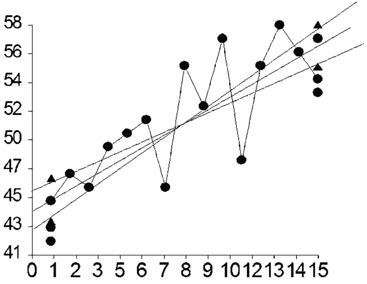
Example data set depicting confidence intervals around a slope.

The regression slope is 0.815. The two lines pivoting from its center represent upper and lower limits at the selected 83.4% confidence level. The steepest line is the upper bound, with slope = 1.0028, and the lower bound has slope = 0.63. The plotted triangles are the 83.4% CIs around Yest at Weeks 1 and 15. Close examination shows that the Yest CIs are quite close to the outer boundaries for the slope, though not exactly the same. This close similarity is always the case.

For medium- and high-stakes decisions, good slopes should be expressed with their upper and lower CI boundaries at a confidence level that is reasonable given the “costs of a regretted decision.” The CIs around a slope also allow the comparison of slopes across students (assuming they are using the same set of probes) or a student’s slope in the fall with his or her slope in the spring. The method of 83.4% CI overlap described earlier for two Yest scores also applies to comparing two slopes. The method also can be used to compare the “rate of improvement” between two students, as long as the same set of probes has been used.

7. Controlling Autocorrelation

An obstacle to analysis of PM data is serial dependence or autocorrelation (r_auto) commonly found in time series data (Sharpley & Alavosius, 1988; Suen & Ary, 1987, 1989). r_auto violates the assumption of data independence that applies to most statistical tests. r_auto is the undesirable predictability of a data point from its immediately preceding neighbor (lag-1 r_auto). A perfect linear trend line is 100% autocorrelated but is of a benign type because linear improvement is expected and desired. Undesirable r_auto in PM data is that remaining after removal of linear trend (Busk & Marascuilo, 1988; Manolov & Solanas, 2008; Matyas & Greenwood, 1996; Parker, Cryer, & Byrns, 2006). The solution to r_auto in PM data is to model it, identify it, and remove it. However, that can affect the main calculations of slope and trendedness, CIs, and p values as well as the visual configuration of data. r_auto is a nuisance, whose removal ideally causes minimum change in these other indices. Successful removal minimizes this collateral damage yet still reduces r_auto to an acceptable level.

r_auto may be positive or negative, but only positive r_auto is of great concern. Positive r_auto is visible as stretches of “persistence” in data direction; a rising data point tends to be followed by another rise and then another, or falling data similarly following one another in continuous stretches. Negative r_auto is the tendency to alternate between rising and falling data points, creating a sawtooth pattern. Negative r_auto is commonly seen in data with low reliability (Salkind, 2007). Although negative r_auto is not desirable, it does not present the obstacle to interpreting results that positive r_auto does.

The Durbin–Watson test of r_auto is a common output from linear regression, ranging from 0 to 4, with 2 signaling no r_auto and less than 2 increasing levels of positive r_auto. Values of less than 1.25 signal dangerous levels of positive r_auto (Yaffee & McGee, 2000), regardless of the p value. A second test of r_auto, the lag-1 correlation test, is also a common linear regression output. Positive lag-1 values greater than .20 or .25 signal dangerous r_auto levels, regardless of their p values (Matyas & Greenwood, 1996). For short data series, one should not rely on the p values for Durbin–Watson or lag-1 tests to determine whether dangerous r_auto exists or not.

The past 5 years have seen r_auto techniques built seamlessly into linear regression modules for time series data, requiring no extra effort by the user. Typical is the Multiple Regression with Serial Correlation module, new in the 2007 version of NCSS (Hintze, 2007). And even more useful for PM practitioners is the free 2009 version of gretl (Gnu Regression, Econometrics and Time-series Library; Cottrell & Lucchetti, 2009). Freely downloadable from http://gretl.sourceforge.net/, gretl offers a choice of three r_auto control methods within linear regression: Cochrane–Orcutt, Hildreth–Lu, and Prais–Winsten. All provide graphs of original and transformed scores, so the user can judge the amount of distortion caused by removing r_auto. Gretl provides full statistical output and can save residual, original, and transformed scores.

Figure 6 presents four published data sets with similar configurations to show the effects of r_auto cleansing. Each graph contains original scores (circles) and scores cleansed of autocorrelation (triangles). The related Table 1 reports changes in r_auto and Durbin–Watson as well as changes in slope, p values, and r from cleansing. The selection of these data sets was not random but purposeful to show typical effects.

Figure 6.

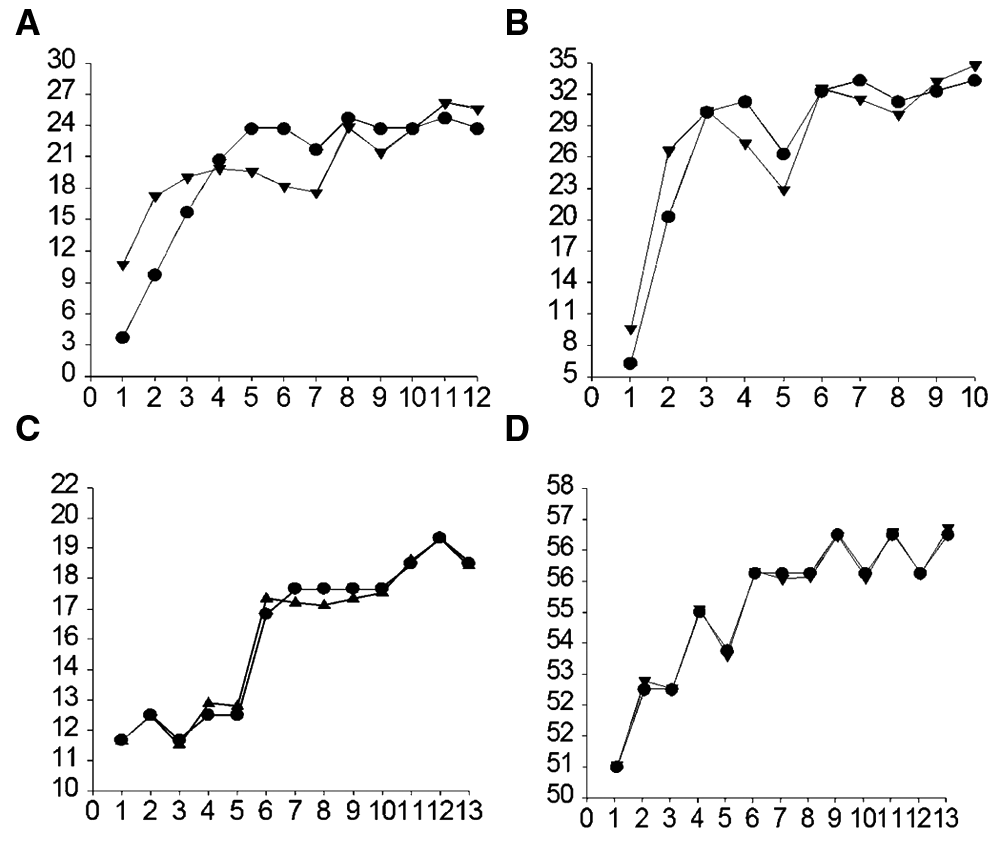
Four example data sets that show the effects of cleansing autocorrelation from typical progress monitoring data.

Table 1.

Changes in Data Values After Autocorrelation Cleansing

	Original					Cleansed of autocorrelation
Data set	r _auto	Durbin-W	Slope	p value	R	r _auto	Durbin-W	Slope	p value	R
A	.56	0.45	1.48	.001	.78	.03	1.75	1.04	.000	.87
B	.23	0.99	2.08	.014	.74	.09	1.71	1.77	.015	.73
C	.35	1.21	0.70	.000	.92	.09	1.68	0.70	.000	.93
D	.15	1.37	0.43	.002	.89	.09	1.87	0.41	.000	.87

Abbreviations: r_auto, parameter estimate of autocorrelation; Durbin-W, Durbin–Watson test of autocorrelation.

Initial r_auto levels (lag-1) ranged from .15 to .56, whereas cleansed scores were all below r_auto = .10. Durbin–Watson initial levels ranged from 0.45 to 1.37, whereas cleansed levels were all close to the Durbin–Watson neutral value of 2. Thus, control of r_auto was successful in these four typical data sets.

Control of r_auto is a technical adjustment, and changes in the appearance of PM graphs should be minimized. Graph distortion disallows visual analysis and does not permit visual and statistical analysis to work together. Visual analysis of Figure 6a shows considerable distortion, whereas for Figure 6d it is barely discernable. These results match what we see in daily analysis—that correcting only large r_auto levels of .50 or .55 and higher badly distorts the graphic display. With smaller initial r_auto levels below .45 or .40, cleansing is usually effective and distorts little. Also note in Table 1 that cleansing data tends to change R and p values very little. The slope is more volatile, showing more change, which is yet another way that R is a more dependable summary than slope.

Understanding the practical effects of r_auto on PM data is a new concern for our field, with much still unknown. A study is under way by these authors comparing three leading methods of r_auto control (all available in free gretl software): Cochrane–Orcutt, Hildreth–Lu, and Prais–Winsten. Our tentative, informal judgment at this point is that Prais–Winsten is equal or superior to the others on four criteria: (a) complete removal of r_auto, (b) minimal change in graph configuration, (c) minimal change of slope, R, and p values, and (d) maintenance of all data points rather than losing one, as most techniques do.

Technical notes

Nearly a dozen methods have been advanced in the past two decades to control autocorrelation (SAS software offers six), but we found none field tested with typical single-student PM data. The best researched method is the “autoregressive integrated moving average” (ARIMA) approach (Box & Jenkins, 1976; Glass, Willson, & Gottman, 1975). ARIMA backcasting with a lag-1 (AR-1) model showed good results in field testing with single-participant time series data (Parker, 2006). But ARIMA analysis is complex and requires a dedicated ARIMA module. By integrating r_auto control into standard linear regression in software such as gretl, for the first time casual users of regression can control r_auto.

Conclusions and Recommendations

For special educators, school psychologists, and other assessment specialists in schools, the use of PM for medium- and high-stakes decision making requires new knowledge and skills. For PM data, the reliabilities, SEs, and even CIs calculated within a CTT model are inadequate. PM is open to sources of error that do not exist in a simple retesting. The purpose of this article was to present seven practical skills for PM that are unlikely to have been learned in CTT-based training:

Estimating a static performance level in PM

Fitting a level of confidence to an educational decision

Expressing an estimated score (Yhat) with its measurement error

Judging reliable improvement from one time to a later time

Properly using slope versus trendedness

Expressing “rate of improvement” (slope) with error

Controlling autocorrelation

Together, these skills and understandings should arm special educators and others to make effective use of PM data for important school decisions. None of this information is new; it all has been available in articles and texts on fixed linear regression and N = 1 time series data but is rarely if ever applied to PM in schools.

Because of the expansion of the CTT error model beyond its range of usefulness, PM practitioners tend to make only partial use of the regression alternative. For example, calculation of a static level of performance from PM data is rarely seen, and when it occurs it is most likely simply taking the mean or median of scores collected on the same date. That approach does not make use of the full series of scores as does the regression model. And use of the CTT model to estimate the reliability of a set of probes has caused reliability to be overestimated at levels not substantiated by examination of PM data from the same probes.

Here we lend some perspective to acquiring the seven skills covered in this article. First in logical order is the consideration of confidence levels appropriate to various decisions. Confidence levels have equal importance within CTT and regression, so choosing a reasonable level based on the costs of a “regretted decision” is a general skill needed for all medium- to high-stakes measurement within both models. In this article the term medium- to high-stakes decisions was used advisedly. It will not be productive to paint all decisions as either low or high stakes. A range between these two extremes fits most decisions, for which the relatively unused confidence levels of 90% and 85% are appropriate. Those options to the reified 95% level will be needed when educators frankly assess the costs of “regretted decisions.”

The next needed skills for PM practitioners are dramatically new: selecting “estimated Y” or Yest scores based on three scores on the same date or close together in time. Educators are used to dealing with obtained scores and conceptualizing true scores, but Yest scores are new. The best “conceptual handle” on Yest scores is probably visual—all are located on the regression line. Making Yest scores visually accessible may encourage their acceptance.

Although Yest scores may sound alien, they are normal outputs from most ordinary least squares linear regression modules. Not only is the Yest provided on request, but also its CI is provided, without computation. But the user must select the CI for a small “group” of scores rather than a very wide PI for an “individual” new score. There is general misunderstanding in many fields on when a CI versus PI should be used, which this article attempted to clarify in nontechnical terms. Only the CI is recommended, and only when bolstered by three (or rarely two) repeated trials or “approximate repeats.”

The skill of judging “reliable differences” between two (Yest) scores (or between slopes) by judging nonoverlap between 83.4% (one may choose either 83% or 84%) CIs will be novel for most educators. Educators do commonly compare scores but seldom obtain “reliable differences” between the scores. Reliable differences are differences that include measurement error, a requisite for medium- to high-stakes decisions. The method of CI nonoverlap is not presented for its high precision, as it may be inferior to a t test. It is presented instead because (a) it requires only visual judgment without computation, (b) requisite CIs are common output, and (c) it should be more understandable than SE calculations. The goal is not to devise more sophisticated statistical tools but rather to make sound practices approachable by school personnel.

The many strengths of PM give it great appeal, especially for students with disabilities and those at risk for failure. Its ability to provide frequent feedback, its ability to measure gains cumulatively, and its use for goal setting commend it as a key tool for student program decisions. But its use for medium- to high-stakes decisions requires additional statistical tools and skills. They will permit consumers to judge the extent to which PM can fill this new role.

Footnotes

Declaration of Conflicting Interests

The author(s) declared no potential conflicts of interest with respect to the authorship and/or publication of this article.

Funding

The author(s) received no financial support for the research and/or authorship of this article.

References

American Educational Research Association, American Psychological Association, & National Council on Measurement in Education. (1999). Standards for educational and psychological testing. Washington, DC: Author.

Ardoin

S. P.

Christ

T. J.

(2009). Curriculum based measurement of oral reading: Estimates of standard error when monitoring progress using alternate passage sets. School Psychology Review, 38, 266–283.

Armitage

Berry

Matthews

J. N.

(2002). Statistical methods in medical research (4th ed.). Oxford, UK: Blackwell.

Bolt

(2005). Reflections on practice within the heartland problem-solving model: The perceived value of direct assessment of student needs. California School Psychologist, 10, 65–80.

Box

O. E. P.

Jenkins

G. M.

(1976). Time-series analysis: Forecasting and control (2nd ed.). San Francisco, CA: Holden-Day.

Brown

J. D.

(1996). Testing in language programs. Upper Saddle River, NJ: Prentice Hall.

Brown-Chidsey

Steege

M. W.

(2005). Response to intervention: Principles and strategies for effective practice. New York, NY: Guilford.

Browne

R. H.

(1979). On visual assessment of the significance of a mean difference. Biometrics, 35, 657–665.

Busk

P. L.

Marascuilo

L. A.

(1988). Autocorrelation in single-subject research: A counter-argument to the myth of no autocorrelation. Behavioral Assessment, 10, 229–242.

10.

Christ

T. J.

Coolong-Chaffin

(2007). Interpretations of curriculum-based measurement outcomes: Standard error and confidence intervals. School Psychology Forum, 1, 75-86.

11.

Cohen

(1983). Applied multiple regression/ correlation analysis for the behavioral sciences (2nd ed.). Hillsdale, NJ: Lawrence Erlbaum.

12.

Cohen

West

S. G.

Aiken

L. S.

(2003). Applied multiple regression/correlation analysis for the behavioral sciences (3rd ed.). Mahwah, NJ: Lawrence Erlbaum.

13.

Cottrell

Lucchetti

(2009). Gnu regression, econometrics and time-series library [Computer software]. Retrieved from http://gretl.sourceforge.net/

14.

Crocker

Algina

(1986). Introduction to classical and modern test theory. Orlando, FL: Harcourt Brace.

15.

Deno

S. L.

(1985). Curriculum-based measurement: The emerging alternative. Exceptional Children, 52, 219–232.

16.

Deno

S. L.

(2003). Developments in curriculum-based measurement. The Journal of Special Education, 37, 184–192.

17.

Deno

S. L.

Deno

Marston

(1987). Test of reading fluency: Measures for screening and progress monitoring. Minneapolis, MN: Children’s Educational Services.

18.

Deno

S. L.

Fuchs

L. S.

Marston

Shin

(2001). Using curriculum-based measurement to establish growth standards for students with learning disabilities. School Psychology Review, 30, 507–524.

19.

Djulbegovic

Hozo

Schwartz

McMasters

(1999). Acceptable regret in medical decision making. Medical Hypotheses, 53, 253–259.

20.

Draper

N. R.

Smith

(1981). Applied regression analysis (2nd ed.). New York, NY: John Wiley.

21.

Draper

N. R.

Smith

(1998). Applied regression analysis (3rd ed.). New York, NY: John Wiley.

22.

Francis

D. J.

Shaywitz

S. E.

Stuebing

K. K.

Shaywitz

B. A.

Fletcher

J. M.

Lyons

G. R.

(Ed.). (1994). The measurement of change: Assessing behavior over time and within a developmental context. In Lyons

G. R.

(Ed.), Frames of reference for the assessment of learning disabilities: New views on measurement issues (pp. 29–58). Baltimore, MD: Brookes.

23.

Fuchs

L. S.

Fuchs

(2002). Curriculum-based measurement: Describing competence, enhancing outcomes, evaluating treatment effects, and identifying treatment nonresponders. Peabody Journal of Education, 77(2), 64–84.

24.

Fuchs

L. S.

Fuchs

Hamlett

C. L.

Waltz

Germann

(1993). Formative evaluation of academic progress: How much growth can we expect? School Psychology Review, 22, 27–48.

25.

Glass

G. V.

Willson

V. L.

Gottman

J. M.

(1975). Design and analysis of time-series experiments. Boulder, CO: Associated University Press.

26.

Goldstein

Healy

M. J. R.

(1995). The graphical presentation of a collection of means. Journal of the Royal Statistical Society A, 158(1), 175–177.

27.

Good

R. H.

Simmons

D. C.

Kame’enui

E. J.

(2001). The importance and decision making utility of a continuum of fluency based indicators of foundational reading skills for third-grade high-stakes outcomes. Scientific Studies of Reading, 5, 257–288.

28.

Goodman

S. N.

(1999). Toward evidence-based medical statistics. 1: The p value fallacy. Annals of Internal Medicine, 130, 995–1004.

29.

Graybill

F. A.

Iyer

H. K.

(1998). Regression analysis: Concepts and applications. Belmont, CA: Duxbury Press.

30.

Gresham

F. M.

(2002). Responsiveness to intervention: An alternative approach to the identification of learning disabilities. In Bradley

Donaldson

Hallahan

(Eds.), Identification of learning disabilities: Research to practice (pp. 467–519). Mahwah, NJ: Lawrence Erlbaum.

31.

Hagan-Burke

Jefferson

G. L.

(2002). Using data to promote academic benefit for included students with mild disabilities. Preventing School Failure, 46, 112–118.

32.

Hintze

(2007). Number cruncher statistical systems [Computer software]. Kaysville, UT: NCSS.

33.

Hintze

J. M.

Christ

T. J.

(2004). An examination of variability as a function of passage variance in CBM progress monitoring. School Psychology Review, 33, 204–217.

34.

Holdnack

J. A.

Weiss

L. G.

(2006). IDEA 2004: Anticipated implications for clinical practice—Integrating assessment and intervention. Psychology in the Schools, 43, 871–892.

35.

Hosp

M. K.

Hosp

J. L.

Howell

K. W.

(2007). The ABCs of CBM: A practical guide to curriculum-based measurement. New York, NY: Guilford.

36.

Ioannidis

J. P. A.

(2005). Why most published research findings are false. PLoS Medicine, 2(8), e124. doi:10.1371/journal.pmed.0020124

37.

Kavale

K. A.

Forness

S. R.

(2000). History, rhetoric, and reality: Analysis of the inclusion debate. Remedial and Special Education, 21, 279–296.

38.

Kozak

R. A.

Staudhammer

C. L.

Watts

S. B.

(2008). Introductory probability and statistics: Applications for forestry and natural resources. New York, NY: CABI.

39.

Kutner

M. H.

Nachtsheim

C. J.

Neter

(2004). Applied linear regression models (4th ed.). New York, NY: McGraw-Hill.

40.

MacMillan

D. L.

Semmel

M. I.

Gerber

M. M.

(1996). The social context: Then and now. In Kauffman

J. M.

Hallahan

D. P.

(Eds.), The illusion of full inclusion: A comprehensive critique of a current special education bandwagon (pp. 19–38). Austin, TX: Pro-Ed.

41.

Manolov

Solanas

(2008). Comparing N = 1 effect size indices in presence of autocorrelation. Behavior Modification, 32, 860–875.

42.

Matyas

T. A.

Greenwood

K. M.

(1996). Serial dependency in single-case time series. In Franklin

R. D.

Allison

D. B.

Gorman

B. S.

(Eds.), Design and analysis of single-case research (pp. 215–243). Mahwah, NJ: Lawrence Erlbaum.

43.

McGlinchey

M. T.

Hixson

M. D.

(2004). Using curriculum-based measurement to predict performance on state assessments in reading. School Psychology Review, 33, 193–203.

44.

Neter

Kutner

M. H.

Nachtsheim

C. J.

Wasserman

(1996). Applied linear statistical models (4th ed.). New York, NY: McGraw-Hill.

45.

Neter

Wasserman

Kutner

M. H.

(1983). Applied linear regression models. Homewood, IL: Irwin.

46.

Parker

R. I.

(2006). Increased reliability for single case research results: Is the bootstrap the answer? Behavior Therapy, 37, 326–338.

47.

Parker

R. I.

Cryer

Byrns

(2006). Controlling trend in single case research. School Psychology Quarterly, 21, 418–440.

48.

Payton

M. E.

Greenstone

M. H.

Schenker

(2003). Overlapping confidence intervals or standard error intervals: What do they mean in terms of statistical significance? Journal of Insect Science, 3(34), 1–6.

49.

Payton

M. E.

Miller

A. E.

Raun

W. R.

(2000). Testing statistical hypotheses using standard error bars and confidence intervals. Communications in Soil Science and Plant Analysis, 31, 547–552.

50.

Pedhazur

E. J.

(1982). Multiple regression in behavioral research: Explanation and prediction. Fort Worth, TX: Holt, Rinehart & Winston.

51.

Poncy

B. C.

Skinner

C. H.

Axtell

P. K.

(2005). An investigation of the reliability and standard error of measurement of words read correctly per minute using curriculum based measurement. Journal of Psychoeducational Assessment, 23, 226–238.

52.

Restori

A. F.

Gresham

F. M.

Cook

C. R.

(2008). Old habits die hard: Past and current issues pertaining to response-to-intervention. California School Psychologist, 13, 67–79.

53.

Salkind

N. J.

(Ed.). (2007). The encyclopedia of measurement and statistics (Vol. 1). Thousand Oaks, CA: Sage.

54.

Schenker

Gentleman

J. F.

(2001). On judging the significance of differences by examining overlap between confidence intervals. American Statistician, 55, 182–186.

55.

Schwarz

C. J.

(2007). Sampling, regression, experimental design and analysis for environmental scientists, biologists and resource managers. Burnaby, Canada: Simon Fraser University. Retrieved from http://www.stat.sfu.ca/~cschwarz/Stat-650/Notes/PDF/Chapter17.pdf

56.

Sharpley

C. F.

Alavosius

M. P.

(1988). Autocorrelation in behavioral data: An alternative perspective. Behavioral Assessment, 10, 243–251.

57.

Sheskin

D. J.

(2007). Handbook of parametric and nonparametric statistical procedures. Boca Raton, FL: Chapman & Hall.

58.

Stage

S. A.

Jacobsen

M. D.

(2001). Predicting student success on a state-mandated performance-based assessment using oral reading fluency. School Psychology Review, 30, 407–419.

59.

Suen

H. K.

Ary

(1987). Autocorrelation in applied behavior analysis: Myth or reality? Behavioral Assessment, 9, 125–130.

60.

Suen

H. K.

Ary

(1989). Analyzing quantitative behavioral observation data. Hillsdale, NJ: Lawrence Erlbaum.

61.

Will

(1986). Educating students with learning problems: A shared responsibility. Exceptional Children, 52, 411–415.

62.

Yaffee

R. A.

McGee

(2000). An introduction to time series analysis and forecasting: With applications of SAS and SPSS. San Diego, CA: Academic Press.