Testing for normality: a user’s (cautionary) guide

The assumption of normality

Statistical inference is contingent on underlying assumptions about populations. These assumptions help hypothesise the distribution of the test statistic under the null hypothesis (H₀) and consequently derive p-values from empirical data. The confirmation of these assumptions in animal research plays a vital role in preserving research quality and preventing the unnecessary use of animals, thus warranting its inclusion in the ARRIVE guidelines (item 7.b). ¹ One such assumption is the assumption of normality, which matters particularly for parametric tests. For example, in linear regression, the constraint of normality concerns the sampling distribution of slope estimates under H₀, which is authorized by normality of population errors (i.e., the remaining distances between observations and their estimates). However, normality cannot be presupposed agnostically because natural variables are often non-normal,^2–5 and the support of the assumption must arise from interrogating the data. In the regression example above, the conjecture of the normality of population errors is therefore based on the analysis of data residuals. The present review provides a summary of common methods that probe data conformity with normality, putting emphasis predominantly on their interpretation and limitations. For a more thorough mathematical discussion, the reader may consult excellent reviews. ⁶ The literature presents the assumption of normality from various perspectives, which can be perceived as confusing. In this essay, the decision is made to offer a narrative based on errors and residuals, because statistical tests often boil down to regression analysis.

Qualitative visual examination

Diagrammatical displays provide very accessible methods to examine the distribution of observations (raw data or residuals). The most popular is the histogram, which shows the frequency distribution based on binning the observations in chosen intervals. However, binning poses problems since the readability of the histogram depends on the bin widths, and discrete histograms may be difficult to compare with continuous distributions such as the normal distribution. In addition, when few observations are included, histograms tend to appear fragmented and difficult to interpret.

Quantile–quantile (QQ)-plots are another type of diagram that consists of scatter plots that compare the quantiles of the given residuals with those theoretically sampled from a normal distribution. ⁷ If the residuals were drawn from a normal population of errors, alignment of the dots would be expected on the straight bisector line. Conversely, non-alignment delivers useful information about outliers, skewness or limits of detection (Figure 1, insets). The elegance of QQ-plots comes from their easy construction, the quick visual grasp they provide of the distribution (e.g., skewed distributions such as lognormal distribution yielding curved QQ-plots) and the relative richness of the returned information. However, interpreting QQ-plots may require some practice, especially because there is a frequent and often irrelevant deviation from the line at the extremes that becomes more pronounced in cases of non-normality and because alignments may be harder to pinpoint with small samples. Finally, QQ-plots do not provide a numerical output to guide dichotomic decisions; they are also somewhat subjective and may suffer of a relative lack of consistency.

OPEN IN VIEWER

Figure 1.

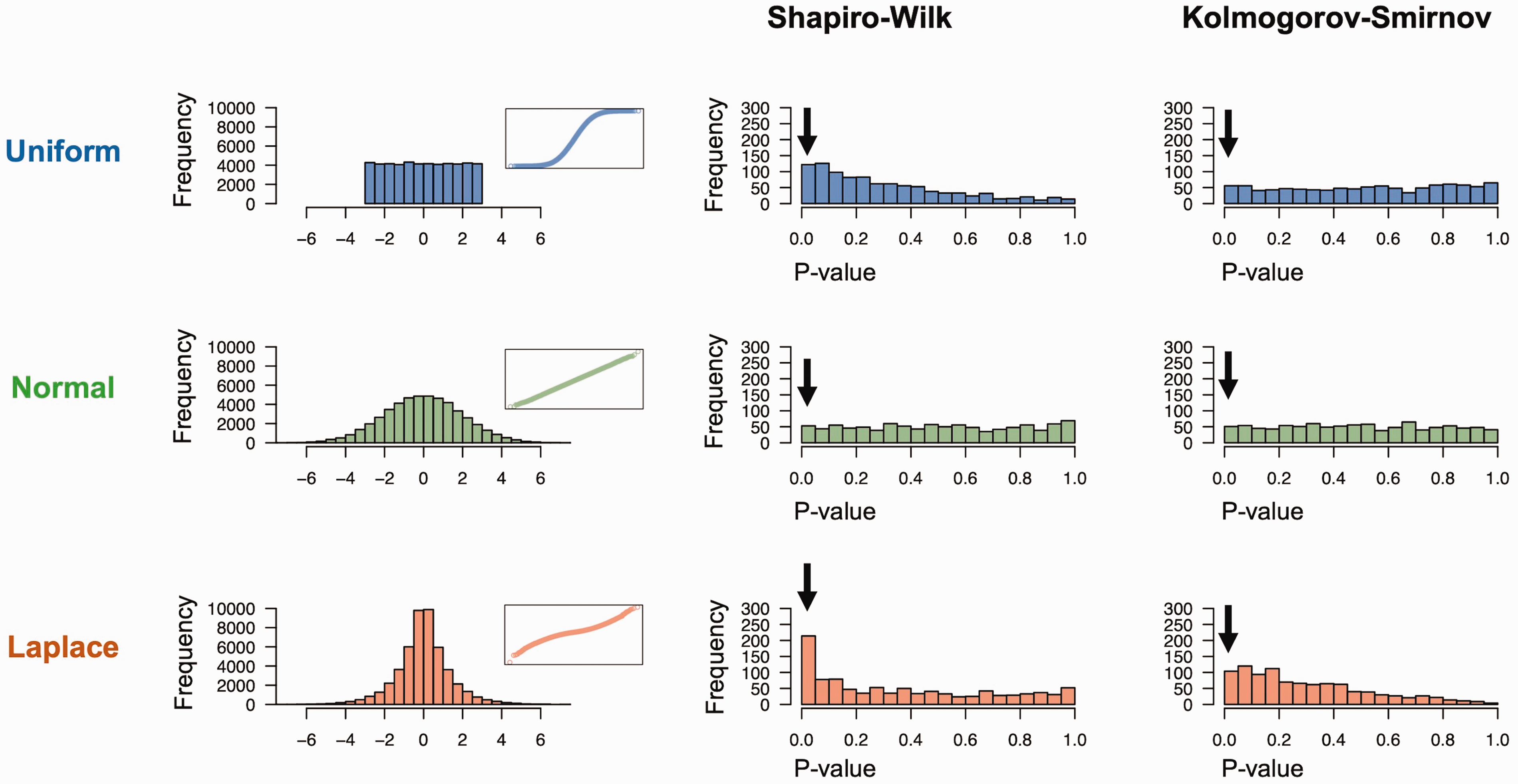
Goodness-of-fit tests have different statistical power and generate inconstant p-values. Distribution of empirical p-values (second and third columns) obtained via Monte Carlo simulations (1000 samples, n = 15 each) under H₀ of normality (mean = 0 and SD = 2), when using Shapiro–Wilk (second column) or Kolmogorov–Smirnov (third column) tests on samples from initial uniform (blue, minimum = –3, maximum = 3), normal (green, mean = 0, SD = 2) or Laplace (orange, location = 0, scale = 1) distributions. The histograms in the first column show the original distributions (n = 50,000), inserts show the corresponding QQ-plots. In the presence of genuine non-normality, p-values from the Shapiro–Wilk test display a more pronounced right skew, i.e., smaller p-values, compared with the Kolmogorov–Smirnov test, including more statistically significant p-values at the conventional 0.05 level (arrows). However, most trials return p-values above 0.05. When H₀ is true (green histograms), both tests return flat p-value distribution, corresponding to an equiprobability of all p-values.

Ad hoc goodness-of-fit tests: the snares of inference

Quantitatively, it is possible to use goodness-of-fit statistical hypothesis tests to challenge the normality assumption. These tests may be grounded on the analysis of skewness and kurtosis (e.g., D’Agostino and Pearson tests), ⁸ on the comparison of empirical and theoretical density functions (e.g., Kolmogorov–Smirnov test), ⁹ or on the covariance of the ranked residuals against the hypothetical normally transformed ones (e.g., Shapiro–Wilk test, Shapiro–Francia test).^10,11 All use an H₀ of sampling from a given distribution, some being designed explicitly for normality. They have different intrinsic statistical power, the Shapiro–Wilk and Shapiro–Francia tests having consistently shown the best performances at detecting genuine non-normality.^12–14 Employing goodness-of-fit tests requires a correct understanding of hypothesis testing where statistical significance reveals exceptionality of the observed (or more extreme) divergence from normality under H₀. Conversely, even if the population errors are non-normal, small samples will make most experiments wrongly fail to reject H₀. Just like in any hypothesis test, p-values do not embody the probability of H₀ but instead can be very inconstant, especially when samples are small. Figure 1 illustrates that, at a sample size of n = 15, although the Shapiro–Wilk test outperforms the Kolmogorov–Smirnov test in detecting true non-normality, (not surprisingly since the Kolmogorov–Smirnov test is non-parametric ¹⁵ ), the trials producing statistically significant p-values always constitute a minuscule fraction of tests. The problem with analytically testing for normality is not statistical: normality is often implicitly assumed to be true when tests do not provide enough evidence to reject normality. This idea that ‘the variable is normal, unless demonstrated non-normal’ is a logical fallacy that constitutes an archetypal instance of reversal of the burden of proof that results partly from the looked-for hypothesis of normality. One should always avoid narratives that claim ‘proofs’ of normality with goodness-of-fit tests, especially with small samples.

Is preliminary normality testing that self-evident?

Up to this point, the current text adheres to the customary practice of treating the sample-based substantiation of population normality as an obvious and essential prerequisite for parametric inference. However, voices exposing a more nuanced position have been heard recurrently. ¹⁶ Firstly, assumptions relate to the population (errors) rather than the samples (residuals), emphasizing the critical importance of the representativeness of those samples, which may be jeopardised in small samples. Secondly, since actual normality is unrealistic, goodness-of-fit tests will virtually always reject it as samples enlarge, even for microscopic mismatches. Yet, intuitively, infinitesimal divergences should not dismiss the subsequent use of parametric tests. Here, it is worth elaborating on the frequently seen recommendation to increase sample size and invoke the central limit theorem, which yields parameter estimates that are asymptotically normal even if errors are not. This approach is thought to eliminate the need for normality testing. However, it is important to note that this manoeuvre should not overshadow that the distribution of parameter estimates is just one aspect of the potential importance of normality. More precisely, normality of errors also ensures the independence of estimated mean and variance, which is a prerequisite for inference based on a t-statistic. Therefore, as previously discussed, testing for normality might be subject to debate, but arguments opposing it should not rely merely on the central limit theorem. Ultimately, whether it is necessary to test for normality revolves around the actual importance of the normality assumption itself. Parametric tests hinge upon several other assumptions, including the independence of errors and equality of variances, which are often deemed even more critical for inference. The evaluation of normality and its potential assessment would be irrelevant if these other assumptions are not met in the first place.

Conclusion and recommendations: test, not test, how to test?

I suggest combining qualitative and quantitative methods, ¹⁷ and encourage the systematic use of both a QQ-plot that will help isolate the component of potential non-normality together with a powerful analytical procedure (e.g., Shapiro–Wilk test, Shapiro–Francia test). In all cases, the inflexible planning of a statistically powerful parametric test to maximize power on small samples should never be the motivation behind inspecting normality. Rather, the potential initial assessment of normality should take place upstream of the choice of the ensuing statistical approach. Importantly, this final choice can also be driven by the investigator’s prior knowledge about the population structure. Sample size is central, and all procedures presented herein totter with small samples. Yet, I am no stranger to the fact that, in life science, small samples are often compelled by practical reasons. In that case, the data residuals should not be deemed suitable for normality testing, and one may consider using non-parametric methods. Yet, although non-parametric tests largely relax distributional assumptions, they are not an all-purpose magical cure for all designs. Indeed, non-parametric tests still require compliance with key assumptions such as independence, sampling from distributions with similar shapes (e.g., Mann–Whitney test, Kruskal–Wallis test) or exchangeability of observations (e.g., permutation test). If normality has been tested and cannot be assumed, there exist a range of possible options, which have been described comprehensively by others. ¹⁸ Finally, in line with previously published guidelines,^19,20 I suggest seeking advice from a statistician whenever in doubt.